| Issue |
A&A
Volume 580, August 2015
|
|
|---|---|---|
| Article Number | A39 | |
| Number of page(s) | 11 | |
| Section | Stellar structure and evolution | |
| DOI | https://doi.org/10.1051/0004-6361/201526318 | |
| Published online | 24 July 2015 | |
Diagnostic of stellar magnetic fields with cumulative circular polarisation profiles
Department of Physics and Astronomy, Uppsala University, Box 516, 75120 Uppsala, Sweden
e-mail: This email address is being protected from spambots. You need JavaScript enabled to view it.
Received: 15 April 2015
Accepted: 22 May 2015
Abstract
Information about stellar magnetic field topologies is obtained primarily from high-resolution circular polarisation (Stokes V) observations. Because of their generally complex morphologies, the stellar Stokes V profiles are usually interpreted with elaborate inversion techniques such as Zeeman Doppler imaging (ZDI). Here we further develop a new method for interpreting circular polarisation signatures in spectral lines using cumulative Stokes V profiles (anti-derivative of Stokes V). This method is complimentary to ZDI and can be applied to validate the inversion results or when the available observational data are insufficient for an inversion. Based on the rigorous treatment of polarised line formation in the weak-field regime, we show that, for rapidly rotating stars, the cumulative Stokes V profiles contain information about the spatially resolved longitudinal magnetic field density. Rotational modulation of these profiles can be employed for a simple, qualitative characterisation of the stellar magnetic field topologies. We apply this diagnostic method to the archival observations of the weak-line T Tauri star V410 Tau and Bp He-strong star HD 37776. We show that the magnetic field in V410 Tau is dominated by an azimuthal component, in agreement with the ZDI map that we recover from the same data set. For HD 37776 the cumulative Stokes V profile variation indicates the presence of multiple regions of positive and negative field polarity. This behaviour agrees with the ZDI results, but contradicts the popular hypothesis that the magnetic field of this star is dominated by an axisymmetric quadrupolar component.
Key words: magnetic fields / stars: activity / stars: magnetic field / stars: individual: V410 Tau / stars: individual: HD 37776
© ESO, 2015
1. Introduction
Stellar magnetism represents an important ingredient of the theories of stellar formation and evolution, if not fully understood and poorly constrained as yet. Although magnetic fields are believed to play an important role in many astrophysical situations, their direct detection and characterisation is often very challenging. The stellar surface magnetic fields with typical strengths ranging from a few Gauss to several kilo-Gauss are commonly diagnosed with the help of the Zeeman effect. The broadening and splitting of magnetically sensitive spectral lines becomes apparent in high-resolution spectra when the field strength exceeds ~1 kG, allowing one to measure the mean field modulus (Mathys et al. 1997; Kochukhov et al. 2006; Reiners & Basri 2007) and identify different field components (Johns-Krull & Valenti 1996; Shulyak et al. 2014) in strongly magnetised objects. However, this Zeeman broadening analysis is limited to slow rotators and provides little information about the magnetic field geometry. On the other hand, analysis of circular (and more recently linear) polarisation in spectral lines enables detection of much weaker magnetic fields (Wade et al. 2000; Petit et al. 2011; Marsden et al. 2014), especially when polarisation signals can be enhanced with line-addition methods (Donati et al. 1997; Kochukhov et al. 2010). Reconstruction of the detailed surface magnetic field vector maps with the Zeeman Doppler imaging (ZDI) technique heavily relies on the interpretation of polarisation in spectral line profiles (Brown et al. 1991; Piskunov & Kochukhov 2002; Carroll et al. 2012).
For early-type magnetic stars, which typically host strong, globally organised, dipolar-like fossil fields, morphologically simple circular polarisation (Stokes V) signatures are frequently observed, with two lobes or an S-shape, for instance. Several integral magnetic observables, for example the mean longitudinal magnetic field (Mathys 1991) and crossover (Mathys 1995), can be derived by computing the wavelength moments of such simple Stokes V profiles. These observables are interpreted by fitting their rotational phase curves with low-order multipolar field models (Landstreet & Mathys 2000; Bagnulo et al. 2002). Although this technique misses some small-scale surface magnetic field structures (Kochukhov et al. 2004; Kochukhov & Wade 2010), it is straightforward to apply and computationally inexpensive and is therefore widely used to obtain information on the global magnetic field geometries of large stellar samples (e.g. Aurière et al. 2007; Hubrig et al. 2007).
In contrast to stable and usually topologically simple magnetic fields of early-type stars, the dynamo-degenerated surface fields of active late-type stars are weak, complex, and rapidly evolving. Their circular polarisation profile shapes are correspondingly more complex and often exhibit many lobes. Such Stokes V profiles cannot be meaningfully characterised with integral magnetic observables because their low-order moments tend to be close to zero even when strong polarisation signatures are evident in the data (e.g. Kochukhov et al. 2013). In other words, the surface magnetic field distribution is so complex that vector averaging over the visible stellar disk leads to a substantial cancellation of the Stokes V signal corresponding to different field polarities. In this situation, an elaborate ZDI modelling of the Stokes V profiles themselves is usually the solution, which imposes stringent requirements on the signal-to-noise ratio and rotational phase coverage of the observational data. Being an intrinsically ill-posed inversion problem, reconstruction of the stellar magnetic field topologies with ZDI suffers from a number of uniqueness and reliability issues (Donati & Brown 1997; Kochukhov & Piskunov 2002; Rosén & Kochukhov 2012), not least related to the fact that only circular polarisation and not the full Stokes vector spectra are typically available for active late-type stars. In this respect, ZDI is often perceived to be less reliable than the usual mapping of temperature spots or chemical inhomogeneities using intensity spectra. As a result of a complex response of the circular polarisation spectra to the strength and orientation of the local magnetic field, no straightforward connection between the polarisation profile variability pattern and major surface magnetic features can be established in the same way as, for example, individual star spots in the dynamic intensity spectra are recognised (e.g. Barnes et al. 2000). It is therefore of great interest to devise simple yet informative alternative methods for analysing complex Stokes V profiles that can be used to validate ZDI results or applied when the rotational phase coverage is insufficient for a magnetic inversion.
Several recent studies proposed new methods for extracting information from the circular polarisation signatures. Carroll & Strassmeier (2014) considered the diagnostic potential of the net absolute Stokes V signal, showing that under certain assumptions it allows characterising the apparent absolute longitudinal magnetic field. On the other hand, Gayley & Owocki (2015) suggested using an anti-derivative of the Stokes V profile for a more intuitive interpretation of the circular polarisation data. In this paper we develop this idea in more detail. The main goal of this work is to present a comprehensive theoretical formulation of the new polarisation observable, demonstrate its connection to the underlying stellar surface magnetic field structure, and to apply the new magnetic field diagnostic method both to simulated circular polarisation data and to real spectropolarimetric observations of stars with topologically complex magnetic fields.
2. Cumulative Stokes V profiles
2.1. Theoretical basis
To describe the disk-integrated Stokes parameter profiles of a rotating star, we consider a coordinate system with the z-axis directed towards the observer and the y-axis located in the plane formed by the line of sight and the stellar rotational axis. The star is assumed to have a unit radius and to rotate counterclockwise as seen from the visible rotational pole. Then, the Doppler shift across the stellar disk is a function of the x-coordinate alone. With these conventions the disk-integrated continuum intensity is 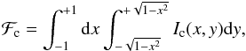 (1)and the disk-integrated Stokes profiles of a spectral line with the central wavelength λ0 are represented by the integrals
 ![Mathematical equation: \begin{eqnarray} {\cal F}_I = \int_{-1}^{+1} {\rm d}x \int_{-\sqrt{1-x^2}}^{+\sqrt{1-x^2}} I[x,y;\lambda-\lambda_0-\Delta\lambda_R x; \boldsymbol{B}(x,y)] {\rm d}y \end{eqnarray}](/articles/aa/full_html/2015/08/aa26318-15/aa26318-15-eq8.png) (2)and
(2)and ![Mathematical equation: \begin{eqnarray} {\cal F}_V = \int_{-1}^{+1} {\rm d}x \int_{-\sqrt{1-x^2}}^{+\sqrt{1-x^2}} V[x,y;\lambda-\lambda_0-\Delta\lambda_R x; \boldsymbol{B}(x,y)] {\rm d}y, \end{eqnarray}](/articles/aa/full_html/2015/08/aa26318-15/aa26318-15-eq9.png) (3)where Ic(x,y) represents the local continuum intensity, and the local line intensity and polarisation are given by I(x,y,λ,B) and V(x,y,λ,B). The amplitude of the Doppler shift that is due to the stellar rotation is determined by the projected rotational velocity vesini
(3)where Ic(x,y) represents the local continuum intensity, and the local line intensity and polarisation are given by I(x,y,λ,B) and V(x,y,λ,B). The amplitude of the Doppler shift that is due to the stellar rotation is determined by the projected rotational velocity vesini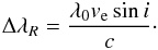 (4)Under the weak-field approximation (e.g. Landi Degl’Innocenti & Landolfi 2004), the local intensity profile is unaffected by the magnetic field, while the Stokes V profile is determined by the product of the first derivative of Stokes I and the line-of-sight component Bz(x,y) of the local magnetic field vector
 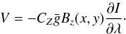 (5)In this expression
  denotes the effective Landé factor of a spectral line and
 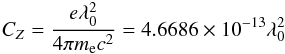 (6)for the field measured in G and wavelength in Å.
Using this approximation of the local Stokes V profile, the disk-integrated circular polarisation spectrum can be expressed as ![Mathematical equation: \begin{eqnarray} \begin{split} {\cal F}_V & =& -C_Z \bar{g} \displaystyle\int_{-1}^{+1} {\rm d}x \int_{-\sqrt{1-x^2}}^{+\sqrt{1-x^2}} B_z(x,y) \\ && \times \dfrac{\partial }{\partial \lambda} I[x,y;\lambda-\lambda_0-\Delta\lambda_R x] {\rm d}y. \end{split} \end{eqnarray}](/articles/aa/full_html/2015/08/aa26318-15/aa26318-15-eq20.png) (7)Recalling that the observed Stokes parameter profiles are normalised by the disk-integrated continuum intensity, we define the normalised disk-integrated spectral line intensity
(7)Recalling that the observed Stokes parameter profiles are normalised by the disk-integrated continuum intensity, we define the normalised disk-integrated spectral line intensity ![Mathematical equation: \begin{eqnarray} {\cal R}_I\equiv\dfrac{{\cal F}_I}{{\cal F}_{\rm c}} = \dfrac{\displaystyle \int_{-1}^{+1} {\rm d}x \int_{-\sqrt{1-x^2}}^{+\sqrt{1-x^2}} I[x,y;\lambda-\lambda_0-\Delta\lambda_R x] {\rm d}y} {\displaystyle \int_{-1}^{+1} {\rm d}x \int_{-\sqrt{1-x^2}}^{+\sqrt{1-x^2}} I_{\rm c}(x,y) {\rm d}y} \end{eqnarray}](/articles/aa/full_html/2015/08/aa26318-15/aa26318-15-eq21.png) (8)and circular polarisation
(8)and circular polarisation ![Mathematical equation: \begin{eqnarray} \begin{split} {\cal R}_V\equiv & \dfrac{{\cal F}_V}{{\cal F}_{\rm c}} = -\dfrac{C_Z \bar{g}}{\displaystyle \int_{-1}^{+1} {\rm d}x \int_{-\sqrt{1-x^2}}^{+\sqrt{1-x^2}} I_{\rm c}(x,y) {\rm d}y} \\ & \times \displaystyle \int_{-1}^{+1} {\rm d}x \int_{-\sqrt{1-x^2}}^{+\sqrt{1-x^2}} B_z(x,y) \dfrac{\partial }{\partial \lambda} I[x,y;\lambda-\lambda_0-\Delta\lambda_R x] {\rm d}y. \\ \end{split} \end{eqnarray}](/articles/aa/full_html/2015/08/aa26318-15/aa26318-15-eq22.png) (9)The latter equation can be equivalently written as
(9)The latter equation can be equivalently written as ![Mathematical equation: \begin{eqnarray} {\cal R}_V &= & \dfrac{\partial }{\partial \lambda} \Bigg\{ \dfrac{ C_Z \bar{g}}{{\cal F}_{\rm c}} \int_{-1}^{+1} {\rm d}x \int_{-\sqrt{1-x^2}}^{+\sqrt{1-x^2}} B_z(x,y) \nonumber\\ && \times \left (I_{\rm c}(x,y) - I[x,y;\lambda-\lambda_0-\Delta\lambda_R x] \right) {\rm d}y \Bigg\} \end{eqnarray}](/articles/aa/full_html/2015/08/aa26318-15/aa26318-15-eq23.png) (10)or
(10)or ![Mathematical equation: \begin{eqnarray} \begin{split} {\cal R}_V = & \dfrac{\partial }{\partial \lambda} \Bigg\{ C_Z \bar{g} \int_{-1}^{+1} {\rm d}x \int_{-\sqrt{1-x^2}}^{+\sqrt{1-x^2}} B_z(x,y) \\ & \times i_{\rm c}(x,y) r_I[x,y;\lambda-\lambda_0-\Delta\lambda_R x] {\rm d}y \Bigg\}, \end{split} \label{eq11} \end{eqnarray}](/articles/aa/full_html/2015/08/aa26318-15/aa26318-15-eq24.png) (11)where ic denotes the local normalised continuum intensity
(11)where ic denotes the local normalised continuum intensity  (12)and rI corresponds to the local normalised residual Stokes I profile
 ![Mathematical equation: \begin{eqnarray} r_I [x,y;\lambda-\lambda_0-\Delta\lambda_R x] \equiv \dfrac{I_{\rm c}(x,y) - I[x,y;\lambda-\lambda_0-\Delta\lambda_R x]}{I_{\rm c}(x,y)}\cdot \end{eqnarray}](/articles/aa/full_html/2015/08/aa26318-15/aa26318-15-eq28.png) (13)We define the cumulative Stokes V (CSV) profile as
(13)We define the cumulative Stokes V (CSV) profile as  (14)where
  (15)is the equivalent width of the disk-integrated Stokes I profile and the integration limits λmin, λmax cover the full extent of a spectral line. Substituting Eq. (11) into Eq. (14) yields
 ![Mathematical equation: \begin{eqnarray} {\cal G}_V (\lambda) &= & \dfrac{ C_Z \bar{g} }{W_I} \int_{-1}^{+1} {\rm d}x \int_{-\sqrt{1-x^2}}^{+\sqrt{1-x^2}} B_z(x,y) \nonumber\\ & & \,\,\times \,\,i_{\rm c}(x,y) r_I[x,y;\lambda-\lambda_0-\Delta\lambda_R x] {\rm d}y. \end{eqnarray}](/articles/aa/full_html/2015/08/aa26318-15/aa26318-15-eq33.png) (16)Dividing this quantity by
(16)Dividing this quantity by  provides the longitudinal magnetic field density
 ![Mathematical equation: \begin{eqnarray} \begin{split} \overline{B}_z(\lambda) \equiv \dfrac{{\cal G}_V (\lambda)}{C_Z \bar{g}} = & \dfrac{1}{W_I} \int_{-1}^{+1} {\rm d}x \int_{-\sqrt{1-x^2}}^{+\sqrt{1-x^2}} B_z(x,y) \\ & \times i_{\rm c}(x,y) r_I[x,y;\lambda-\lambda_0-\Delta\lambda_R x] {\rm d}y. \end{split} \label{eq17} \end{eqnarray}](/articles/aa/full_html/2015/08/aa26318-15/aa26318-15-eq35.png) (17)This quantity represents a velocity-resolved measure of the line-of-sight magnetic field component, weighted by the projected surface area and by the equivalent width-normalised local Stokes I profile.
(17)This quantity represents a velocity-resolved measure of the line-of-sight magnetic field component, weighted by the projected surface area and by the equivalent width-normalised local Stokes I profile.  has the units of magnetic field divided by wavelength. Its integration over the full line profile gives the normalised first moment of Stokes V
 (18)commonly known as the mean longitudinal magnetic field.
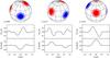 |
Fig. 1 Model Stokes V (upper curves) and cumulative Stokes V (lower curves) profiles for a star with several large circular magnetic spots of different polarities. The line profiles and the spherical maps of the radial magnetic field component are shown for three different rotational phases. The phases are indicated above each line profile panel. |
The  observable discussed above is identical to the Stokes V anti-derivative concept introduced by Gayley & Owocki (2015) with the exception that we formulate this quantity with respect to the normalised Stokes V parameter ℛV and divide the resulting profiles by WI, whereas the earlier study proposed to divide by 1−ℛI. The quantity
  discussed by Gayley & Owocki (2015) is easily recovered from our CSV profiles using the transformation
 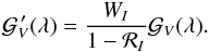 (19)The corresponding velocity-resolved mean longitudinal magnetic field
  , which can be obtained by dividing by , has the units of magnetic field strength.
The longitudinal magnetic field density or the velocity-resolved longitudinal field derived from the CSV profiles represent morphologically simpler observables than the Stokes V profiles themselves. They characterise the line-of-sight magnetic field averaged along the stripes of constant Doppler shift, thus providing a more intuitive representation of the information content of the Stokes V spectra.
Although the observables and are closely related, different normalisation choices lead to a somewhat different behaviour. The velocity-resolved mean longitudinal field closely tracks the actual local line-of-sight magnetic field component. The longitudinal field density includes an additional weighting by the projected surface area and therefore gradually diminishes to zero towards the line profile edges even if the underlying Bz distribution is uniform. The quantity compensates for the changing projected area by the 1−ℛI normalisation, but instead suffers from major noise artefacts at profile edges that are due to the division of two small numbers. Compared to , this quantity may also be adversely affected by the distortions of Stokes I profile shape caused by stellar surface inhomogeneities.
Equation (17) can be considered as a convolution integral with a kernel given by the residual Stokes I profile. The higher the ratio of ΔλR to the local profile width Δλl, the less susceptible is to the cancellation of polarisation signatures corresponding to different field polarities. Therefore, the new magnetic observable will be most effective for rapid rotators since in this case ΔλR ≫ Δλl.
Based on these definitions, we carried out an illustrative calculation of the profiles for a magnetic field distribution comprising several circular spots with the radial field strength of 0.5–1.0 kG (see Fig. 1). The calculations assumed a Gaussian shape with a FWHM = 8 km s-1 for the local Stokes I profile. The adopted central wavelength and effective Landé factor, λ0 = 5630 Å and  , corresponded to the mean values of the LSD line mask used for V410 Tau (see Sect. 3). The star was assumed to rotate with vesini = 50 km s-1 and to be inclined by i = 60° with respect to the line of sight.
Figure 1 shows the spherical maps of the radial magnetic field as well as the Stokes V and CSV profile for three different rotational phases. When the surface magnetic field distribution is dominated by one of the magnetic polarities, the Stokes V profile exhibits the classical S-shape pattern. The corresponding CSV profiles show a single bump, which can be either positive or negative, depending on the dominant magnetic field polarity. On the other hand, when several regions of different polarity are present on the stellar disk (e.g. middle panel in Fig. 1), the Stokes V profile exhibits multiple components, which usually cannot be interpreted in terms of the surface magnetic field distribution without carrying out a detailed modelling. In contrast, the CSV profiles for the same rotational phase are simpler and readily show spots of different polarity at the longitudes corresponding to the Doppler shift within a spectral line profile.
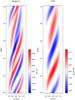 |
Fig. 2 Theoretical dynamic Stokes V (left panel) and cumulative Stokes V (right panel) profiles corresponding to the radial magnetic field maps shown in Fig. 1. |
2.2. Deconvolved longitudinal magnetic field density
A simplified form of Eq. (17) can be obtained by assuming that the local residual intensity profile is represented by a Gaussian function that does not vary across the stellar surface. This approximation, together with the weak-field assumption, is commonly made in the context of modelling stellar circular polarisation spectra (e.g. Petit et al. 2004; Petit & Wade 2012). Then, omitting λ0, the normalised residual profile becomes ![Mathematical equation: \begin{eqnarray} \dfrac{ r_I (\lambda,x)}{W_I} = \dfrac{1}{\sigma\sqrt{2\pi}}\exp{\left[-\frac{(\lambda-\Delta\lambda_R x)^2}{2\sigma^2}\right]}\cdot \end{eqnarray}](/articles/aa/full_html/2015/08/aa26318-15/aa26318-15-eq55.png) (20)Since the kernel described by this equation is known once σ and vesini are specified, it is possible to define the deconvolved longitudinal magnetic field density
(20)Since the kernel described by this equation is known once σ and vesini are specified, it is possible to define the deconvolved longitudinal magnetic field density 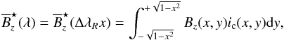 (21)in which the effect of averaging over the line profile width is taken out.
In practice,  can be obtained from the observed with the help of a suitable deconvolution algorithm. For the interpretation of
  it can also be assumed that the centre-to-limb variation of the continuum intensity is described by a linear limb-darkening law
  (22)where ε is a limb-darkening coefficient and
  .
.
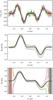 |
Fig. 3 Effect of random noise with σ = 2 × 10⁻⁴ on the Stokes V (upper panel) and CSV profiles with WI (middle panel) and 1−ℛI (bottom panel) normalisations. The thick double line shows the noise-free calculations corresponding to the rotational phase 0.125 of the model Stokes profiles discussed in Sect. 2.1. The thin lines represent profiles for different noise realisations. The |
2.3. Dynamic CSV profiles
A two-dimensional plot of the Steaks I profile variability pattern as a function of wavelength (or velocity) and rotational phase is commonly used to assess the distribution of the stellar surface inhomogeneities. Although similar plots of the Stokes V profile variation are also occasionally published (Donati et al. 1999, 2006), they could not be directly employed for obtaining information about the stellar surface magnetic field distributions. The dynamic cumulative Stokes V profiles, on the other hand, allows tracing individual magnetic spots and characterising the stellar magnetic field geometry.
An example of the dynamic CSV profiles is shown in Fig. 2. This figure presents polarisation spectra and corresponding  profiles for the model magnetic field distribution discussed in Sect. 2.1. The longitudinal positions and polarities of the four magnetic spots can be directly read out from the dynamic CSV plot. The latitudes of the spots can be deduced from the velocity span of their signatures in the profile.
2.4. Deriving CSV profiles from noisy data
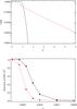 |
Fig. 4 Upper panel: cumulative distribution of |

The cumulative Stokes V profiles exhibit non-trivial noise properties. On the one hand, since the CSV spectra are computed by integrating the Stokes V signatures, some cancellation of the random noise is expected. On the other hand, the resulting noise in the CSV profiles themselves is highly correlated, leading to a qualitatively different behaviour compared to the initial Stokes V profiles. These special noise properties have to be considered when applying the CSV diagnostic to real observational data.
We investigated the noise properties of the CSV profiles with several sets of Monte Carlo simulations. First, we considered the model Stokes V spectra corresponding to the four-spot magnetic field distribution discussed in Sect. 2.1. The mean peak-to-peak amplitude of these circular polarisation profiles is ≈2 × 10⁻³. The profiles were sampled with a step of 1 km s-1, yielding about 100 spectral points across the line. A random, normally distributed noise with σ = 2 × 10⁻⁴ was added to these profiles. Typical CSV signatures resulting from the forward integration according to Eq. (14) are presented in Fig. 3. It is evident that, while the CSV spectra appear to have less random noise than the initial Stokes V profiles, they suffer from a systematic, ramping deviation from the zero line, which increases as the integration proceeds from blue to red. The bottom panel of Fig. 3 illustrates the  CSV observable normalised by the residual profile intensity 1−ℛI according to Eq. (19). The devastating impact of the noise at profile edges is apparent.
It is possible to define the CSV profiles using an alternative, backward, red-to-blue integration scheme 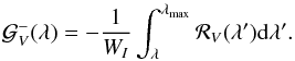 (23)This formula gives identical results to Eq. (14) in the absence of noise. When noise is present, it will lead to a systematic discrepancy similar to the one illustrated in Fig. 3, but increasing towards the blue side of the line. The overall systematic deviation from zero can be minimised by a weighted mean of the forward and backward integrations
 ![Mathematical equation: \begin{eqnarray} \overline{{\cal G}_V} (\lambda) = \dfrac{1}{W_I} \left[ w^{+} \int_{\lambda_{\rm min}}^{\lambda} {\cal R}_V(\lambda^\prime) {\rm d} \lambda^\prime - w^{-} \int^{\lambda_{\rm max}}_{\lambda} {\cal R}_V(\lambda^\prime) {\rm d} \lambda^\prime \right], \label{eq24} \end{eqnarray}](/articles/aa/full_html/2015/08/aa26318-15/aa26318-15-eq72.png) (24)where the weights w± are given by
(24)where the weights w± are given by  (25)The correction expressed by these equations is equivalent to subtracting from the original CSV profile a straight line going through 0 at λmin and
  at λmax.
Application of Eqs. (24), (25) still results in a substantially higher reduced χ2 than found for the original Stokes V profiles that are corrupted by noise. Using 106 realisations of normally distributed random noise in the absence of any background signal, we built a cumulative distribution function for the χ2 values deduced by performing integration according to Eq. (24) with associated error propagation. As shown in the upper panel of Fig. 4, integration leads to substantially higher χ2 values than the initial Stokes V profiles. For example, the 10-3 probability threshold corresponds to  for the CSV profiles compared to
  for the initial profiles.
Based on this empirical CDF of  of CSV profiles, we estimated the fraction of such profiles that will be detected above the noise level with a false-alarm probability of 10-3 or lower for the four-spot magnetic field geometry sampled at 100 equidistant rotational phases. These MC simulations were carried out for noise amplitudes in the range from 2 × 10⁻⁴ to 2 × 10⁻³, that is, 10–100% of the mean peak-to-peak Stokes V profile amplitude. Simulations were repeated 104 times for each value of the noise amplitude.
As can be seen from the lower panel of Fig. 4, the detection of magnetic field signatures using CSV profiles is less successful than with the original Stokes V spectra. Therefore, the CSV diagnostic technique does not represent a useful alternative to the widely used χ2-based Stokes V profile detection method in terms of mere field detection.
3. Observational data
For the purpose of testing the CSV diagnostic method on real data, we analysed high-resolution spectropolarimetric observations available from the Polarbase archive (Petit et al. 2014). This database provides reduced, calibrated, one-dimensional Stokes parameter spectra obtained with ESPaDOnS at CFHT and Narval at TBL of the Pic du Midi observatory. Both instruments are fibre-fed thermally stabilised echelle spectropolarimeters covering the wavelength range from 3694 to 10 483 Å in a single exposure at a resolving power of λ/ Δλ = 65 000.
As an example of the Stokes V profiles of a cool active star with a complex magnetic field we considered spectropolarimetric observations of the weak-line T Tauri star V410 Tau. This data set, discussed by Skelly et al. (2010) and Rice et al. (2011), comprises 45 Stokes V observations obtained in the span of about two weeks in January 2009. The signal-to-noise ratio of these spectra, S/N ≈ 150, is insufficient for the detection and analysis of circular polarisation signatures in individual spectral lines. Therefore, we applied the least-squares deconvolution approach (Kochukhov et al. 2010) to each spectrum, combining about 4400 spectral lines into a single high S/N ratio profile. The data were phased with the ephemeris of Stelzer et al. (2003).
We also analysed the Stokes V observations of the He-strong Bp star HD 37776. This object is known to possess a complex magnetic field, strongly deviating from an oblique dipolar geometry (Kochukhov et al. 2011). There are 27 Stokes V spectra of HD 37776, with a typical S/N ratio of 450, available in Polarbase. These data were acquired over the period of 2006–2012. We used the variable-period ephemeris of Mikulášek et al. (2008) to compute rotational phases. Since the magnetic field of HD 37776 is very strong, circular polarisation signatures are readily observable in individual spectral lines. In this paper we study the He i 6678 Å line. Its circular polarisation shows a variability pattern very similar to the He i 5876 Å line analysed by Kochukhov et al. (2011) using lower quality data.
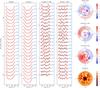 |
Fig. 5 Results of the ZDI analysis of V410 Tau. The four panels on the left side of the figure compare the observed (histogram) and theoretical (solid line) LSD Stokes I and V profiles. In these plots the spectra corresponding to different rotational phases are shifted vertically. The phase is indicated to the right of each profile. Reconstructed maps of the radial, meridional, and azimuthal magnetic field components as well as the brightness distribution are presented in the right column. The star is shown using the flattened polar projection between latitudes −60° and + 90°. The thick circle corresponds to the rotational equator. The colour bars give the field strength in kG and the brightness relative to the photospheric value. |
4. Examples of the CSV diagnostic
4.1. Weak-line T Tau star V410 Tau
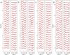 |
Fig. 6 Cumulative Stokes V profiles of V410 Tau computed from the observed (histogram) and theoretical (thick solid line) LSD circular polarisation spectra of V410 Tau shown in Fig. 5. The CSV profiles are shifted vertically according to their rotational phases similar to the Stokes V profiles in Fig. 5. The first three panels show the CSV spectra computed with a) forward integration, b) backward integration, and c) weighted mean of the backward and forward integration. The last panel d) shows the result of converting the CSV profiles in panel c) to the 1−ℛI normalisation according to Eq. (19). |
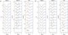 |
Fig. 7 Theoretical Stokes I, V and CSV profiles corresponding to a) the magnetic field map of V410 Tau shown in Fig. 5 and b) the same map scaled by a factor of 10. In each case the CSV column compares |
The young rapidly rotating star V410 Tau (HD 283518) exhibits ample signs of the surface magnetic activity and was targeted by a number of temperature DI studies (Hatzes 1995; Rice & Strassmeier 1996; Rice et al. 2011). These analyses revealed a persistent large polar spot and evolving temperature inhomogeneities at lower latitudes. A magnetic field was detected on V410 Tau by Donati et al. (1997). Skelly et al. (2010) reconstructed the surface magnetic field topology of this star with ZDI, finding a significant toroidal magnetic component and a complex radial field distribution. On the other hand, Carroll et al. (2012) reported a relatively simple, predominantly poloidal magnetic field structure consisting of two large polar magnetic spots with an opposite polarity. The Stokes V spectropolarimetric observations interpreted by Skelly et al. (2010) and Carroll et al. (2012) were obtained with the twin instruments (ESPaDOnS and Narval) and at practically the same time, meaning that the discrepant magnetic inversion results cannot be ascribed to the intrinsic variation of the surface magnetic field of V410 Tau.
Here we used the combined ESPaDOnS and Narval spectropolarimetric data set to reconstruct independent maps of the magnetic field topology and brightness distribution. The inversion methodology applied to V410 Tau is described in detail by Kochukhov et al. (2014). Briefly, the magnetic field of the star is represented in terms of a superposition of the poloidal and toroidal harmonic terms with the angular degree up to ℓ = 15. A penalty function prohibits unnecessary contribution of the high-order harmonic modes. A separate regularisation procedure applied to the brightness map minimises any deviation from the reference (photospheric) brightness value. We employed the analytical Unno-Rachkovsky Stokes parameter profiles (e.g. Landi Degl’Innocenti & Landolfi 2004) to approximate the local intensity and circular polarisation spectra. The brightness and magnetic field maps were recovered self-consistently from the LSD Stokes I and V profiles, adopting i = 60° and vesini = 74 km s-1.
The LSD profile fits and the resulting brightness and magnetic field maps are presented in Fig. 5. The surface distributions that we obtain are generally compatible with the maps published by Skelly et al. (2010). Similar to these authors, we find a dominant dark polar spot and numerous small-scale brightness inhomogeneities at lower latitudes. The poloidal and toroidal field components contribute 63% and 37%, respectively, to the total magnetic field energy. The field strength reaches ~1 kG locally on the stellar surface. The azimuthal field exhibits two large unipolar regions, while the radial field shows a more complex structure. The darkest areas in the brightness map do not coincide with any particular magnetic field features. We also verified that a very similar magnetic field geometry is obtained with a direct ZDI reconstruction of each magnetic field component without using the spherical harmonic formalism.
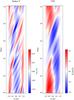 |
Fig. 8 Theoretical dynamic Stokes V (left panel) and cumulative Stokes V (right panel) profiles corresponding to the ZDI map of V410 Tau shown in Fig. 5. |
Based on the magnetic inversion results, we calculated the CSV profiles using both the observed and the ZDI model Stokes I and V spectra of V410 Tau. Figure 6 compares profiles obtained by applying Eq. (14), Eq. (23), and the weighted mean of the forward and backward integrations given by Eq. (24). It is clear that in the first and second case (Figs. 6a, b), a significant systematic deviation between the observed and theoretical CSV profiles appears due to the noise accumulation. On the other hand, systematic effects are largely brought under control in the third set of CSV profiles (Fig. 6c).
Figure 6d illustrates the effect of employing the 1−ℛI normalisation in place of the WI normalisation used elsewhere. The profiles shown in this panel directly provide the average line-of-sight magnetic field component at different longitudes on the stellar surface. However, these profiles, being morphologically similar to the spectra, are visibly distorted by the noise artefacts at the line edges.
We tested the accuracy of the CSV diagnostic with the model LSD profiles corresponding to the magnetic field map shown in Fig. 5. For clarity we disregarded the non-uniform brightness distribution and considered the line profiles for ten equidistant rotational phases. The CSV profiles were computed from the simulated observations using Eq. (14) and by performing a numerical integration of the line-of-sight magnetic field component according to the right-hand side of Eq. (17). In these calculations we used the same local non-magnetic rI profile as was adopted for the ZDI inversions. As expected, the two sets of CSV profiles agree perfectly (Fig. 7a).
The CSV method is based on the weak-field approximation, which is usually considered to be valid only for the magnetic field strengths below ~1 kG. It is useful to assess the usefulness of the cumulative Stokes V profiles for much stronger magnetic fields. To this end, we scaled all the vector components of the ZDI map of V410 Tau by a factor of 10. This increased the mean field strength from 570 G to 5.7 kG. We then repeated the direct and geometrical evaluation of the CSV profiles. The resulting spectra are compared in Fig. 7b. The two sets of profiles show only marginal discrepancies even though the characteristic magnetic field strength now significantly exceeds 1 kG. Therefore, it appears that the CSV diagnostic is usable well beyond the nominal limit of the weak-field approximation.
Using the ZDI maps of V410 Tau, we calculated variation of the Stokes parameter profiles with a dense rotational phase sampling. The resulting dynamic circular polarisation and CSV spectra are presented in Fig. 8. Unlike Fig. 2, it shows a stationary pattern (phases 0.0–0.3) in addition to features travelling across the stellar disk (e.g. phase 0.6–0.8). The travelling features are associated with the radial field spots, in particular the negative polarity spot best visible at rotational phase 0.75. The stationary features correspond to the large unipolar azimuthal field regions. This behaviour of the dynamic CSV profiles can be considered as evidence for the presence of a significant toroidal magnetic field on the stellar surface.
4.2. He-strong Bp star HD 37776
The B-type magnetic chemically peculiar star HD 37776 (V901 Ori) is known for its unusually complex double-wave longitudinal magnetic field variation (Thompson & Landstreet 1985). This behaviour indicates a large deviation of the stellar surface magnetic field topology from an oblique dipolar geometry. This object is often considered to be an example of the star with a quadrupolar magnetic field structure in the literature. Indeed, Bohlender (1994) and Khokhlova et al. (2000) derived quadrupolar magnetic geometry models for HD 37776 based on fitting the longitudinal field curve and Stokes V profile variation, respectively. However, using a more extensive set of phase-resolved spectropolarimetric observations, Kochukhov et al. (2011) showed that the circular polarisation spectra of HD 37776 cannot be fitted with an axisymmetric quadrupolar field structure. Instead, the ZDI inversion carried out in that study suggested a complex field distribution comprising a series of magnetic spots with alternating positive and negative polarity.
The high-resolution circular polarisation spectra of HD 37776 analysed here enable a straightforward verification of the ZDI results of Kochukhov et al. (2011) using the cumulative Stokes V profile diagnostic method. Figure 9 shows the Stokes V and CSV spectra centred on the He i 6678 Å line. The dynamic CSV profiles are dominated by a series of travelling features. There is no evidence of stationary structures like in the case of V410 Tau, indicating that no strong toroidal magnetic field is present. Furthermore, a careful examination of the CSV profiles allows identifying three spots with negative polarity and the same number of positive-field features. This corresponds very well to the six well-defined spots seen in the radial magnetic field map recovered with ZDI (see Fig. 5 Kochukhov et al. 2011). On the other hand, considering the dynamic CSV profiles in Fig. 9, the quadrupolar field hypothesis can be immediately ruled out. A quadrupolar magnetic field geometry with high obliquity, as required to reproduce the ⟨ Bz ⟩ variation of HD 37776, exhibits four regions of alternating field polarity along the stellar rotational equator. But Fig. 9 shows at least six regions.
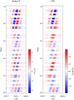 |
Fig. 9 Observed dynamic Stokes V (left panel) and cumulative Stokes V (right panel) profiles of the He i 6678 Å line in Bp star HD 37776. |
5. Summary and discussion
We examined the information content of the cumulative circular polarisation profiles and assessed their usefulness for the analysis of stellar surface magnetic fields. This work represents a further development of the idea put forward by Gayley & Owocki (2015). Starting with the weak-field approximation, we defined the new magnetic observable as a normalised integral of the Stokes V spectrum and showed its relation to the underlying surface magnetic field structure. The transformation from the Stokes V to the CSV profiles greatly simplifies the morphology of polarisation spectra and enables a direct and intuitive identification of the regions of different field polarity on the stellar surface. The CSV observable characterises the line-of-sight magnetic field component weighted by the continuum intensity and by the Doppler-shifted local residual Stokes I profile. The CSV spectrum thus provides a velocity-resolved measure of the stellar longitudinal magnetic field. Consequently, this observable is most useful for rapidly rotating stars with complex magnetic field topologies.
Using theoretical circular polarisation profile calculations and real observational data, we assessed the visibility of the surface magnetic field features in the dynamic CSV profiles. Unlike the dynamic Stokes V spectra, which can hardly be interpreted directly, the dynamic CSV profiles enable a qualitative analysis of the magnetic star spot distributions. With the help of Monte Carlo simulations, we studied the effect of random observational noise on the CSV profiles. The noise signatures in the CSV spectra are highly correlated, leading to a systematic ramping offset from a noise-free version of the line profiles. We showed that this problem can be minimised using a weighted mean of the CSV profiles computed with the forward and backward integration of the original Stokes V data. Nevertheless, the presence of correlated noise in the CSV profiles generally makes them inferior for the purpose of field detection compared to the original Stokes V spectra.
With the goal of testing the CSV magnetic field diagnostic methodology we studied the archival high-resolution circular polarisation observations of the cool active star V410 Tau and the hot magnetic star HD 37776. Both objects are rapid rotators with complex surface magnetic field topologies. For the weak-line T Tauri star V410 Tau we obtained brightness and magnetic field distributions with the help of the ZDI modelling of the least-squares deconvolved Stokes I and V profiles. The resulting magnetic map bears a close resemblance to the magnetic field topology obtained by Skelly et al. (2010) from the same data. However, our inversion results contradict the magnetic field map published by Carroll et al. (2012), whose data set was also included in our analysis. Our ZDI modelling accounted for the effect of an inhomogeneous brightness distribution on the Stokes V profiles. We have also verified that very similar magnetic field maps are obtained using the direct, pixel-based ZDI and the magnetic inversions relying on the spherical harmonic parameterisation of the stellar magnetic field. Therefore, these two aspects are unlikely to be responsible for the discrepancies of the ZDI maps presented here and in Skelly et al. (2010) on the one hand and in Carroll et al. (2012) on the other hand. It is more likely that this disagreement is rooted in the differences between the LSD (used here and by Skelly et al. 2010) and PCA (used by Carroll et al. 2012) mean polarisation profiles. A comprehensive comparative study of the LSD and PCA line-addition techniques is required to address this problem.
The dynamic CSV profiles of V410 Tau indicate the presence of a strong azimuthal magnetic field component on the stellar surface. This agrees with our ZDI results and suggests a non-negligible contribution of the toroidal magnetic field. We also used the ZDI map of V410 Tau to verify interpretation of the integral of Stokes V profiles in terms of the disk-averaged, weighted line-of-sight magnetic field component. These calculations were repeated for a scaled-up version of the stellar magnetic field geometry, demonstrating that the usefulness of the CSV diagnostic extends far beyond the nominal limit of the weak-field approximation.
For the magnetic Bp star HD 37776 we analysed the CSV dynamic spectrum of the He i 6678 Å line. The variation of its CSV profiles is clearly inconsistent with the quadrupolar magnetic field topology that has frequently been suggested for this star. On the other hand, multiple magnetic spots that can be identified in the dynamic CSV spectra of HD 37776 are consistent with the surface magnetic features in the ZDI map of this star derived by Kochukhov et al. (2011). The CSV analysis thereby confirms the complex non-quadrupolar nature of the magnetic field topology of HD 37776.
Acknowledgments
This research is supported by the grants from the Knut and Alice Wallenberg Foundation, the Swedish Research Council, and the Swedish National Space Board. The author thanks Ken Gayley for helpful discussions of the CSV diagnostic method and James Silvester for critical reading of manuscript.
References
- Aurière, M., Wade, G. A., Silvester, J., et al. 2007, A&A, 475, 1053 [NASA ADS] [CrossRef] [EDP Sciences] [Google Scholar]
- Bagnulo, S., Landi Degl’Innocenti, M., Landolfi, M., & Mathys, G. 2002, A&A, 394, 1023 [NASA ADS] [CrossRef] [EDP Sciences] [Google Scholar]
- Barnes, J. R., Collier Cameron, A., James, D. J., & Donati, J. 2000, MNRAS, 314, 162 [NASA ADS] [CrossRef] [Google Scholar]
- Bohlender, D. A. 1994, in Pulsation, Rotation, and Mass Loss in Early-Type Stars, eds. L. A. Balona, H. F. Henrichs, & J. M. Le Contel, IAU Symp., 162, 155 [Google Scholar]
- Brown, S. F., Donati, J.-F., Rees, D. E., & Semel, M. 1991, A&A, 250, 463 [NASA ADS] [Google Scholar]
- Carroll, T. A., & Strassmeier, K. G. 2014, A&A, 563, A56 [NASA ADS] [CrossRef] [EDP Sciences] [Google Scholar]
- Carroll, T. A., Strassmeier, K. G., Rice, J. B., & Künstler, A. 2012, A&A, 548, A95 [NASA ADS] [CrossRef] [EDP Sciences] [Google Scholar]
- Donati, J.-F., & Brown, S. F. 1997, A&A, 326, 1135 [NASA ADS] [Google Scholar]
- Donati, J.-F., Collier Cameron, A., Hussain, G. A. J., & Semel, M. 1999, MNRAS, 302, 437 [NASA ADS] [CrossRef] [Google Scholar]
- Donati, J.-F., Forveille, T., Cameron, A. C., et al. 2006, Science, 311, 633 [NASA ADS] [CrossRef] [PubMed] [Google Scholar]
- Donati, J.-F., Semel, M., Carter, B. D., Rees, D. E., & Collier Cameron, A. 1997, MNRAS, 291, 658 [NASA ADS] [CrossRef] [MathSciNet] [Google Scholar]
- Gayley, K. G., & Owocki, S. P. 2015, in IAU Symp. 307, eds. G. Meynet, C. Georgy, J. H. Groh, & P. Stee, 375 [Google Scholar]
- Hatzes, A. P. 1995, ApJ, 451, 784 [NASA ADS] [CrossRef] [Google Scholar]
- Hubrig, S., North, P., & Schöller, M. 2007, Astron. Nachr., 328, 475 [NASA ADS] [CrossRef] [Google Scholar]
- Johns-Krull, C. M., & Valenti, J. A. 1996, ApJ, 459, L95 [NASA ADS] [CrossRef] [Google Scholar]
- Khokhlova, V. L., Vasilchenko, D. V., Stepanov, V. V., & Romanyuk, I. I. 2000, Astron. Lett., 26, 177 [Google Scholar]
- Kochukhov, O., & Piskunov, N. 2002, A&A, 388, 868 [NASA ADS] [CrossRef] [EDP Sciences] [Google Scholar]
- Kochukhov, O., & Wade, G. A. 2010, A&A, 513, A13 [NASA ADS] [CrossRef] [EDP Sciences] [Google Scholar]
- Kochukhov, O., Bagnulo, S., Wade, G. A., et al. 2004, A&A, 414, 613 [NASA ADS] [CrossRef] [EDP Sciences] [Google Scholar]
- Kochukhov, O., Tsymbal, V., Ryabchikova, T., Makaganyk, V., & Bagnulo, S. 2006, A&A, 460, 831 [NASA ADS] [CrossRef] [EDP Sciences] [Google Scholar]
- Kochukhov, O., Makaganiuk, V., & Piskunov, N. 2010, A&A, 524, A5 [NASA ADS] [CrossRef] [EDP Sciences] [Google Scholar]
- Kochukhov, O., Lundin, A., Romanyuk, I., & Kudryavtsev, D. 2011, ApJ, 726, 24 [Google Scholar]
- Kochukhov, O., Mantere, M. J., Hackman, T., & Ilyin, I. 2013, A&A, 550, A84 [NASA ADS] [CrossRef] [EDP Sciences] [Google Scholar]
- Kochukhov, O., Lüftinger, T., Neiner, C., Alecian, E., & MiMeS Collaboration. 2014, A&A, 565, A83 [NASA ADS] [CrossRef] [EDP Sciences] [Google Scholar]
- Landi Degl’Innocenti, E., & Landolfi, M. 2004, Polarization in Spectral Lines (Kluwer Academic Publishers), Astrophys. Space Sci. Lib., 307 [Google Scholar]
- Landstreet, J. D., & Mathys, G. 2000, A&A, 359, 213 [NASA ADS] [Google Scholar]
- Marsden, S. C., Petit, P., Jeffers, S. V., et al. 2014, MNRAS, 444, 3517 [NASA ADS] [CrossRef] [Google Scholar]
- Mathys, G. 1991, A&AS, 89, 121 [NASA ADS] [Google Scholar]
- Mathys, G. 1995, A&A, 293, 733 [NASA ADS] [Google Scholar]
- Mathys, G., Hubrig, S., Landstreet, J. D., Lanz, T., & Manfroid, J. 1997, A&AS, 123, 353 [NASA ADS] [CrossRef] [EDP Sciences] [Google Scholar]
- Mikulášek, Z., Krtička, J., Henry, G. W., et al. 2008, A&A, 485, 585 [NASA ADS] [CrossRef] [EDP Sciences] [Google Scholar]
- Petit, V., & Wade, G. A. 2012, MNRAS, 420, 773 [NASA ADS] [CrossRef] [Google Scholar]
- Petit, P., Donati, J., Wade, G. A., et al. 2004, MNRAS, 348, 1175 [NASA ADS] [CrossRef] [Google Scholar]
- Petit, P., Lignières, F., Aurière, M., et al. 2011, A&A, 532, L13 [NASA ADS] [CrossRef] [EDP Sciences] [Google Scholar]
- Petit, P., Louge, T., Théado, S., et al. 2014, PASP, 126, 469 [NASA ADS] [CrossRef] [Google Scholar]
- Piskunov, N., & Kochukhov, O. 2002, A&A, 381, 736 [NASA ADS] [CrossRef] [EDP Sciences] [Google Scholar]
- Reiners, A., & Basri, G. 2007, ApJ, 656, 1121 [NASA ADS] [CrossRef] [Google Scholar]
- Rice, J. B., & Strassmeier, K. G. 1996, A&A, 316, 164 [NASA ADS] [Google Scholar]
- Rice, J. B., Strassmeier, K. G., & Kopf, M. 2011, ApJ, 728, 69 [NASA ADS] [CrossRef] [Google Scholar]
- Rosén, L., & Kochukhov, O. 2012, A&A, 548, A8 [NASA ADS] [CrossRef] [EDP Sciences] [Google Scholar]
- Shulyak, D., Reiners, A., Seemann, U., Kochukhov, O., & Piskunov, N. 2014, A&A, 563, A35 [NASA ADS] [CrossRef] [EDP Sciences] [Google Scholar]
- Skelly, M. B., Donati, J.-F., Bouvier, J., et al. 2010, MNRAS, 403, 159 [NASA ADS] [CrossRef] [Google Scholar]
- Stelzer, B., Fernández, M., Costa, V. M., et al. 2003, A&A, 411, 517 [NASA ADS] [CrossRef] [EDP Sciences] [Google Scholar]
- Thompson, I. B., & Landstreet, J. D. 1985, ApJ, 289, L9 [NASA ADS] [CrossRef] [Google Scholar]
- Wade, G. A., Donati, J.-F., Landstreet, J. D., & Shorlin, S. L. S. 2000, MNRAS, 313, 823 [NASA ADS] [CrossRef] [MathSciNet] [Google Scholar]
All Figures
|
Fig. 1 Model Stokes V (upper curves) and cumulative Stokes V (lower curves) profiles for a star with several large circular magnetic spots of different polarities. The line profiles and the spherical maps of the radial magnetic field component are shown for three different rotational phases. The phases are indicated above each line profile panel. |
| In the text | |
|
Fig. 2 Theoretical dynamic Stokes V (left panel) and cumulative Stokes V (right panel) profiles corresponding to the radial magnetic field maps shown in Fig. 1. |
| In the text | |
|
Fig. 3 Effect of random noise with σ = 2 × 10⁻⁴ on the Stokes V (upper panel) and CSV profiles with WI (middle panel) and 1−ℛI (bottom panel) normalisations. The thick double line shows the noise-free calculations corresponding to the rotational phase 0.125 of the model Stokes profiles discussed in Sect. 2.1. The thin lines represent profiles for different noise realisations. The |
| In the text | |
|
Fig. 4 Upper panel: cumulative distribution of |
| In the text | |
|
Fig. 5 Results of the ZDI analysis of V410 Tau. The four panels on the left side of the figure compare the observed (histogram) and theoretical (solid line) LSD Stokes I and V profiles. In these plots the spectra corresponding to different rotational phases are shifted vertically. The phase is indicated to the right of each profile. Reconstructed maps of the radial, meridional, and azimuthal magnetic field components as well as the brightness distribution are presented in the right column. The star is shown using the flattened polar projection between latitudes −60° and + 90°. The thick circle corresponds to the rotational equator. The colour bars give the field strength in kG and the brightness relative to the photospheric value. |
| In the text | |
|
Fig. 6 Cumulative Stokes V profiles of V410 Tau computed from the observed (histogram) and theoretical (thick solid line) LSD circular polarisation spectra of V410 Tau shown in Fig. 5. The CSV profiles are shifted vertically according to their rotational phases similar to the Stokes V profiles in Fig. 5. The first three panels show the CSV spectra computed with a) forward integration, b) backward integration, and c) weighted mean of the backward and forward integration. The last panel d) shows the result of converting the CSV profiles in panel c) to the 1−ℛI normalisation according to Eq. (19). |
| In the text | |
|
Fig. 7 Theoretical Stokes I, V and CSV profiles corresponding to a) the magnetic field map of V410 Tau shown in Fig. 5 and b) the same map scaled by a factor of 10. In each case the CSV column compares |
| In the text | |
|
Fig. 8 Theoretical dynamic Stokes V (left panel) and cumulative Stokes V (right panel) profiles corresponding to the ZDI map of V410 Tau shown in Fig. 5. |
| In the text | |
|
Fig. 9 Observed dynamic Stokes V (left panel) and cumulative Stokes V (right panel) profiles of the He i 6678 Å line in Bp star HD 37776. |
| In the text | |
Current usage metrics show cumulative count of Article Views (full-text article views including HTML views, PDF and ePub downloads, according to the available data) and Abstracts Views on Vision4Press platform.
Data correspond to usage on the plateform after 2015. The current usage metrics is available 48-96 hours after online publication and is updated daily on week days.
Initial download of the metrics may take a while.