| Issue |
A&A
Volume 580, August 2015
|
|
|---|---|---|
| Article Number | A81 | |
| Number of page(s) | 9 | |
| Section | Stellar atmospheres | |
| DOI | https://doi.org/10.1051/0004-6361/201526073 | |
| Published online | 06 August 2015 | |
The remarkably unremarkable global abundance variations of the magnetic Bp star HD 133652⋆
1 Max Planck Insitut für Extraterrestrische Physik, Giessenbachstrasse 1, 85748 Garching, Germany
e-mail: This email address is being protected from spambots. You need JavaScript enabled to view it.
2 Armagh Observatory, College Hill, Armagh, BT61 9DG, Northern Ireland, UK
3 Department of Physics and Astronomy, University of Western Ontario, London, Ontario, N6A 3K7, Canada
Received: 11 March 2015
Accepted: 8 June 2015
Abstract
Context. In recent years, significant effort has been made to understand how the magnetic field strengths and atmospheric chemical abundances of Ap/Bp stars evolve during their main sequence lifetime by identifying a large number of Ap/Bp stars with accurately known ages. As a next step, these stars should be studied individually and in detail to offer further insight into the physics of how such main sequence stars evolve.
Aims. We have obtained high resolution spectra using the ESPaDOnS spectropolarimeter and FEROS spectrograph of the chemically peculiar, magnetic Bp star HD 133652. Using these data, we present a simple magnetic field model and abundance determinations of He, O, Mg, Si, Ti, Cr, Fe, Pr, and Nd.
Methods. Abundance analysis was performed using zeeman.f, a spectral synthesis program that includes the effects of magnetic fields on line formation. The magnetic field structure is approximated as a simple, co-linear multipole expansion that reproduces the observed variations of the line-of-sight magnetic field with phase. The abundance distribution of each element was modelled using a uniform abundance in each of the two magnetic hemispheres.
Results. Using the new magnetic field measurements, we were able to refine the rotation period of HD 133652 to P = 2.30405 ± 0.00002 d. The abundance analysis reveals that the elements modelled (except He, O and Mg) are overabundant compared to the Sun; however most elements studied do not show substantial differences in the large-scale mean abundances between the two magnetic hemispheres. The individual line profiles are very complex and clearly indicate the presence of significant small-scale abundance variations on the stellar surface.
Conclusions. These data are adequate to perform a useful investigation of the magnetic field structure and abundance distribution over the stellar surface. HD 133652 is now one of a growing list of hotter Bp stars of known age for which this type of analysis has been performed.
Key words: stars: abundances / stars: chemically peculiar / stars: magnetic field
Based in part on our own observations made with the European Southern Observatory (ESO) telescopes under the ESO programme 086.D-0449(A). It is also based in part on observations carried out at the Canada-France-Hawaii Telescope (CFHT) which is operated by the National Research Council of Canada, the Institut National des Science de l’Universe of the Centre National de la Recherche Scientifique of France and the University of Hawaii.
© ESO, 2015
1. Introduction
Approximately 10% of main sequence A and B stars host magnetic fields. Most of these stars are chemically peculiar, and are referred to as Ap/Bp stars. Such stars have organised, global magnetic fields with typical strengths of order 1 kG or higher and exhibit anomalous abundances of particular elements. For example, the Fe-peak elements can be of order 102 times more abundant in Ap/Bp stars than in the Sun. The abundances of rare-earth elements (e.g. Pr and Nd) are even more drastically peculiar, with values commonly 104 times larger than the solar abundance (Ryabchikova 1991). These magnetic stars are also variable, with the magnetic field strength, spectral line strengths and shapes, and photometric brightness varying with the same rotation period. This period is typically between about one and ten days. The universally accepted model describing the observed variability is the rigid rotator model, according to which the line of sight and the magnetic field axis are inclined at angles i and β to the rotation axis, respectively (Stibbs 1950). The abundances of several elements are distributed non-uniformly over the stellar surface in a non-axisymmetric pattern about the rotation axis, so observing the Ap/Bp star at various phases during its rotation period results in detection of spectrum and brightness variability (Ryabchikova 1991). Furthermore, the magnetic field observed at different phases may lead to varying field measurements.
HD 133652 (=HR 5619) is a chemically peculiar Bp star that is a member of the Upper Cen Lup association. This means it is a star with a well-known age of log t = 7.20 ± 0.10 that has only completed about 6 ± 2% of its main sequence lifetime (Landstreet et al. 2007). Table 1 summarises the stellar and magnetic properties.
Bohlender et al. (1993) studied the mean line-of-sight magnetic field (⟨ Bz ⟩) variations using an Hβ magnetograph. They discovered that HD 133652 has a reversing field, with extrema of order −2170 and 660 G. These data, together with the Geneva photometry of Lanz et al. (1991), made the determination of a precise period of P = 2.3040 ± 0.0003 d possible. Using the projected rotational velocity (vsini) of 70 km s-1 reported by Levato (1972), they cautiously constrain the geometry of HD 133652. They find that 32°<i< 90° and β< 86°. Furthermore, based on an inaccurate value of vsini from the literature, the minimum radius of the star was estimated to be 3.2 R⊙.
Recently, Bailey et al. (2014) studied the main sequence evolution of atmospheric abundances of Ap/Bp stars by analysing several magnetic Ap/Bp stars of known age (members of open clusters or associations). HD 133652 is a member of this sample. They derived the mean abundances of a handful of elements using two spectra. For each spectrum, a uniform abundance was derived and the average between the two results was reported. They clearly show that the atmosphere of HD 133652 is overabundant in the Fe-peak elements of Ti, Cr and Fe by more than 100 times compared to the solar ratios. The rare earth elements of Pr and Nd are of order 104 times more abundant than in the Sun. HD 133652 is certainly a He-weak star as well, as the abundance of He is a factor of 100 below the abundance found in the Sun.
Over the past five years, substantial effort has been made to analyse, in detail, the hotter Bp stars with strong magnetic fields (see for example studies of HD 318107, HD 133880, and HD 147010; Bailey et al. 2011, 2012; Bailey & Landstreet 2013b, respectively). This paper adds HD 133652 to that growing list, in which we discuss our efforts to model the magnetic field and derive a more detailed atmospheric abundance distribution based on high-dispersion spectropolarimetric observations that are well spaced throughout the rotation cycle of this star. The following section describes the spectroscopic and spectropolarimetric observations used and how the magnetic field measurements are made; Sect. 3 reports on the improvement of the accuracy of the rotation period; Sect. 4 discusses the spectrum modelling technique; Sect. 5 describes the abundance models; and Sect. 6 discusses and summarises the paper.
Summary of the stellar and magnetic properties of HD 133652.
Log of available spectra for HD 133652.
2. Observations and magnetic field measurements
We have acquired a total of nine spectra of HD 133652 over three observing runs. Six spectra were obtained using the cross-dispersed echelle spectropolarimeter ESPaDOnS, located at the 3.6 m Canada-France-Hawaii Telescope (CFHT). ESPaDOnS has the ability to observe stars in all four Stokes parameters (I,Q,U,V) with a spectral range from about 3690−10 481 Å.We have four polarised spectra in Stokes I and V and two unpolarised spectra in just Stokes I. The resolving powers R are about 65 000 and 80 000 for the polarised and unpolarised spectra, respectively.
Three spectra were obtained using the FEROS spectrograph located at the European Southern Observatory (ESO) La Silla 2.2 m Telescope. FEROS is a bench-mounted echelle spectrograph covering a spectral range from about 3600 to 9200 Å with R ≃ 48 000.
The data are summarised in Table 2. The columns list the instrument used, Julian Date of the start of each observation, phase (see Sect. 3), total exposure time, estimated signal-to-noise ratio (S/N) per 1.8 km s-1 velocity bin at 5000 Å, ⟨ Bz ⟩ measurements (see below), spectral resolution, wavelength coverage and radial velocity (RV). The RVs are determined by measuring the wavelength shifts of a set of spectral lines with low Zeeman sensitivity. These values are then tested when fitting a synthetic spectrum to the observations during the abundance analysis (see Sect. 5). The agreement between these two methods is approximately 1 km s-1 and we therefore adopt this as our estimated uncertainty.
2.1. Longitudinal magnetic field measurements
To measure the longitudinal magnetic fields ⟨ Bz ⟩ of the ESPaDOnS Stokes V spectra, we used the method of least squares de-convolution (LSD; Donati et al. 1997). For each spectrum, a mean line profile is obtained by combining all the metallic lines from an appropriate line list that is acquired from the Vienna Atomic Line Database (VALD; Kupka et al. 2000, 1999; Ryabchikova et al. 1997; Piskunov et al. 1995). The generic list chosen has an appropriate Teff and log g with sufficiently enhanced Fe-peak and rare-earth elements to reflect the abundance analysis (see Sect. 5). The longitudinal magnetic field was measured from the first order moment of the Stokes V profile according to the equation: ![Mathematical equation: \begin{equation} \langle \mathit{B}_z \rangle = \frac{-2.14 \times 10^{12}}{\lambda z c }\frac{\int{(vV(v){\rm d}v}}{\int{[I_{c}-I(v)]{\rm d}v}}, \label{b_eq} \end{equation}](/articles/aa/full_html/2015/08/aa26073-15/aa26073-15-eq46.png) (1)where ⟨ Bz ⟩ is in G, z is the mean Landé factor, λ is the mean wavelength of the weighted LSD line in Å, and v is the velocity within the LSD profile in km s-1. We chose the limits of integration upon visual inspection to ensure that the entire profile was used without introducing unneccesary noise from the continuum. Errors were computed by propagating them in the usual way. The sixth column of Table 2 lists the ⟨ Bz ⟩ measurements.
(1)where ⟨ Bz ⟩ is in G, z is the mean Landé factor, λ is the mean wavelength of the weighted LSD line in Å, and v is the velocity within the LSD profile in km s-1. We chose the limits of integration upon visual inspection to ensure that the entire profile was used without introducing unneccesary noise from the continuum. Errors were computed by propagating them in the usual way. The sixth column of Table 2 lists the ⟨ Bz ⟩ measurements.
2.2. Mean surface magnetic field modulus
Bailey (2014) demonstrate that reliable mean surface magnetic field (or mean field modulus) ⟨ B ⟩ measurements can be obtained for stars with projected rotational velocities up to about 50 km s-1. Unfortunately, HD 133652 rotates near this threshold (vsini= 45 ± 2 km s-1) and has very coarse line profiles that are the result of small-scale structure and inhomogeneous distribution of elements on the stellar surface. Nevertheless, applying the methods outlined by Bailey (2014), we are able to extract an upper limit for the value of ⟨ B ⟩ of about 9 kG. Although we are unable to study how ⟨ B ⟩ may vary throughout the rotation cycle of the star, this upper limit is somewhat useful in attempting to adopt an adequate magnetic field model to use for abundance analysis (see Sect. 4).
3. Period refinement
Bohlender et al. (1993) used nine Hβ⟨ Bz ⟩ measurements together with Geneva U, B and V photometric variations from Lanz et al. (1991) to unambiguously determine a rotation period of P = 2.3040 ± 0.0003 d. This period seems to phase the light curves and magnetic data together reasonably well; however, Bohlender et al. (1993) point out that a phase shift between the extrema of the light and magnetic curves of slightly less than 0.1 cycles is present.
Photometric data also exists for HD 133652 in the Hipparcos catalogue (Perryman et al. 1997). From the catalogue, a best-fit period of 2.30366 d is suggested, without comment on error or uniqueness. The overall fit to the Hipparcos data is reasonable. The amplitude of the variations in the Hipparcos data is only of order 4σ, with some obvious outliers. From these data, we conclude that the available data do not establish a unique period and a larger, dedicated programme of high precision photometry would be necessary to uniquely define the photometric period.
The best way to determine the rotation period of HD 133652 is with a series of ⟨ Bz ⟩ observations, with sufficient spacing, because the field variations are very large compared to the usual uncertainties. We have ⟨ Bz ⟩ measurements spanning nearly 25 years; however, the datasets were collected using different techniques (i.e. Hβ versus metallic line ⟨ Bz ⟩ measurements) and it is not at all clear that the data should be on the same scale. Fortunately, the four new data points from ESPaDOnS lie within the range of the Hβ data, which suggests that there is perhaps no large scale change between the two kinds of measurements. Assuming that this is the case, we combine both datasets to attempt to improve the period. The best-fit period is judged by the reduced χ2 of a sine wave fit to the ⟨ Bz ⟩ variations. We find only one acceptable period P = 2.30405 ± 0.00002 d with a reduced χ2 of the fit to all the Hβ and new ESPaDOnS data of 1.9. This is remarkable agreement considering the difference between the two instrumental systems in which the ⟨ Bz ⟩ measurements were made. We have phased all data according to the ephemeris:  (2)where we adopt a zero point that corresponds to the minimum in the ⟨ Bz ⟩ variations.
Figure 1 shows the ⟨ Bz ⟩ variations (top panel) and the Hipparcos photometric variations (bottom panel). The ⟨ Bz ⟩ data are in satisfactory agreement with one another, and the Hipparcos data appear to be fit just as well with this improved period as with the previously favoured Hipparcos period. We note also that the phase shift reported by Bohlender et al. (1993) between the magnetic and photometric extrema of less than about 0.1 cycles still exists with this new period.
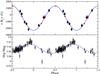 |
Fig. 1 ⟨ Bz ⟩ and Hipparcos photometry variations of HD 133652. Top: ⟨ Bz ⟩ LSD measurements (red triangles) and the Balmer line measurements from Bohlender et al. (1993, filled circles with error bars). The solid blue line is the best-fit magnetic field variations (see Sect. 4.1). Bottom: the Hipparcos photometry variations with rotational phase. The dotted blue line is the best-fit sinusoid to the observations. |
4. Spectral modelling technique
The magnetic spectrum synthesis program zeeman.f was used to model the spectrum of HD 133652 (Landstreet 1988; Landstreet et al. 1989). This program computes an emergent spectrum for a specified Teff and log g, with a prescribed magnetic field strength and geometry. The magnetic field geometry is described as a colinear dipole, quadrupole and octupole with specified angles between the rotation axis and magnetic field, β, and between the rotation axis and line-of-sight, i. The parameters for the magnetic field model are computed based upon ⟨ Bz ⟩ (and when possible ⟨ B ⟩) variations as a function of phase (see Landstreet & Mathys 2000). Over the stellar surface, either a uniform abundance or an abundance distribution varying with magnetic co-latitude can be assumed. Thus, both the magnetic field model and the abundance model assume axi-symmetry around the axis of the magnetic dipole component of the field.
zeeman.f assumes local thermodynamic equilibrium (LTE) and uses a grid of ATLAS9 model atmospheres to interpolate an appropriate atmospheric model. The atomic data required for spectrum synthesis are taken from the VALD database, and line blending is taken into account by adding the polarised line opacities prior to solving the equation of radiative transfer. More detailed descriptions of how zeeman.f works can be found in the literature (e.g. Landstreet 1988; Bailey et al. 2011).
The abundance distribution is assumed to be axisymmetric about the magnetic axis. The abundance variation with magnetic latitude is specified with uniform abundances in up to six rings with equal spans in co-latitude. The abundance of one element can be varied at a time and up to ten phases of observations in Stokes I can be fit simultaneously. As output, zeeman.f provides optimal values for vsini and RV, and produces output in all Stokes parameters (I,Q,U,V). This provides a coarse model of the abundance variations with magnetic latitude, which are quite schematic compared to the more detailed mapping using magnetic doppler imaging (MDI) done by, for example, Kochukhov et al. (2004).
A magnetic field model
The longitudinal magnetic field variations shown in Fig. 1 can be described by a simple sinusoidal variation of the form,  (3)The best-fit to the data produces a reduced χ2 of 1.41 with coefficients B0 = −494 ± 17 G, B1 = 1830 ± 26 G and φ0 = 0.253 ± 0.001.
The longitudinal magnetic field variations provide limited information about the details of the magnetic field structure. The sinusoidal nature of the ⟨ Bz ⟩ variations is indicative of a predominantly dipolar field structure. This does not, however, preclude the possibility that the field structure is substantially more complex than a global dipole distribution.
The longitudinal magnetic field of HD 133652 is reversing, with both the positive and negative magnetic hemispheres being clearly observed through the rotation cycle of the star. This indicates that, in the context of the rigid rotator model, i + β> 90°. To constrain i, we can use the relationship 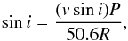 (4)where P is the rotation period in days, vsini is in km s-1 and R is the stellar radius measured in solar radii. To use this expression, an estimate of the stellar radius must be made. This can be done either by using the luminosity and Teff or the log g and mass reported in Table 1. The stellar radius is then estimated to be R = (2.17 ± 0.24) R⊙. Using the period found in this study of P = 2.30405 d, we find that the rotation axis inclination is i = 71 ± 8°.
From our calculation of i, we can then compute β from the expression 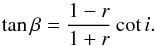 (5)The r parameter is the ratio of the ⟨ Bz ⟩ extrema (see Preston 1967, 1970). The obliquity of the magnetic axis is β = 68 ± 12°.
An appropriate magnetic field model is necessary before performing abundance analysis. HD 133652 rotates too quickly to observe Zeeman splitting in individual spectral lines, which limits what is known about the surface integrated magnetic field ⟨ B ⟩ (see Sect. 2.2). Therefore, the main criteria we require for the magnetic field is that it should reproduce the observed ⟨ Bz ⟩ variations reasonably well, that the spectral line profiles in Stokes I are not too broad compared to observations, and that the circular polarisation signatures (Stokes V) are satisfactorily modelled.
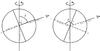 |
Fig. 2 Adopted geometry for HD 133652. The vertical axis is the rotation axis. The angle between the rotation axis and the line of sight is i = 71° and the angle between the rotation axis and magnetic field axis is β = 68°. The solid line that is perpendicular to the labelled magnetic axis indicates how the star was divided for abundance analysis. The left panel depicts the orientation when the line-of-sight is closest to the negative magnetic pole (φ = 0.0). The right panel depicts the orientation when the line-of-sight is closest to the positive magnetic pole (φ = 0.5). |
To achieve the first of the criteria, the polar field strength of the dipole is calculated using the adapted expression from Preston (1967),  (6)In this expression,
  is the maximum value of the longitudinal magnetic field and u is the limb-darkening coefficient which we have estimated to be about 0.4 based on the appropriate ATLAS9 model atmosphere for a star of Teff = 13 000 K and log g = 4.3. To calculate an appropriate polar field strength, we opted to use the average of the amplitude of the best-fit sinusoidal variations because this seems representative of the maximum value that the longitudinal field would achieve when considering both the Balmer line and metallic datasets together. This results in a dipolar field strength of 6100 G. The variation of ⟨ Bz ⟩ with phase predicted by this model is very similar to that shown in Fig. 1. The very satisfactory fit appears to support the assumed axi-symmetry of the field model.
To judge the second criterion, we note that the rotational broadening, which dominates the spectral line broadening, is first determined from measurements of magnetically insensitive lines to serve as a standard. We then evaluate the field by comparing computed synthetic line profiles to magnetically sensitive lines. A model produced in this manner is not unique, but should ensure that the model fits are mostly sensitive to chemical abundance.
To satisfy the final criterion of comparison with the observed Stokes V profile, we started with a simple dipole. Compared to the Stokes V signatures shown in Fig. 3 for the four phases for which we have data, the dipole produces V signatures in the Fe ii line at 5018 Å that are similar in amplitude and shape to those at phases 0.183 (between negative pole passage and “crossover” where we see the field from the side) and 0.732 (very close to the crossover phase where the field is equal to zero). However, the predicted signatures have much larger amplitude than the observed ones at phases 0.270 (the other crossover phase, again where ⟨ Bz ⟩ ≈ 0) and at 0.516, very close to the nearest approach of the line of sight to the positive magnetic pole.
The much smaller relative amplitude of the signal in V at phase 0.516 compared to that at phase 0.183 (or at passage of the negative pole) can be reproduced qualitatively with the assumed model by introducing a linear quadrupole component aligned with the dipole in such a way that both components have the same sign at the negative pole. This component has the effect of enhancing the local field at the negative pole and diminishing it near the positive pole, leading to a considerably diminished field amplitude at phase 0.516.
However, the striking difference between the V signals at phases 0.270 and at 0.732, which are almost exactly equally distant in phase from the two pole passages, cannot be reproduced by any axisymmetric field geometry. It can be shown that for an axisymmetric field geometry, the V signal, for an isolated line, at some phase difference Δφ from a nearest approach to a pole, is equal to that at the phase −Δφ from the same phase of pole passage, after reflection about both the V = 0 line and about the central wavelength of the line studied. This is clearly not the case for the two crossover spectra of HD 133652. This same weakness of the V signature at phase 0.27 compared to that at 0.73 is observed in the spectral lines of other abundant elements such as Ti and Cr, and is thus very probably not due to anomalous sampling of the magnetic field by a very patchy surface distribution of Fe. These observations clearly reveal that the magnetic field cannot be accurately approximated by any axisymmetric field geometry. It is noteworthy that this result does not emerge from the ⟨ Bz ⟩ curve, but only from a detailed examination of the Stokes V signatures as functions of phase.
In this situation, we simply adopt a magnetic field model that very roughly reproduces the observed circular polarisation features. Since our previous experiments indicate that the results of abundance analysis are not very sensitive to the details of the magnetic field model, but mainly to the overall magnitude of the field, we do not believe that this rough approximation leads to substantial increases in the uncertainty of our results. Our adopted magnetic field structure is a simple combination of dipole and quadrupole field, with i = 71°, β = 68°, Bd = −6100 G and Bq = −3050 G at the negative magnetic pole. The ⟨ Bz ⟩ variations predicted by this model are shown in Fig. 1, and the variations of Stokes V in the vicinity of the 5018 Å line of Fe ii are compared to the observed circular polarisation data in Fig. 3. We adopt this field structure for the abundance analysis which follows.
Abundance distributions of elements studied.
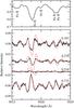 |
Fig. 3 Phase-resolved Stokes V spectra for HD 133652. The solid black lines are the observed spectra and the dashed red lines are the synthetic spectra using the adopted field geometry (see Table 1). The rotational phases are labelled. The top panel is the Stokes I signature for the same spectral window for one of the ESPaDoNS observations (φ = 0.183). Note that the negative and positive magnetic poles pass closest to the line of sight at phases 0.0 and 0.5, respectively. |
5. Abundance distribution of elements
5.1. A suitable chemical abundance model
Determining a suitable abundance distribution model requires experimentation and visual evaluation. We have nine spectra with generally good phase coverage of the rotation cycle of HD 133652. Note, however, that we are lacking coverage near the negative extremum of the ⟨ Bz ⟩ field curve and have more spectra covering the positive magnetic hemisphere. Nevertheless, the sampling is adequate to explore multi-ring models, where the abundances are allowed to vary with magnetic latitude when we search for the best-fit model for each element. zeeman.f was developed for stars like 53 Cam in which both magnetic hemispheres are clearly visible during the rotation cycle with large differences in the mean abundances between the hemispheres (Landstreet 1988). HD 133652 would seem to fulfill these same criteria. Therefore, we began our analysis with a three ring model (constant abundances within rings that span 60° in latitude). Unfortunately, using this model we were unable to achieve convergence to the same solution when different initial abundances were assumed. This was most noticeable for the magnetic equator (60°–120°) where the calculated abundance would be significantly different depending upon the initial conditions. We eventually concluded that the ring encompassing the magnetic equator was likely not well modelled with a uniform abundance.
We therefore attempted a two ring model (constant, but different, abundances within the positive and negative magnetic hemispheres). We also experimented with a four ring model (two rings of equal span in latitude in each hemisphere). We found that the four ring model predicted the same abundances as the two ring model for both hemispheres. Our conclusion is that a two ring model was adequate to describe the abundance variations over the stellar surface. Figure 2 sketches the adopted field geometry for HD 133652, including how the star was divided for the abundance analysis.
We obtained the best-fit models from various spectral windows of five chosen spectra that were well spaced in phase. To estimate the uncertainties, we used the standard deviation of the abundances found in different spectral windows. The fact that we can fit all spectral lines reasonably well gives us confidence that our adopted model is meaningful in describing the large-scale abundance variations over the stellar surface of HD 133652.
Both the FEROS and ESPaDOnS spectra have large wavelength coverages, meaning that multiple lines of many elements of various strengths can be modelled. Using our data, we are able to obtain first approximations to the abundance distributions for He, O, Mg, Si, Ti, Cr, Fe, Pr and Nd.
We list the mean abundances for both the positive and negative magnetic hemisphere in Table 3. Also listed are the uncertainties, solar abundance ratios from Asplund et al. (2009) and the number of lines modelled. For elements that only have one modelled line, we estimate the uncertainty to be of order ±0.3 dex. The quality of fits is shown in Fig. 4 for all of the available spectra. Note that the spectral line profiles of several elements (especially Ti) are very complex, possibly hinting towards detailed small scale structure on the stellar surface. As a result, the fits to some spectral lines in the process of modelling are very coarse and should be considered when evaluating the quality of fits. Each element is discussed in detail below.
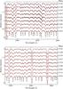 |
Fig. 4 Synthetic spectra of two spectral windows for HD 133652. The solid black lines are the observed spectra and the dashed red lines are the synthetic spectra. The spectra were shifted vertically for clarity and the rotational phases are labelled on the right. |
5.2. Helium
The triplet lines of He i at 5876 Å are the strongest in the spectrum and the only helium lines suitable for modelling. Fitting these lines suggest that the abundance of helium is uniform over the stellar surface, with an abundance that is about 100 times less than in the Sun. This abundance was also tested on the He i triplet at 4471 Å, however, these lines are not unambiguously detected. Nevertheless, the upper limit that could be derived from these lines agrees with the adopted abundance. HD 133652 is a He-weak star.
5.3. Oxygen
There are two sets of O i lines that are useful to model: the nine lines at 6155-56-58 Å and the triplet at 7771-74-75 Å. The former lines are weaker and blended with lines of Pr, whereas the latter are stronger and unblended, but usually exhibit non-LTE effects. Nevertheless, the abundances deduced from both sets of lines agree well with one another and suggest an abundance that is 0.6 dex and nearly 0.8 dex lower than the solar value in the negative and positive magnetic hemispheres, respectively.
5.4. Magnesium
The abundance distribution for magnesium was calculated from one line of Mg ii at 4481 Å. This line is fit well in all spectra and suggests a uniform abundance over the stellar surface that is about 10 times lower than in the Sun.
5.5. Silicon
Several lines of Si ii are suitable for modelling. These include lines at 4621, 5041, 5055-56, 5955 and 5978 Å. The lines at the two longer wavelengths, as well as λ4621 are well modelled at all phases; however, the fits to the line at 5041 Å and the doublet at 5055-56 Å are less satisfactory, most notably in the λ5041 line which is modelled systematically too weak at some phases. This can be seen in Fig. 4. The fits to these lines suggest large-scale abundance variations between magnetic hemispheres by only a factor of about 3. Both hemispheres are overabundant in Si compared to the Sun, with the negative magnetic hemisphere being of order 25 times higher than in the Sun, compared to about 8 times in the positive magnetic hemisphere.
We note that the three Si iii lines at 4552, 4567 and 4574 Å are present in all spectra and require an enhanced abundance that is 1 dex larger than what is derived from lines of Si ii to be adequately modelled. The discrepancy is most noticeable in λ4552, whereas the two longer wavelength lines of Si iii are arguably adequately modelled using the abundance derived from lines of Si ii at some phases (see Fig. 4). We do note, however, that the two longer wavelength Si iii lines are equally well modelled with the enhanced abundance. This result is consistent with the reports of Bailey & Landstreet (2013a), who suggest that this discrepancy between the abundances found from lines of Si ii and Si iii is most likely attributed to strong vertical stratification of Si in the stellar atmosphere.
5.6. Titanium
The spectra are rich with lines of Ti ii. We chose to model lines at 4563 and 4572 Å simultaneously, and test the calculated abundance distribution with lines at 4798 and 4805 Å. The adopted abundance distribution does an adequate job modelling the lines of Ti at most phases. We point out that this element in particular exhibits very complex (“ratty”) line profiles at all rotational phases that are poorly modelled and indicate the presence of significant small-scale structure on the stellar surface. This is easily seen in Fig. 4, where the redward wings in the latter phases are too strong in the synthetic spectra compared to the observations (e.g. phases 0.684, 0.732 and 0.816). In addition, nearest the negative magnetic pole (phase 0.183), the modelled blueward wing is too strong compared to what is observed and the cores of the synthetic lines for phases 0.248 and 0.270 are too strong.
This Fe-peak element shows modest global abundance variations over the stellar surface. In the negative magnetic hemisphere, Ti is more than 50 times higher than in the Sun and in the positive magnetic hemisphere about 20 times overabundant.
5.7. Chromium
We chose to model the abundance distribution of Cr based on six lines of Cr ii that were fit simultaneously: 4539, 4555, 4558, 4565, 4588 and 4592 Å. The quality of fit for some of these lines of Cr is shown in Fig. 4. Most lines are well modelled at all phases; however, models of some lines, such as λ4589 are too weak at some phases, except near the closest approach to the positive magnetic pole. The global distribution is clearly more complex than our simple chemical model. Like titanium, the line profiles for a significant number of Cr lines are complex and poorly modelled with our synthetic spectra (see Fig. 4). It appears that this Fe-peak element may also exhibit significant small-scale variations over the stellar surface.
Chromium is clearly overabundant compared to the Sun in both magnetic hemispheres. The global abundance variations of this element are not large and Cr has a roughly uniform abundance that is of order 100 times larger than the solar abundance ratio.
5.8. Iron
There are numerous lines of Fe ii that are useful for modelling throughout the spectrum. We fit multiple lines between 4530−4630 and 5000−5100 Å. Our final abundance distribution is the result of fitting several lines of different strengths simultaneously within these two spectral windows. Fe is uniformly abundant over the stellar surface, with an abundance that is about 1.4 dex above the solar value.
Some of the stronger lines of Fe ii (e.g. λ4583) show a tendency to be computed stronger than what is observed at some rotational phases. We also note that the spectral lines that are a blend of Cr ii and Fe ii are generally modelled too strong compared to observations. This possibly indicates that our adopted abundances may be too high for one, or both, of these Fe-peak elements. Experiments where we favour fitting the stronger lines of Fe over the weaker lines create more reasonable fits to these blended lines and the strong Fe lines, but systematically predicts line strengths for the clean, unblended weaker lines of Fe that are too weak. This may suggest that vertical stratification of Fe throughout the atmosphere is important (Bagnulo et al. 2001). We also note, that like the other Fe-peak elements, that the line profiles of iron are also “ratty,” but to a lesser extent than what is seen with Ti.
5.9. Praseodymium
We used three lines of Pr iii at 6160, 6161 and 7781 Å to model the abundance distribution of this element. This rare-earth is fit reasonably well at all phases with a uniform abundance that is at least 104 times more abundant than in the Sun.
5.10. Neodymium
The abundance distribution of Nd was derived from five lines of Nd iii at 4911-12-14, 5050 and 6145 Å. There is measurable scatter between the abundances derived from different lines of Nd iii, with a single abundance not adequately fitting all the lines modelled for a single spectrum. Regardless, Nd is about 104 times higher in abundance than the solar value and is possibly more abundant in the negative magnetic hemisphere than the positive one.
6. Discussion and conclusions
This paper presents an analysis of the magnetic Bp star HD 133652, which is part of a growing list of magnetic stars in open clusters of known age that have been studied in detail. The goal of this study was to establish a suitable magnetic field model and calculate the abundance distribution of several elements common to Ap/Bp stars.
Having completed only 6% of its main sequence lifetime, HD 133652 is a very young hot magnetic Bp star with Teff = 13 000 K. It is a member of the Upper Cen Lup association and therefore has a known age of log t = 7.20. The rotation period, computed based in the line-of-sight magnetic field variations (⟨ Bz ⟩ varies between about −2200 and 1500 G), is 2.3045 d and it has vsini of 45 km s-1. The global magnetic field strength is less than 9 kG, which was estimated based upon the broadening in magnetically sensitive lines (see Bailey 2014).
The elemental abundances of this star were already studied in some detail by Bailey et al. (2014). In their paper, uniform abundances were calculated for He, O, Mg, Si, Ti, Cr, Fe, Pr and Nd in the context of searching for atmospheric abundance evolution in Ap stars of 3.5 ± 0.5 M⊙. However, no effort was made to characterise how the abundances may vary with latitude over the stellar surface and only a very simple dipolar field was used in the abundance analysis with a magnitude that reflected approximately three times the root mean square of the line-of-sight magnetic field strength.
The magnetic field structure that we use for abundance analysis is a simple, low-order multipole expansion that consists of dipole and quadrupole components. This model was established based upon the observed variations with phase of ⟨ Bz ⟩ as well as the available circular polarisation spectra. In addition to the strengths of the magnetic field components, we are also able to establish the angles between the line-of-sight and rotation axis (i) and between the rotation axis and the magnetic field axis (β). As is the case with these simple models, we are only able to provide a very coarse description of the true magnetic field structure. Nevertheless, this model reproduces the observed variations in ⟨ Bz ⟩ well (see Fig. 1), but struggles to adequately reproduce the Stokes V signatures at all phases (see Fig. 3). This is because the field of HD 133652 is clearly not axisymmetric (see Sect. 4.1). Nevertheless, this model (see Table 1 for details) is sufficient to perform an abundance analysis to first order.
Nine spectra, reasonably well spaced throughout the rotation cycle of the star, were available to model the abundance distribution of HD 133652. Several models were considered before settling upon a two ring model in which the abundances in each magnetic hemisphere are considered uniform, but different from one another. As expected, most elements have decidedly different abundances than in the Sun. The Fe-peak elements of titanium, chromium and iron, as well as Si, are all more abundant that in the Sun. Other than Fe, which is uniformly distributed over the stellar surface, the other elements may be slightly more abundant in the negative magnetic hemisphere; however, the global abundance variations are insignificant when the uncertainties in these measurements are considered. He, O and Mg were all roughly uniformly distributed over the stellar surface with abundances that are lower than the solar values. Most impressive was He, which is 100 times less abundant than in the Sun. The rare-earth elements Pr and Nd have abundances that are about 104 time higher than in the Sun. Pr has an approximately uniform abundance over the stellar surface, whereas Nd may be more abundant in the negative magnetic hemisphere.
A comparison between the abundances derived in this paper to those of Bailey et al. (2014) reveal reasonably good agreement within estimated uncertainties. This is somewhat surprising because Bailey et al. (2014) made no effort to establish a reasonably accurate magnetic field model. A recent study by Bailey et al. (2015) of the southern magnetic standard star HD 94660 also indicates that the exact choice of magnetic field model is not as important as simply including the effects of the magnetic field when performing an abundance analysis. This is potentially a very important result that requires more rigorous testing because it implies that detailed knowledge of the magnetic field structure is not necessary to derive usefully accurate global abundances for magnetic stars.
The fact that HD 133652 shows very little global abundance variations over the stellar surface is a surprising result. For the more well studied cooler Ap stars, in which both magnetic poles are clearly visible throughout the rotation cycle of the star, large scale abundance variations are observed from one pole to another (e.g. 53 Cam; Landstreet 1988). Only a handful of Bp stars have been studied in any detail, some of which have similar effective temperatures to HD 133652. For example, HD 147010 (Teff = 13 000 K; Bailey & Landstreet 2013b) has only the negative magnetic hemisphere observable, but substantial differences in the abundances of Fe-peak and rare-earth elements are measured between the negative magnetic pole and magnetic equator. HD 133880 (Teff = 13 000 K; Bailey et al. 2012) also has a reversing field where both magnetic hemispheres are observed; however, it is a significantly faster rotator with vsini = 103 km s-1. This star also shows significant abundance variations between one pole to another in Fe-peak and rare-earth elements. Another Bp star with an effective temperature around 13 000 K is HD 45583 (Semenko et al. 2008). This star also has a reversing field; however, its magnetic field variations have a clearly quadrupolar component, as evident in the longitudinal magnetic field variations with phase. The line profiles in HD 45583 show significant variability with phase and, like HD 133652, the derived abundances for the Fe-peak and rare-earth elements appear to suggest little global abundance variations, though the line profiles do not look as messy. Obviously, no conclusions can be made from these comparisons, but it is interesting that in just a handful of studies that similarities and differences can already be readily identified. Note also that it is common to refer to the hotter Bp stars simply as Ap, grouping the entire set of magnetic main sequence stars that span effective temperatures from about 7000 to 15 000 K in one stellar classification. Although Bp stars share many characteristics in common with the cooler Ap stars, as more detailed analyses are performed, it is important to make the distinction between these two classes, which will make it easier to establish the differences and commonalities between them. For instance, above about 13 000 K, some Bp stars exhibit these complex “ratty” line profiles that are not seen in the cooler Ap stars. More of these stars must be studied to help ascertain if small-scale abundance variations are perhaps more prevalent than global, large-scale variations in some Bp stars.
The magnetic field of HD 133652 is reversing, with both magnetic hemispheres clearly observable, and is not axisymmetric. The star also has complex line profiles that reveal the presence of significant small scale-structure, regardless of the large vsini. As a result, this star is an ideal candidate for Magnetic Doppler Imaging (MDI) such as the models by Kochukhov et al. (2004). This would require a large observing campaign to obtain sufficient spatial resolution in all four Stokes parameters.
Acknowledgments
J.D.L. acknowledges financial support from the Natural Sciences and Engineering Research Council of Canada.
References
- Asplund, M., Grevesse, N., Sauval, A. J., & Scott, P. 2009, ARA&A, 47, 481 [NASA ADS] [CrossRef] [Google Scholar]
- Bagnulo, S., Wade, G. A., Donati, J.-F., et al. 2001, A&A, 369, 889 [NASA ADS] [CrossRef] [EDP Sciences] [Google Scholar]
- Bailey, J. D. 2014, A&A, 568, A38 [NASA ADS] [CrossRef] [EDP Sciences] [Google Scholar]
- Bailey, J. D., & Landstreet, J. D. 2013a, A&A, 551, A30 [NASA ADS] [CrossRef] [EDP Sciences] [Google Scholar]
- Bailey, J. D., & Landstreet, J. D. 2013b, MNRAS, 432, 1687 [NASA ADS] [CrossRef] [Google Scholar]
- Bailey, J. D., Landstreet, J. D., Bagnulo, S., et al. 2011, A&A, 535, A25 [NASA ADS] [CrossRef] [EDP Sciences] [Google Scholar]
- Bailey, J. D., Grunhut, J., Shultz, M., et al. 2012, MNRAS, 423, 328 [NASA ADS] [CrossRef] [Google Scholar]
- Bailey, J. D., Landstreet, J. D., & Bagnulo, S. 2014, A&A, 561, A147 [NASA ADS] [CrossRef] [EDP Sciences] [Google Scholar]
- Bailey, J. D., Grunhut, J., & Landstreet, J. D. 2015, A&A, 575, A115 [NASA ADS] [CrossRef] [EDP Sciences] [Google Scholar]
- Bohlender, D. A., Landstreet, J. D., & Thompson, I. B. 1993, A&A, 269, 355 [NASA ADS] [CrossRef] [Google Scholar]
- Donati, J.-F., Semel, M., Carter, B., Rees, D., & Collier Cameron, A. 1997, MNRAS, 291, 658 [NASA ADS] [CrossRef] [MathSciNet] [Google Scholar]
- Kochukhov, O., Bagnulo, S., Wade, G. A., et al. 2004, A&A, 414, 613 [NASA ADS] [CrossRef] [EDP Sciences] [Google Scholar]
- Kupka, F., Piskunov, N. E., Ryabchikova, T. A., Stempels, N. C., & Weiss, W. W. 1999, A&A, 138, 119 [Google Scholar]
- Kupka, F. G., Ryabchikova, T. A., Piskunov, N. E., Stempels, H. C., & Weiss, W. W. 2000, Balt. Astron., 9, 590 [NASA ADS] [Google Scholar]
- Landstreet, J. D. 1988, ApJ, 326, 967 [NASA ADS] [CrossRef] [Google Scholar]
- Landstreet, J. D., & Mathys, G. 2000, A&A, 359, 213 [NASA ADS] [Google Scholar]
- Landstreet, J. D., Barker, P. K., Bohlender, D. A., & Jewison, M. S. 1989, ApJ, 344, 876 [NASA ADS] [CrossRef] [Google Scholar]
- Landstreet, J. D., Bagnulo, S., Andretta, V., et al. 2007, A&A, 470, 685 [NASA ADS] [CrossRef] [EDP Sciences] [Google Scholar]
- Lanz, T., Bohlender, D. A., & Landstreet, J. D. 1991, IBVS, 3678, 1 [NASA ADS] [Google Scholar]
- Levato, O. H. 1972, PASP, 84, 584 [NASA ADS] [CrossRef] [Google Scholar]
- Perryman, M. A. C., Lindegren, L., Kovalevsky, J., et al. 1997, A&A, 323, L49 [NASA ADS] [Google Scholar]
- Piskunov, N. E., Kupka, F., Ryabchikova, T. A., Weiss, W. W., & Jeffery, C. S. 1995, A&A, 112, 525 [Google Scholar]
- Preston, G. W. 1967, ApJ, 150, 547 [NASA ADS] [CrossRef] [Google Scholar]
- Preston, G. W. 1970, in Stellar Rotation, ed. A. Slettebak, IAU Colloq., 4, 254 [Google Scholar]
- Ryabchikova, T. A. 1991, in Evolution of Stars: the Photospheric Abundance Connection, eds. G. Michaud, & A. V. Tutukov, IAU Symp., 145, 149 [Google Scholar]
- Ryabchikova, T. A., Piskunov, N. E., Kupka, F., & Weiss, W. W. 1997, Balt. Astron., 6, 244 [NASA ADS] [Google Scholar]
- Semenko, E. A., Kudryavtsev, D. O., Ryabchikova, T. A., & Romanyuk, I. I. 2008, Astrophys. Bull., 63, 128 [Google Scholar]
- Stibbs, D. W. N. 1950, MNRAS, 110, 395 [NASA ADS] [CrossRef] [Google Scholar]
All Tables
All Figures
|
Fig. 1 ⟨ Bz ⟩ and Hipparcos photometry variations of HD 133652. Top: ⟨ Bz ⟩ LSD measurements (red triangles) and the Balmer line measurements from Bohlender et al. (1993, filled circles with error bars). The solid blue line is the best-fit magnetic field variations (see Sect. 4.1). Bottom: the Hipparcos photometry variations with rotational phase. The dotted blue line is the best-fit sinusoid to the observations. |
| In the text | |
|
Fig. 2 Adopted geometry for HD 133652. The vertical axis is the rotation axis. The angle between the rotation axis and the line of sight is i = 71° and the angle between the rotation axis and magnetic field axis is β = 68°. The solid line that is perpendicular to the labelled magnetic axis indicates how the star was divided for abundance analysis. The left panel depicts the orientation when the line-of-sight is closest to the negative magnetic pole (φ = 0.0). The right panel depicts the orientation when the line-of-sight is closest to the positive magnetic pole (φ = 0.5). |
| In the text | |
|
Fig. 3 Phase-resolved Stokes V spectra for HD 133652. The solid black lines are the observed spectra and the dashed red lines are the synthetic spectra using the adopted field geometry (see Table 1). The rotational phases are labelled. The top panel is the Stokes I signature for the same spectral window for one of the ESPaDoNS observations (φ = 0.183). Note that the negative and positive magnetic poles pass closest to the line of sight at phases 0.0 and 0.5, respectively. |
| In the text | |
|
Fig. 4 Synthetic spectra of two spectral windows for HD 133652. The solid black lines are the observed spectra and the dashed red lines are the synthetic spectra. The spectra were shifted vertically for clarity and the rotational phases are labelled on the right. |
| In the text | |
Current usage metrics show cumulative count of Article Views (full-text article views including HTML views, PDF and ePub downloads, according to the available data) and Abstracts Views on Vision4Press platform.
Data correspond to usage on the plateform after 2015. The current usage metrics is available 48-96 hours after online publication and is updated daily on week days.
Initial download of the metrics may take a while.