| Issue |
A&A
Volume 580, August 2015
|
|
|---|---|---|
| Article Number | A40 | |
| Number of page(s) | 16 | |
| Section | Stellar atmospheres | |
| DOI | https://doi.org/10.1051/0004-6361/201525694 | |
| Published online | 24 July 2015 | |
Zinc abundances in Galactic bulge field red giants: Implications for damped Lyman-α systems⋆,⋆⋆
1 Universidade de São Paulo, IAG, Rua do Matão 1226, Cidade Universitária, 05508-900 São Paulo, Brazil
e-mail: This email address is being protected from spambots. You need JavaScript enabled to view it.
2 Université de Sophia-Antipolis, Observatoire de la Côte d’Azur, CNRS UMR 6202, BP4229, 06304 Nice Cedex 4, France
3 Universidad Catolica de Chile, Instituto de Astrofisica, Casilla 306, 22 Santiago, Chile
4 Millenium Institute of Astrophysics, Av. Vicuña Mackenna 4860, Macul, Santiago, Chile
5 Departamento de Ciencias Fisicas, Universidad Andres Bello, Republica 220, Santiago, Chile
6 Osservatorio Astronomico di Padova, Vicolo dell’Osservatorio 5, 35122 Padova, Italy
7 Università di Padova, Dipartimento di Astronomia, Vicolo dell’Osservatorio 2, 35122 Padova, Italy
8 Observatoire de Paris-Meudon, 92195 Meudon Cedex, France
Received: 20 January 2015
Accepted: 13 May 2015
Abstract
Context. Zinc in stars is an important reference element because it is a proxy to Fe in studies of damped Lyman-α systems (DLAs), permitting a comparison of chemical evolution histories of bulge stellar populations and DLAs. In terms of nucleosynthesis, it behaves as an alpha element because it is enhanced in metal-poor stars. Abundance studies in different stellar populations can give hints to the Zn production in different sites.
Aims. The aim of this work is to derive the iron-peak element Zn abundances in 56 bulge giants from high resolution spectra. These results are compared with data from other bulge samples, as well as from disk and halo stars, and damped Lyman-α systems, in order to better understand the chemical evolution in these environments.
Methods. High-resolution spectra were obtained using FLAMES+UVES on the Very Large Telescope. We computed the Zn abundances using the Zn i lines at 4810.53 and 6362.34 Å. We considered the strong depression in the continuum of the Zn i 6362.34 Å line, which is caused by the wings of the Ca i 6361.79 Å line suffering from autoionization. CN lines blending the Zn i 6362.34 Å line are also included in the calculations.
Results. We find [Zn/Fe] = +0.24 ± 0.02 in the range −1.3 < [Fe/H] < −0.5 and [Zn/Fe] = + 0.06 ± 0.02 in the range −0.5 < [Fe/H] < −0.1, whereas for [Fe/H] ≥ −0.1, it shows a spread of −0.60 < [Zn/Fe] < + 0.15, with most of these stars having low [Zn/Fe] < 0.0. These low zinc abundances at the high metallicity end of the bulge define a decreasing trend in [Zn/Fe] with increasing metallicities. A comparison with Zn abundances in DLA systems is presented, where a dust-depletion correction was applied for both Zn and Fe. When we take these corrections into account, the [Zn/Fe] vs. [Fe/H] of the DLAs fall in the same region as the thick disk and bulge stars. Finally, we present a chemical evolution model of Zn enrichment in massive spheroids, representing a typical classical bulge evolution.
Key words: stars: abundances / Galaxy: bulge / galaxies: evolution
Observations collected both at the European Southern Observatory, Paranal, Chile (ESO programmes 71.B-0617A, 73.B0074A, and GTO 71.B-0196).
Table 6 is available in electronic form at http://www.aanda.org
© ESO, 2015
1. Introduction
Zinc is an interesting element to study because it can be observed in damped Lyman-α systems (DLAs), where it is assumed as a proxy for Fe and where it provides most of our knowledge of the chemical evolution of the Universe at high redshift, through abundances in DLAs (Pettini et al. 1999; Prochaska & Wolfe 2002 ).
Zinc abundance derivation is important given its production in different nucleosynthesis processes and environments: weak s-process in hydrostatic phases of He and C burning in massive stars, complete and incomplete Si-burning, explosive burning in core-collapse supernovae (SNe), and the main s-process in low and intermediate mass stars (e.g. Umeda & Nomoto 2002; Bisterzo et al. 2004).
Central wavelengths and oscillator strengths.
Zinc is in the so-called upper iron group with atomic masses in the range 57 ≤ A ≤ 66, which includes species up to 66Zn (Woosley & Weaver 1995). Umeda & Nomoto (2002) show that in massive stars, the iron-peak elements Cr, Mn, Co, and Zn are produced in complete Si-burning with a peak temperature Tpeak> 5 × 10⁹ K and in incomplete Si-burning at temperatures in the range 4 × 10⁹<Tpeak< 5 × 10⁹ K. They also found that [Zn/Fe] is greater for deeper mass cuts in the explosion process, smaller neutron excess, and higher explosion energies and that a higher Zn abundance results from deep mixing of complete Si-burning products and a fallback. At lower metallicities, 64Zn is produced in complete Si-burning (cf. Umeda & Nomoto 2003, 2005). In addition, hypernovae, defined as SNe with high explosion energies ( for M ~ 13 M⊙ and for ), give rise to ejecta with [Zn/Fe] as high as ~0.5 (Umeda & Nomoto 2002; Nomoto et al. 2013). Therefore, Kobayashi et al. (2006) have invoked hypernovae to explain the high [Zn/Fe] ratios in metal-poor stars.
The majority of the Fe-peak elements show solar abundance ratios in most objects for all metallicities. The elements Sc, Mn, Cu, and Zn, however, show different trends (e.g. Sneden et al. 1991; Nissen et al. 2000; Ishigaki et al. 2013; Barbuy et al. 2013). Nissen & Schuster (2011) find that Zn behaves like alpha elements, with high-alpha halo stars and thick disk stars displaying also high Zn abundances, whereas the low-alpha halo stars show a lower Zn enhancement that decreases with metallicity. This distinct behaviour is explained if both these elements (Zn and alphas) are produced by core-collapse SNe. The [Zn/Fe] decrease with metallicity in low-alpha stars is then expected, characterizing a system with slower chemical enrichment.
A useful means of better understanding the nucleosynthesis processes yielding iron-peak elements is their abundance derivation in different stellar populations. In the present work, we derive Zn abundances for a sample of 56 bulge field stars, observed at high resolution with the FLAMES-UVES spectrograph (Lecureur et al. 2007; Zoccali et al. 2006; Hill et al. 2011), where we adopt the stellar parameters effective temperature Teff, gravity log g, metallicity [Fe/H]1, and microturbulence velocity from these previous determinations.
We compare our results with previous Zn abundance determinations for bulge, disk, and halo stars from the literature. Bensby et al. (2013, and references therein) derived Zn for microlensed bulge dwarfs. Prochaska et al. (2000), Reddy et al. (2006), Nissen & Schuster (2011), and Bensby et al. (2014) derived Zn abundances for thick disk stars. A comparison with thin disk abundances is also given, based on work by Allende-Prieto et al. (2004), Bensby et al. (2014), and Pompéia (2003).
We also compare the present results to literature abundances for damped Lyman-alpha systems, where Zn is considered as a proxy for Fe. We included comparisons with analyses by Akerman et al. (2005), Cooke et al. (2011, 2013), Kulkarni et al. (2007), and Vladilo et al. (2011).
Finally, we also present a model of Zn enrichment in massive spheroid systems, which is based on the code described in Lanfranchi & Friaça (2003). It would represent the early bulge enrichment and its chemical evolution.
In Sect. 2 the observations are summarized and the adopted atomic constants and solar abundances given. In Sect. 3 the basic stellar parameters are listed, and the abundance derivation of Zn is described. The results are compared with literature data and discussed in Sect. 4. A summary is given in Sect. 5.
2. Observations, atomic line parameters, and solar abundances
The present UVES data were obtained using the UVES-FLAMES instrument at the 8.2 m Kueyen ESO telescope, as described in Zoccali et al. (2006), Lecureur et al. (2007), and Hill et al. (2011). The spectra cover the wavelength range 4800−6800 Å with a resolution of R ~ 45 000 and a pixel scale of 0.0147 Å/pix. Targets are bulge K giants, with magnitudes ~0.5 above the red clump, in four fields, including Baade’s Window.
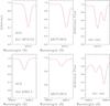 |
Fig. 1 Lines of Zn i fit to the solar spectrum observed with the UVES spectrograph and to spectra of Arcturus (Hinkle et al. 2000), and μ Leo observed with the ESPaDOns/CFHT spectrograph. Observed spectrum (dashed lines); synthetic spectra (solid red line). |
Zinc lines were checked against oscillator strengths log gf in the literature, using in particular the data bases from Kurúcz (1995) website2, NIST3, and VALD (Piskunov et al. 1995). Table 1 reports excitation potential, log gf values from the literature with their references, and adopted log gf values. The lines were fitted to the solar high resolution observations using the same UVES spectrograph4 as the present sample of spectra, to spectra from Arcturus (Hinkle et al. 2000), and from the metal-rich giant μ Leo, with spectra observed with the ESPaDOns/CFHT spectrograph, at a resolution of R ~ 80 000 and a signal-to-noise ratio of S/N ~ 500 (Lecureur et al. 2007). The fits of Zn i 4810.529 and 6362.339 Å lines in these reference stars are presented in Fig. 1.
2.1. Autoionization of Ca i lines
The measurement of the Zn i 6362.350 line has to take a continuum lowering in the range ~6360.8−6363.1 Å into account, owing to the Ca i 6361.940 auto-ionization line. Mitchell & Mohler (1965) identified depressions that are ~2.6 Å wide at the locations of the Ca i multiplet lines at 6318, 6343, and 6363 Å, which are caused by auto-ionizing transitions 3d4p 3F°−3d4d 3G. Following the recipe that Lecureur et al. (2007) used for the 6318 Å line, we adjusted the radiative broadening factor for the 6363 Å line to match the line profile to standard stars (Sun, Arcturus, μ Leo), as well as to sample stars, thus taking the much reduced lifetime of the level suffering auto-ionization into account. The best-fitting value is 32 000 higher than the standard radiative broadening (γrad = 0.21 /λ2). Taking this effect into account, we derived an astrophysical log gf value for the Ca i 6361.940 line, as reported in Table 1.
2.2. Solar abundances
Table 2 gives literature abundances for Fe and Zn for the Sun, Arcturus, and μ Leo. The adopted solar abundances for Fe and Zn are from Grevesse & Sauval (1998), whereas for Arcturus they are from the present fits, when adopting stellar parameters from Meléndez et al. (2003). For the metal-rich star μ Leo, the stellar parameters and C, N, O abundances from Lecureur et al. (2007) were adopted: Teff = 4540 K, log g = 2.3, [Fe/H] = +0.3, vt = 1.3 km s-1. The C, N, O abundances for μ Leo were revised from ϵ(C) = 8.85, ϵ(N) = 8.55, ϵ(O) = 9.12, to [C/Fe] = −0.3, [N/Fe] = + 0.6, [O/Fe] = −0.1 or ϵ(C) = 8.55, ϵ(N) = 8.83, ϵ(O) = 8.97. Also for better fitting the line on the red side of the Zn i 4810.5 Å line, which is not well fitted with literature log gf values, we refitted them with the astrophysical log gf values reported in Table 1, assuming [Cr/Fe] = [Ti/Fe] = 0.0 for μ Leo. Finally, for μ Leo, the resulting Zn abundance of [Zn/Fe] = −0.1 is derived from both ZnI lines.
Adopted abundances for the Sun, Arcturus, and μ Leo.
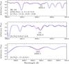 |
Fig. 2 CNO in B6-b6: fits to the Swan C2 (0, 1) bandhead at 5635.2 Å, the red CN (5, 1) bandhead at 6332.18 Å, and the forbidden oxygen [OI]6300.31 Å line. Dotted line: observed spectrum; red line: synthetic spectra giving the best fit: [C/Fe] = −0.07, [N/Fe] = +0.7, [O/Fe] = 0.0; blue lines: synthetic spectra computed with [C/Fe] = −0.10 and −0.05, [N/Fe] = +0.6 and +0.8, and [O/Fe] = −0.1 and +0.1. |
3. Abundance analysis
Elemental abundances were obtained through line-by-line spectrum synthesis calculations, carried out using the code described in Barbuy et al. (2003) and Coelho et al. (2005). The molecular lines present in the region, namely the CN B2Σ-X2Σ blue system, CN A2Π-X2Σ red system, C2 Swan A3Π-X3Π, MgH A3Π-X3Σ+, and TiO A3Φ-X3Δγ and B3Π-X3Δγ’ systems were taken into account. The atmospheric models were obtained by interpolation in the grid of MARCS LTE models (Gustafsson et al. 2008). The stellar parameters, reported in Table 6, were adopted from the detailed analyses by Zoccali et al. (2006) and Lecureur et al. (2007) for 43 bulge field red giants. Another 13 field red clump stars were analysed by Hill et al. (2011) based on both the UVES and the GIRAFFE spectra. We adopted the parameters derived from the UVES spectra, which were not given in Hill et al. (2011) but already reported in Barbuy et al. (2013).
3.1. C, N, O abundances and blending CN lines
The Zn i 6362.339 Å line is blended with the CN lines reported in Table 3, corresponding to the laboratory measurements by Davis & Phillips (1963). We initially adopted the C, N, and O abundances derived in Lecureur et al. (2007). Based on the observed profile of the Zn i 6362 Å line, however, we realized that in some cases the CN blend was overestimated, producing a spurious asymmetry in the red wing of the Zn i 6362 Å line. In these cases (16 stars marked with ** in Table 6), we recomputed C, N, and O abundances. We finally decided to recompute C, N, and O for all sample stars, given the influence of the CN blend in the Zn abundance derivation from the Zn i 6362 Å line. Oxygen was also derived for the two most metal-poor stars of the sample BW-f4 and BW-f8, for which no previous derivation was available.
The derivation of C, N, and O abundances was carried out by fitting the Swan C2 (0,1) A3Π-X3Π bandhead at 5635 Å, the red CN (5,1) A2Π-X2Σ bandhead at 6332.18 Å, and the forbidden oxygen [OI]6300.311 Å line. Fits to these C,N,O abundance indicators are illustrated in Fig. 2 for star B6-b6. These features have to be fitted iteratively, given that a change in the abundance of any of them has an impact on the molecule dissociative equilibrium. A further check of the CN line intensity was done for the asymmetry of the Zn i 6362 Å line.
In Table 6 we report the Lecureur et al. (2007) C, N, O abundances, and in the next column, we assign the letter c when the abundance is confirmed; otherwise, we give the newly revised abundances. A few comments on individual stars are given in the last column of Table 6: Telluric means that such lines mask the [OI]6300 and [OI]6363 lines, thus preventing any possibility of deriving its oxygen abundance, such as in BL-7; by the comment “CN-strong”, we mean that CN lines that are too strong blend the Zn i 6362 Å line, leading to this line being discarded in 15 stars: B6-b2, B6-f1, B6-f8, BW-b5, BW-f1, BW-f7, B3-b3, B3-b5, B3-b7, B3-f5, BWc-2, BWc-3, BWc-5, BWc-6, and BWc-8.
No Zn lines were useful for stars B3-b3, B3-f5, and BWc-2, but they were kept in the line list for reporting their C, N, O abundance derivation. This means that we derived Zn abundances for 53 (and not 56) stars. In about a third of the sample stars, an asymmetry due to the CN lines was clear, permitting a confirmation of the CNO abundances derived, such as for the star B3-b1.
These corrected C, N, O abundances were adopted here for the purpose of the present paper, which is to correct the derivation of the Zn abundances. A more thorough discussion of these revised oxygen abundances will be deferred to elsewhere. The Zn abundances were recomputed for the stars where the CNO abundances were revised, taking into account the newly derived C, N, O abundances, given in Col. 11 of Table 6, and the final Zn abundances are reported in Col. 14.
For the fit of the Zn i 4810 Å line, we adopted a procedure of balancing the continua points at the pseudo-continuum regions 4808.25, 4811.55, and 4812.6, with more weight for the 4811.55 Å that appears to be a better defined continuum. For the Zn i 6362.34 Å line, with a few exceptions, the local continuum is affected by the depression due to the Ca i line and, despite it being considered in the calculations, some extra depression remains. We gave priority to the continuum in the region 6361.5−6362.1 Å on the blue side of the Zn line. Examples of fitting ZnI lines in sample spectra are given in Figs. 3−6 for stars B6-f1, B6-f8, BW-f8, and BWc-4. In these figures we also show the calculations with no Zn (synthetic spectra in blue), showing that the Zn i 4810 Å line is free of blends, and the Zn i 6362 Å line shows a blend with CN lines. These figures show examples of the cases of no interference by CN lines (BW-f8), a moderate or negligible presence of CN lines (BWc-4), and strong contaminating CN lines (B6-f1, B6-f8), leading us not to consider the line for such stars. Star B6-f8 shows a detectable good fit to the CN line on the red side of the Zn i 6362 Å line, but this indicator was discarded as well.
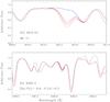 |
Fig. 3 Zn i 4810.54 and 6362.3 Å lines for star B6-f1. Dotted lines: observed spectra; red lines: synthetic spectra computed with the [Zn/Fe] values reported in the lower panels. The synthetic spectrum in blue has no Zn: for this star the Zn i 6362.3 Å line was discarded. |
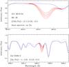 |
Fig. 4 Zn i 4810.54 and 6362.3 Å lines for star B6-f8. Dotted red and blue lines: same as in Fig. 3. The Zn i 6362.3 Å line was discarded for this star. |
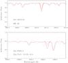 |
Fig. 5 Zn i 4810.54 and 6362.3 Å lines for star BW-f8. Dotted red and blue lines: same as in Fig. 3. |
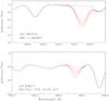 |
Fig. 6 Zn i 4810.54 and 6362.3 Å lines for red clump star BWc-4. Dotted red and blue lines: same as in Fig. 3. |
As regards non-LTE corrections, Takeda et al. (2005) have computed non-LTE effects on both the Zn i 4810 and 6362 Å lines used here. The corrections are below 0.1 dex for the metal-poor stars and below 0.05 for stars with [Fe/H] > −1.0. Consequently, in the present work, we do not correct the abundances for this effect.
3.2. Errors
We have adopted uncertainties in the atmospheric parameters of ±150 K for effective temperature, ±0.20 for surface gravity, and ±0.10 in [Fe/H] and ±0.10 km s-1 for microturbulent velocity, as explained in Barbuy et al. (2013).
The errors in [Zn/Fe] are computed by using model atmospheres with parameters changed by these uncertainties, applied to the stars B6-f1 and BW-f8. The errors are estimated from the differences in [Zn/Fe], derived using the modified models relative to the adopted model. We adopt a mean of the uncertainty on the Zn i 4810 and 6362 Å lines. These uncertainties are given in Table 4 for star B6-f1, for which the Zn i 6362 line is strongly affected by the CN blending, and BW-f8 with negligible CN blending. The higher sensitivity to effective temperature in B6-f1 is due to the CN lines blending the Zn i 6362.339 Å line: it is the CN lines that are more sensitive to temperature. Since the stellar parameters are covariant, the sum of these errors is an upper limit. On the other hand, a continuum location uncertainty introduces a further uncertainty in [Zn/Fe] of ±0.1.
Uncertainties on the derived [Zn/Fe] value for model changes of ΔTeff = +150 K, Δlog g = + 0.2, Δ[Fe/H] = +0.1 dex, Δvt = + 0.1 km s-1, and corresponding total error.
4. Results
The derived Zn abundances are given in Table 6. In Fig. 7, the [Zn/Fe] vs. [Fe/H] behaviour is shown for the present sample, where different symbols represent the four different fields, and the red clump stars. In Fig. 7a, we overplotted the Zn abundances of dwarf bulge stars observed thanks to microlensing magnification, by Bensby et al. (2013). There is good agreement between the present results and those by Bensby et al. at metallicities −1.4 < [Fe/H] < 0.0. On the other hand, for our metal-rich giants with [Fe/H] > 0.0, we find a wide spread of −0.6 < [Zn/Fe] < + 0.15 and a decreasing trend with metallicity. Further comments on the Bensby et al. sample of dwarf bulge stars are given in Sect. 4.3. In Fig. 7b we show the same stars as in Fig. 7a, adding metal-poor halo stars analysed by Cayrel et al. (2004) and halo and thick disk stars results from Ishigaki et al. (2013) and Nissen & Schuster (2011). Ishigaki et al. results seem to show lower [Zn/Fe] in the −3.0 < [Fe/H] < −1.0 metallicity range with respect to the Nissen & Schuster and Cayrel et al. results.
4.1. Comparison with thick disk Zn abundances
In Fig. 8 we compare the present bulge Zn abundances with those for thick disk stars in the literature. The results by Nissen & Schuster (2011) are maintained in all panels in Fig. 8, showing good agreement with other samples of thick disk stars. Given the narrow spread and the metallicity range covered by these data, we adopted the Nissen & Schuster (2011) results as a reference for the thick disk. Panels a−d show the Zn abundances derived respectively by Bensby et al. (2014), Mishenina et al. (2011), Prochaska et al. (2000), and Reddy et al. (2006). All thick disk samples show very good agreement with the present data, in the metallicity range of thick disk stars (). The Bensby et al. (2014) thick disk stars were selected based on kinematical criteria TD/D> 2, with these numbers corresponding to a probability defined in Bensby et al. (2003). Thick disk stars from Bensby et al. (2014) displayed in Fig. 8a include an old metal-poor thick disk, whereas the more metal-rich thick disk stars are younger (<8 Gyr). The Bensby et al. old metal-poor thick disk stars, reaching down to [Fe/H] ≈ −2.0, show a moderate enhancement of [Zn/Fe] ≈ + 0.15, compatible with our results for the metal-poor bulge stars. Their more metal-rich thick disk component with [Fe/H] > −0.3 show Zn-to-iron essentially solar, whereas our sample includes stars with low Zn-to-iron. The metallicity limits for the thick disk often give [Fe/H] = −0.3 as an upper limit; however, Bensby et al. classify some of their more metal-rich stars as probable thick-disk members, based on kinematics, as explained above, and they tend to be younger than 8 Gyr. Comments on the Bensby et al. sample consisting of dwarfs are given below in Sect. 4.3.
In the metallicity range occupied by the old thick disk stars, the bulge appears compatible with the thick disk abundances for the samples from Bensby et al. (2014), Mishenina et al. (2011), Prochaska et al. (2000), and Reddy et al. (2006). A distinction between the present data and thick disk stars may be present for the metal-rich stars, where most stars in the present sample show Zn under-abundances, and the Bensby et al. data show [Zn/Fe] ~ 0.0. It is important to note that there are not as many such old metal-rich stars in the thick disk population studied by Bensby et al. (2013).
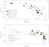 |
Fig. 7 [Zn/Fe] vs. [Fe/H] for present results compared with literature abundances for halo and bulge stars. Panel a): plotted in the metallicity range −1.5 < [Fe/H] < +0.7, corresponding to that of sample bulge giant stars, compared with the bulge dwarfs by Bensby et al. (2013). The subsamples are indicated by different symbols and identified by the central field (l, b) values; Panel b): plotted for −4.4 < [Fe/H] < + 0.7, encompassing halo stars from Cayrel et al. (2004), halo and thick disk stars from Ishigaki et al. (2013) and Nissen & Schuster (2011), and again the bulge dwarfs by Bensby et al. (2013). The symbols indicate: present data in black: open triangles: NGC 6553 field (designated B3), filled circles: Baade’s Window field (BW); open squares: field at −6° (designated B6); filled triangles: Blanco field (designated BL); open stars: Red clump stars in Baade’s Window (designated RC). Literature data: red three-pointed stars: Cayrel et al. (2004); green crosses: Ishigaki et al. (2013); red open circles: Nissen & Schuster (2011); green 3-pointed stars: Bensby et al. (2013). A representative error bar is given in the lower right corner of the upper panel. |
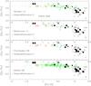 |
Fig. 8 [Zn/Fe] vs. [Fe/H] for present results (same symbols as in Fig. 7), compared with the thick disk analyzed by Nissen & Schuster (2011) (maintained in all panels in this figure), and the thick disk data by a) Bensby et al. (2014); b) Mishenina et al. (2011); c) Prochaska et al. (2000); d) Reddy et al. (2006). |
4.2. Comparison with thin disk Zn abundances
In Fig. 9 we compare the present Zn abundances with those for thin disk stars derived by Bensby et al. (2014), and Allende-Prieto et al. (2004). The data are also compared with the metal-rich dwarf stars from Pompéia (2003). Thick-disk stars by Nissen & Schuster (2011) are also kept in all plots, as a reference for the thick disk. The thin disk Zn abundances from Bensby et al. (2014) are consistent with a mean [Zn/Fe] ~ 0.0, with a fraction of stars showing higher [Zn/Fe] up to ~+0.4. The Allende-Prieto et al. (2004) stars show a mean [Zn/Fe] > 0 and an increasing trend with metallicity. The dwarf stars studied by Pompéia (2003) overlap with the present bulge stars data, except for the more metal-rich ones, which show no under-abundance. This difference may indicate that the Pompéia (2003) sample would be rather old thin disk stars and not bulge-like stars, as concluded in Trevisan et al. (2011) and again discussed in Trevisan & Barbuy (2014).
4.3. Inspecting differences with literature samples
The comparisons with literature data in the previous sections include several samples of dwarf stars: the microlensed dwarf bulge stars from Bensby et al. (2013), the thin and thick disk stars from Bensby et al. (2014), the thin disk stars from Allende-Prieto et al. (2004) and Pompéia (2003), and the halo and thick disk stars from Nissen & Schuster (2011). Bensby et al. (2013, 2014) and Allende-Prieto et al. (2004) used the Zn i 4810.5 and 6362.2 Å lines, and Nissen & Schuster (2011) used the Zn i 4722.1 and 4810.5 Å lines. (Pompéia 2003 does not report the lines used.)
The lines used are, in most cases, shared with the present work. The dwarfs are all hotter than the present sample, such that their samples have spectra with essentially no molecular lines. This could explain any difference in abundances from the Zn i 6362.2 Å line, that has a blend with CN lines affecting our determinations. On the other hand, the Zn i 4810.5 Å line has no molecular lines, and it shows the same Zn deficiencies as the Zn i 6362.2 Å line for many of the most metal-rich giant stars, but differently from the dwarfs.
The differences for metal-rich stars could stem from other blends, possibly unknown. At present we cannot identify a reason not to confirm the Zn-under-abundance in some of the present sample of metal-rich bulge giants. The flat or decreasing [Zn/Fe] at high metallicities has the important consequence of indicating (or not) the contribution of SNIa (see Sect. 4.5).
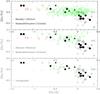 |
Fig. 9 [Zn/Fe] vs. [Fe/H] for present results compared with thin disk stars by a) Bensby et al. (2014); b) Allende-Prieto et al. (2004); c) Pompéia (2003). Thick disk stars by Nissen & Schuster (2011) are also shown in panels a) and b). |
4.4. Comparison with damped Lyman-α systems
A comparison of the present bulge data with DLAs is possible thanks to the availability of a large data base of Zn abundances over a wide range of metallicities for these objects. Such a comparison can shed light not only on the nature of DLAs, but also on the formation process of bulges.
The high H I column densities that characterize the DLAs indicate that they belong to environments with relatively high gas density, which could give rise to components of present day massive galaxies. The presence of metals in their spectra is also a clue that star formation has already taken place at significant rates inside them or in their neighbourhood. In this way, two favoured candidates for sites hosting DLAs are proto-disks and young star-forming spheroids. Lanfranchi and Friaça (2003) have investigated the evolution of the metallicity of DLAs in order to set constraints on the nature of these objects and also to shed light on the connections between DLAs and galaxy formation. The comparison of the observed trends of [α/Fe] and [N/α] with the predictions of a chemo-dynamical model is consistent with a scenario in which the DLA population is dominated by disks at low redshifts and by young spheroids at high redshifts. With the data base available for that work, nearly the totality of DLAs at z> 1.5 are explained as spheroid systems formed in the redshift range 1.7 <z< 4.5, with masses between 109 and 1010M⊙ and typical specific star formation rates of 1 to 3 Gyr-1, where the definition of specific star formation is given in the footnote below5. These objects might have taken part in merger processes that then lead to bulges. It is possible that the most massive of them, those with NHI ≈ 1022 cm-2, could be proto-bulges.
Zinc has played a special role in estimations of the metallicity of DLAs (Pettini et al. 1990, 1994, 1997a,b; Akerman et al. 2005). That Zn is non-refractory guarantees that it is not heavily depleted in the interstellar medium (ISM) . On the observational side, Zn has two strong transitions at 2026 and 2062 Å, which almost always lie outside the Ly-α forest and are rarely saturated owing to their low oscillator strengths and low Zn abundances. Given that Zn is only a trace element that contributes ≈ 10-4 of the mass density for the heavy elements, and because of the weakness of the Zn transitions, it is impossible to measure its abundance in low-metallicity DLAs, and besides that, the large rest-frame wavelengths of the transitions at 2026 and 2062 Å make them difficult to measure at high redshift.
Studies of Zn in damped Lyman-α systems with different redshifts have shown that [Zn/H] tends to show no correlation with distance and age. Akerman et al. (2005), for example, suggest that [Zn/H] in DLAs shows a constant value of [Zn/H] = −0.88 ± 0.21 in the redshift range 1.86 <zabs< 3.45. Comparisons of stellar data with abundances in DLAs were carried out by several authors (Pettini et al. 1994, 1997a; Prochaska et al. 2000; Wolfe et al. 2005; Nissen et al. 2007).
In Figs. 10a,b, we plot [Zn/H] vs. [Fe/H] for the present sample and for the DLA samples by Akerman et al. (2005), Cooke et al. (2011, 2013), Kulkarni et al. (2007), and Vladilo et al. (2011). For the Akerman et al. (2005) data, we did not consider the cases with upper limits alone. For the DLA samples of Kulkarni et al. (2007) and Vladilo et al. (2011), a tranformation [Fe/H] vs. redshift from the literature (Pei & Fall 1995) was adopted. Other such relations are given by Cen & Ostriker (1999) and Madau & Pozzetti (2000), for example. This figure shows that a comparison of Zn in DLAs and in bulge stars benefit from an overlap only at metallicities −1.5 < [Fe/H] < −0.1, with most sample bulge stars being more metal-rich than this.
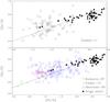 |
Fig. 10 [Zn/H] vs. [Fe/H] for the present sample (black filled triangles) and for the DLA samples by: (upper panel) Vladilo et al. (2011; open squares); (lower panel) Kulkarni et al. (2007; open squares), using a tranformation [Fe/H] vs. redshift from Pei & Fall (1995), and Cooke et al. (2013; green 3-pointed stars), Akerman et al. (2005; red four-pointed stars). A X = Y line is drawn. |
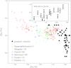 |
Fig. 11 [Zn/Fe] vs. [Fe/H] for the present sample and for the DLA samples by Akerman et al. (2005) and Cooke et al. (2013). We also plot the halo stars from Cayrel et al. (2004) and thick disk and halo stars data from Nissen & Schuster (2011) and Ishigaki et al. (2013). The inserted plot shows the trend for the dust depletion correction for the abundance of iron with the observed [Zn/H] derived from applying four distinct dust models to 16 DLAs. The curve is the quadratic fit to the trend that is used for dust correction. The abundances from the model calculations are averaged values inside several shells, shown as curves labelled according to the inner and the outer radius of each shell. |
4.4.1. Selected DLAs with Fe abundance measurements
For a few DLAs studied by Akerman et al. (2005) and Cooke et al. (2013), iron abundances ([Fe/H]) were measured, in addition to zinc abundances. We selected these objects to analyse the relation between the abundances of iron and zinc in DLAs. Vladilo et al. (2011) quote only [Zn/H] values for most of their DLA sample. However, they were able to derive, based on archive UVES spectra, the Fe ii column densities for two DLAs of their Zn ii + S ii sample , 0216+080 at zabs = 2.2930, and 2206-199A at zabs = 1.9200, which we also include in our list of measured Fe abundances in DLAs. An important concern is that Fe is a refractory element, and its depletion from the gas phase (observed through the absorption lines) into dust has to be taken into account. Therefore we applied a dust correction to the [Fe/H] values of the Akerman et al. (2005) and Vladilo et al. (2011) subsamples. No dust correction was needed for the Cooke et al. data, because their systems have [Fe/H] < −2, and at these low metallicities dust depletion becomes negligible (Pettini et al. 1997a). The systems for which we apply dust-depletion corrections for Fe are listed in Table 5.
DLA systems for which Fe abundances were measured, to which dust depletion corrections were applied.
Applying dust corrections to the chemical abundances of a gas system, either a DLA or the Galactic ISM, is a very complex task. We considered a variety of dust correction models, following Lanfranchi & Friaça (2003), to obtain the depletion δX of a given element X in the DLA, thus recovering the intrinsic abundance [X/H]i of that element from the observed one [X/H]: ![Mathematical equation: \begin{equation} \delta_{\rm X} \;=\; [{\rm X/H}] \; -\; [{\rm X/H}]_i . \end{equation}](/articles/aa/full_html/2015/08/aa25694-15/aa25694-15-eq106.png) (1)In the Galactic ISM, the suprasolar [Zn/Fe], [Zn/Cr], and [Zn/Si] ratios provide evidence of dust depletion by the refractories Fe, Cr, and Si. In addition, the dust depletion pattern depends on the type of environment through which the line of sight passes. Savage & Sembach (1996) considered four different dust depletion patterns corresponding to four types of Galactic ISM environments: (1) cool clouds in the Galactic disk (CD); (2) warm clouds in the disk (WD); (3) disk plus halo clouds (WHD); and (4) warm halo clouds (WH). On the other hand, we should consider a nucleosynthetic contribution to the Zn/Fe enhancement.
(1)In the Galactic ISM, the suprasolar [Zn/Fe], [Zn/Cr], and [Zn/Si] ratios provide evidence of dust depletion by the refractories Fe, Cr, and Si. In addition, the dust depletion pattern depends on the type of environment through which the line of sight passes. Savage & Sembach (1996) considered four different dust depletion patterns corresponding to four types of Galactic ISM environments: (1) cool clouds in the Galactic disk (CD); (2) warm clouds in the disk (WD); (3) disk plus halo clouds (WHD); and (4) warm halo clouds (WH). On the other hand, we should consider a nucleosynthetic contribution to the Zn/Fe enhancement.
In our dust corrections to the Fe abundances, we followed Lanfranchi & Friaça (2003). We applied four distinct dust models to 16 DLAs of Lanfranchi & Friaça (2003) with small uncertainties for the abundances of zinc, iron, and one more refractory element (Cr, Si, or Mg). We assumed a range for the intrinsic [Zn/Fe] ratio of 0.0 (solar), 0.1, 0.2, and 0.3. The suprasolar values of [Zn/Fe] are suggested by determinations of low metallicity objects and could be checked a posteriori. We take the WD and the WH as reference media. It is not appropriate to consider the cool clouds as a reference for the DLA environment, because the cool clouds exhibit levels of dust depletion ([Fe/Zn], [Cr/Zn], [Si/Zn]) that are much higher than those observed in DLAs, and the molecular hydrogen fractions are typically low in DLAs, in contrast to the large number of molecules in the cool clouds. In addition, by using models of chemical evolution, Vladilo et al. (2011) have shown that, for most of the DLAs in their sample, the iron depletion is within the range delimited by the values typical of WD and WH Galactic clouds.
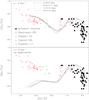 |
Fig. 12 Upper panel: comparison of the evolution of [Zn/Fe] with [Fe/H] in the stellar population predicted by a chemical evolution model for a classical bulge with star formation rate normalization νSF = 3 Gyr-1 and total mass of 1.5 × 10¹⁰M⊙, with the [Zn/Fe] vs. [Fe/H] data for the present sample, for the DLA samples by Cooke et al. (2013), Akerman et al. (2005) and Vladilo et al. (2011), and for the halo stars from Cayrel et al. (2004). The Fe abundances of Akerman et al. (2005) and Vladilo et al. (2011) have been corrected for dust depletion. (No dust correction was needed for the Cooke et al. sample, because their systems have [Fe/H] < −2.) Lower panel: the same as the upper model, but using, at low metallicities, the yields of Woosley & Weaver (1995) instead of those of hypernovae. |
The degree of depletion should increase with metallicity. We cannot use [Fe/H] directly to obtain the metallicity because iron itself is highly depleted into dust. Therefore, [Zn/H] is taken as a metallicity indicator because it is a volatile element. We derive a correction for dust depletion as a function of metallicity from the trend of the iron depletion predicted by the dust models with respect to the observed [Zn/H] values, applying the four distinct dust models to 16 DLAs. Then, a quadratic fit to the resulting total of 64 points gives the dust correction as a function of [Zn/H]. The inserted plot in Fig. 11 shows the trend of the dust depletion correction for the abundance of iron with the observed [Zn/H] derived from applying our dust models to the DLAs selected from Lanfranchi & Friaça (2003). The curve is the quadratic fit to the trend that is used for dust correction.
Finally, although less sensitive to dust depletion, the zinc abundance is also corrected in the way described in Lanfranchi & Friaça (2003). Figure 11 shows [Zn/Fe] vs. [Fe/H] for the DLA samples with determination of both [Zn/H] and [Fe/H], compared with the present results for bulge stars, thick disk, and halo stars from Nissen & Schuster (2011) and Ishigaki et al. (2011) and for metal-poor halo stars from Cayrel et al. (2004). The Akerman et al. (2005) and Vladilo et al. (2011) data have been corrected for dust depletion as explained above.
The Zn vs. Fe enrichment indicated by the DLA data from Akerman et al. (2005) and Vladilo et al. (2011) shows an overlap not only with thick disk and halo stars data from Nissen & Schuster (2011) and Ishigaki et al. (2013), but also with the pattern of the bulge stars, including a few subsolar [Zn/Fe] values.
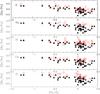 |
Fig. 13 [Zn/Fe] vs. [Fe/H] for the present sample (filled black triangles), compared with alpha-element abundances (open red squares), for oxygen, magnesium, silicon, calcium, and titanium. For oxygen all values are the presently revised oxygen abundances. |
4.5. Chemical evolution models of zinc in massive spheroids
Since bulge stars are probes of bulge formation and evolution, Fig. 12 shows the comparison of the [Zn/Fe] vs. [Fe/H] in bulge stars as derived in the present paper with a chemo-dynamical model describing a classical bulge. The computed models assume a specific star formation rate of νSF = 3 Gyr-1, a baryonic mass of 2 × 10⁹M⊙, and a dark halo mass MH = 1.3 × 10¹⁰M⊙ (total mass of 1.5 × 10¹⁰M⊙, thus reproducing the cosmological proportion of baryonic mass, Ωb = 0.04, to total matter mass, Ωm = 0.3). In the present calculations, we adopt an Ωm = 0.3, ΩΛ = 0.7, H0 = 70 km s-1 Mpc-1 cosmology, with the corresponding age of the universe of 13.47 Gyr. (An age of 13.799 ± 0.038 Gyr is the most recent and updated value from the Planck satellite data as given by the Planck collaboration I 2015).
The evolution of the model is followed until 13 Gyr, and it gives the evolution of the average Zn chemical abundance of the stellar population for several radii. As can be seen in Fig. 12, its end point falls in the locus of the data for the present-day stars in the bulge of the galaxy. The trend towards decreasing [Zn/Fe] ratio with increasing [Fe/H] for higher metallicities is reproduced well by the model. This is because although the bulge is formed rapidly in the classical scenario, the star formation goes on for a few Gyr. In the present case, the stellar mass is built up during at least ≈ 3 Gyr, which allows the contribution of type Ia SNe (SNIa) to be relevant, increasing the Fe abundance. The ejecta of SNIa exhibit a very low [Zn/Fe] ratio. The present model uses the SNIa yields of Iwamoto et al (1999), [Zn/Fe] ≈ −1.2 for a zero initial metallicity, and [Zn/Fe] ≈−1.6 for a solar initial metallicity. Therefore, as a result of the continuing star formation, the classical bulge model predicts subsolar [Zn/Fe] ratios for higher metallicities, as observed in the present sample of bulge stars.
The nucleosynthetic nature of Zn is complex; it is neither an α-element nor a Fe peak element. Theoretical work on the nucleosynthesis of Zn often predicts that it may originate in massive stars, but a complete network for production of Zn is not yet available. For instance, the classical core-collapse SN II yield calculations of Woosley & Weaver (1995) are known to underestimate the Zn abundance. One solution to this problem could be α-rich freeze-out neutrino winds, as predicted by Woosley & Hoffman (1992). On the other hand, Umeda & Nomoto (2002) have produced nucleosynthesis calculations in core-collapse explosions of massive low metallicity stars that do show large [Zn/Fe] for deeper mass cuts, smaller neutron excesses, and higher explosion energies. In the last case, the SN would be classified as a hypernova as defined by Nomoto et al. (2013, and references therein). Therefore, in the nucleosynthesis input of our chemical calculations, we consider the core-collapse SN II models of Woosley and Weaver (1995), but, for lower metallicities, we use the results of high explosion-energy hypernovae (Umeda & Nomoto 2002, 2003, 2005; Nomoto et al. 2006; 2013).
In summary, most of the bulge star data obtained in this work can be explained by a classical scenario of bulge formation. The trend towards a decreasing [Zn/Fe] ratio with increasing [Fe/H] seems to be reproduced well by the model. In addition, the model also accounts for the abundances of the halo stars, which can be thought of as a relic of the same galaxy formation sequence of events that gave rise to the bulge. The high [Zn/Fe] ratio of our calculations results from including hypernovae. The sensitivity of our results to the nucleosynthesis prescription is shown in the lower panel of 12, in which the Woosley & Weaver (1995) yields are used at low metallicities. The resulting [Zn/Fe] is very low, which favours hypernovae at low metallicities, as given in the upper panel. Finally, the decreasing trend of [Zn/Fe] at high metallicities is due to Fe enrichment from SNIa.
4.6. Zn and alpha elements
The Zn enhancement in metal-poor stars suggests that [Zn/Fe] behaves like alpha elements. For this reason, in Fig. 13 we compare the Zn abundances with those for the alpha elements O, Mg, Si, Ca, and Ti, derived in Lecureur et al. (2007), Zoccali et al. (2006), and Gonzalez et al. (2011). For oxygen the revised values given in Table 6 for selected stars are plotted instead of the previous values. The trend shown by Zn appears similar to that of the alpha elements and, more strikingly, of oxygen and calcium. The low [Zn/Fe] for high metallicity stars is compatible with the oxygen abundances.
The variation in Zn in lockstep with alpha elements is made evident further in Fig. 14, where [Zn/O] shows essentially no trend with [Fe/H] or with [O/H].
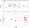 |
Fig. 14 [Zn/O] vs. [Fe/H] and [Zn/O] vs. [O/H] for the present sample, where the oxygen abundances are the revised ones from Table 6, otherwise those from Zoccali et al. (2006) and Lecureur et al. (2007). |
5. Conclusions
The iron-peak elements Sc, Mn, Cu, and Zn show a different chemical enrichment pattern than do the even-Z iron-peak elements Fe and Ni. In Barbuy et al. (2013), we confirmed that Mn behaves as a secondary element with low [Mn/Fe] in metal-poor stars, by increasing with increasing metallicity. In the present work we show that, in the metal-rich bulge stars, Zn-to-Fe decreases with increasing metallicity, complementing the long established high Zn abundances in metal-poor stars (e.g. Sneden et al. 1991; Nissen & Schuster 2011).
Our main comments on the comparison between the data points and models are the following: a) The most metal-rich bulge dwarfs from Bensby et al. (2013) show a constant [Zn/Fe], which implies that there is no contribution of SNe type I in the bulge, whereas a decrease in [Zn/Fe] in the present sample of giants, as derived here, implies that there is enrichment from Type I SNe as predicted by the models. The bulge stars are a complex mix of stellar populations of different ages and formation processes. b) The high [Zn/Fe] in very metal-poor stars favours enrichment from hypernovae, as defined by Nomoto et al. (2013 and references therein) acting at these low metallicities. It is interesting to point out that the hypernovae as defined by Nomoto et al. (2013) might be related to the spinstars as defined by Frischknecht et al. (2012) and Meynet et al. (2006) and discussed in terms of early enrichment of the bulge in Chiappini et al. (2011). c) The drop in [Zn/Fe] for moderately metal-poor stars () corresponds to the normal metal-poor SNe, here using the yields from Woosley & Weaver (1995).
For the DLA systems with measured Fe abundances, it was crucial to correct for dust depletion. The Zn abundances were also corrected for dust depletion, even if these corrections are smaller. The chemical evolution models predict subsolar [Zn/Fe] values at relatively high metallicities (), as confirmed for a few systems.
Online material
We adopted here the usual spectroscopic notation that [A/B] = log(NA/NB)⋆− log(NA/NB)⊙ and ϵ(A) = log(NA/NB) + 12 for the elements A and B.
Specific star formation rate (sSFR; in Gyr-1) is the ratio of the SFR in M⊙ Gyr-1 over the gas mass in M⊙ available for star formation.
Acknowledgments
B.B. acknowledges partial financial support by CNPq, CAPES, and FAPESP. C.R.S. acknowledges a CAPES/PROEX Ph.D. fellowship. M.Z. and D.M. acknowledge support by the Ministry of Economy, Development, and Tourism’s Millenium Science Initiative through grant IC120009, awarded to The Millenium Institute of Astrophysics, MAS, and from the BASAL Center for Astrophysics and Associated Technologies PFB-06 and FONDECYT Projects 1130196 and 1150345. S.O. acknowledges the Italian Ministero dell’Università e della Ricerca Scientifica e Tecnologica (MURST), Italy.
References
- Akerman, C. J., Ellison, S. L., Pettini, M., & Steidel, C. C. 2005, A&A, 440, 499 [NASA ADS] [CrossRef] [EDP Sciences] [Google Scholar]
- Allen de Prieto, C., Barklem, P. S., Lambert, D. L., & Cunha, K. 2004, A&A, 420, 183 [NASA ADS] [CrossRef] [EDP Sciences] [Google Scholar]
- Anders, E., & Grevesse, N. 1989, Geochim. Cosmochim. Acta, 53, 197 [Google Scholar]
- Asplund, M., Grevesse, N., Sauval, A. J., & Scott, P. 2009, ARA&A, 47, 481 [NASA ADS] [CrossRef] [Google Scholar]
- Barbuy, B., Perrin, M.-N., Katz, D., et al. 2003, A&A, 404, 661 [NASA ADS] [CrossRef] [EDP Sciences] [Google Scholar]
- Barbuy, B., Hill, V., Zoccali, M., et al. 2013, A&A, 559, A5 [NASA ADS] [CrossRef] [EDP Sciences] [Google Scholar]
- Bensby, T., Feltzing, S., & Lundström, I. 2003, A&A, 410, 527 [NASA ADS] [CrossRef] [EDP Sciences] [Google Scholar]
- Bensby, T., Yee, J. C., Feltzing, S., et al. 2013, A&A, 549, A147 [NASA ADS] [CrossRef] [EDP Sciences] [Google Scholar]
- Bensby, T., Feltzing, S., & Oey, M. S. 2014, A&A, 562, A71 [NASA ADS] [CrossRef] [EDP Sciences] [Google Scholar]
- Biémont, E., & Godefroid, M. 1980, A&A, 84, 361 [NASA ADS] [Google Scholar]
- Bisterzo, S., Gallino, R., Pignatari, M., et al. 2004, Mem. S. A.It. 75, 741 [Google Scholar]
- Cayrel, R., Depagne, E., Spite, M., et al. 2004, A&A, 416, 1117 [NASA ADS] [CrossRef] [EDP Sciences] [Google Scholar]
- Cen, R., & Ostriker, J. P. 1999, ApJ, 519, L109 [NASA ADS] [CrossRef] [Google Scholar]
- Chiappini, C., Frischknecht, U., Meynet, G., et al. 2011, Nature, 472, 454 [NASA ADS] [CrossRef] [Google Scholar]
- Coelho, P., Barbuy, B., Meléndez, J., Schiavon, R. P., & Castilho, B. V. 2005, A&A, 443, 735 [NASA ADS] [CrossRef] [EDP Sciences] [Google Scholar]
- Cooke, R., Pettini, M., Steidel, C. C., Rudie, G. C., & Nissen, P. E. 2011, MNRAS, 417, 1534 [NASA ADS] [CrossRef] [Google Scholar]
- Cooke, R., Pettini, M., Jorgenson, R. A., et al. 2013, MNRAS, 431, 1625 [NASA ADS] [CrossRef] [Google Scholar]
- Davis, S. P., & Phillips, J. G. 1963, The Red System (A2Π-X2Σ) of the CN molecule (Berkely: University of California Press) [Google Scholar]
- Gonzalez, O. A., Rejkuba, M., Zoccali, M., et al. 2011, A&A, 530, A54 [NASA ADS] [CrossRef] [EDP Sciences] [Google Scholar]
- Grevesse, N., & Sauval, J. N. 1998, SSRev, 35, 161 [Google Scholar]
- Gustafsson, B., Edvardsson, B., Eriksson, K., et al. 2008, A&A, 486, 951 [NASA ADS] [CrossRef] [EDP Sciences] [Google Scholar]
- Frischknecht, U., Hirschi, R., & Thielemann, F.-K. 2012, A&A, 538, L2 [NASA ADS] [CrossRef] [EDP Sciences] [Google Scholar]
- Hill, V., Lecureur, A., Gómez, A., et al. 2011, A&A, 534, A80 [NASA ADS] [CrossRef] [EDP Sciences] [Google Scholar]
- Hinkle, K., Wallace, L., Valenti, J., & Harmer, D. 2000, Visible and Near Infrared Atlas of the Arcturus Spectrum 3727–9300 A, eds. K. Hinkle, L. Wallace, J. Valenti, & D. Harmer (San Francisco: ASP) [Google Scholar]
- Ishigaki, M. N., Aoki, W., & Chiba, M. 2013, ApJ, 771, 67 [NASA ADS] [CrossRef] [Google Scholar]
- Iwamoto, K., Brachwitz, F., Nomoto, K., et al. 1999, ApJS, 125, 439 [NASA ADS] [CrossRef] [MathSciNet] [Google Scholar]
- Kobayashi, C., Umeda, H., Nomoto, K., Tominaga, N., & Ohkubo, T. 2006, ApJ, 643, 1145 [NASA ADS] [CrossRef] [Google Scholar]
- Kulkarni, V. P., Khare, P., Péroux, C., et al. 2007, ApJ, 661, 88 [NASA ADS] [CrossRef] [Google Scholar]
- Kurúcz, R. 1995, Atomic Line Data (R. L. Kurucz and B. Bell) Kurucz CD-ROM No. 23. Cambridge, Mass.: Smithsonian Astrophysical Observatory [Google Scholar]
- Lanfranchi, G., & Friaça, A. 2003, MNRAS, 343, 481 [NASA ADS] [CrossRef] [Google Scholar]
- Lecureur, A., Hill, V., Zoccali, M., Barbuy, B., et al. 2007, A&A, 465, 799 [NASA ADS] [CrossRef] [EDP Sciences] [Google Scholar]
- Lodders, K., Palme, H., & Gail, H.-P. 2009, Landolt-Börnstein – Group VI Astronomy and Astrophysics Numerical Data and Functional Relationships in Science and Technology Volume 4B: Solar System, ed. J. E. Trümper, 4.4, 44 [Google Scholar]
- Madau, P., & Pozzetti, L. 2000, MNRAS, 312, L9 [NASA ADS] [CrossRef] [Google Scholar]
- Meléndez, J., Barbuy, B., Bica, E., et al. 2003, A&A, 411, 417 [NASA ADS] [CrossRef] [EDP Sciences] [Google Scholar]
- Meynet, G., Ekström, S., & Maeder, A. 2006, A&A, 447, 623 [NASA ADS] [CrossRef] [EDP Sciences] [Google Scholar]
- Mishenina, T. V., Gorbaneva, T. I., Basak, N. Yu., et al. 2011, Astr. Rep., 55, 689 [NASA ADS] [CrossRef] [Google Scholar]
- Mitchell, W. E., & Mohler, O. C. 1965, ApJ, 141, 1126 [NASA ADS] [CrossRef] [Google Scholar]
- Nissen, P. E., & Schuster, W. J. 2011, A&A, 530, A15 [NASA ADS] [CrossRef] [EDP Sciences] [Google Scholar]
- Nissen, P. E., Chen, Y. Q., Schuster, W. J., & Zhao, G. 2000, A&A, 353, 722 [NASA ADS] [Google Scholar]
- Nissen, P. E., Akerman, C., Asplund, M., et al. 2007, A&A, 469, 319 [NASA ADS] [CrossRef] [EDP Sciences] [Google Scholar]
- Nomoto, K., Tominaga, N., Umeda, H., Kobayashi, C., & Maeda, K. 2006, Nucl. Phys. A, 777, 424 [NASA ADS] [CrossRef] [Google Scholar]
- Nomoto, K., Kobayashi, C., & Tominaga, N. 2013, ARA&A, 51, 457 [NASA ADS] [CrossRef] [Google Scholar]
- Pei, Y. C., & Fall, S. M. 1995, ApJ, 454, 69 [NASA ADS] [CrossRef] [Google Scholar]
- Pettini, M. 1990, Phil. Trans. R. Soc. Lond. A, 358, 2035 [NASA ADS] [CrossRef] [Google Scholar]
- Pettini, M., Smith, L. J., Hunstead, R. W., & King, D. L. 1994, ApJ, 426, 79 [NASA ADS] [CrossRef] [Google Scholar]
- Pettini, M., King, D. L., Smith, L. J., & Hunstead, R. W. 1997a, ApJ, 478, 536 [NASA ADS] [CrossRef] [Google Scholar]
- Pettini, M., Smith, L. J., King, D. L., & Hunstead, R. W. 1997b, ApJ, 486, 665 [NASA ADS] [CrossRef] [Google Scholar]
- Pettini, M., Ellison, S. L., Steidel, C. C., & Bowen, D. V. 1999, ApJ, 510, 576 [NASA ADS] [CrossRef] [Google Scholar]
- Piskunov, N., Kupka, F., Ryabchikova, T., Weiss, W., & Jeffery, C. 1995, A&AS, 112, 525 [NASA ADS] [Google Scholar]
- Planck collaboration I. 2015, A&A [arXiv:1502.01582] [Google Scholar]
- Pompéia, L. 2003, ApSSci, 299, 58 [Google Scholar]
- Prochaska, J. S., & Wolfe, A. M. 2002, ApJ, 566, 68 [NASA ADS] [CrossRef] [Google Scholar]
- Prochaska, J. S., Naumov, S. O., Carney, B. W., McWilliam, A., & Wolfe, A. M. 2000, AJ, 120, 2513 [NASA ADS] [CrossRef] [Google Scholar]
- Ramírez, I., & Allen de Prieto, C. 2011, ApJ, 743, 135 [NASA ADS] [CrossRef] [Google Scholar]
- Reddy, B. E., Lambert, D. L., & Allen de Prieto, C. 2006, MNRAS, 367, 1329 [NASA ADS] [CrossRef] [Google Scholar]
- Savage, B. D., & Sembach, K. R. 1996, ARA&A, 34, 279 [NASA ADS] [CrossRef] [Google Scholar]
- Sneden, C., Gratton, R. G., & Crocker, D. A. 1991, A&A, 246, 354 [NASA ADS] [Google Scholar]
- Takeda, Y., Hashimoto, O., Taguchi, H., et al. 2005, PASJ, 57, 751 [NASA ADS] [Google Scholar]
- Trevisan, M., & Barbuy, B. 2014, A&A, 570, A22 [NASA ADS] [CrossRef] [EDP Sciences] [Google Scholar]
- Trevisan, M., Barbuy, B., Eriksson, K., et al. 2011, A&A, 535, A42 [NASA ADS] [CrossRef] [EDP Sciences] [Google Scholar]
- Umeda, H., & Nomoto, K. 2002, ApJ, 565, 385 [NASA ADS] [CrossRef] [Google Scholar]
- Umeda, H., & Nomoto, K. 2003, Nature, 422, 871 [NASA ADS] [CrossRef] [PubMed] [Google Scholar]
- Umeda, H., & Nomoto, K. 2005, ApJ, 619, 427 [NASA ADS] [CrossRef] [Google Scholar]
- Vladilo, G., Abate, C., Yin, J., Cescutti, G., & Matteucci, F. 2011, A&A, 530, A33 [NASA ADS] [CrossRef] [EDP Sciences] [Google Scholar]
- Wolfe, A. M., Gawiser, E., & Prochaska, J. X. 2005, ARA&A, 43, 861 [NASA ADS] [CrossRef] [MathSciNet] [Google Scholar]
- Woosley, S. E., & Hoffman, R. D. 1992, ApJ, 395, 202 [NASA ADS] [CrossRef] [Google Scholar]
- Woosley, S. E., & Weaver, T. A. 1995, ApJS, 101, 181 [NASA ADS] [CrossRef] [Google Scholar]
- Zoccali, M., Lecureur, A., Barbuy, B., et al. 2006, A&A, 457, L1 [NASA ADS] [CrossRef] [EDP Sciences] [Google Scholar]
All Tables
Uncertainties on the derived [Zn/Fe] value for model changes of ΔTeff = +150 K, Δlog g = + 0.2, Δ[Fe/H] = +0.1 dex, Δvt = + 0.1 km s-1, and corresponding total error.
DLA systems for which Fe abundances were measured, to which dust depletion corrections were applied.
All Figures
|
Fig. 1 Lines of Zn i fit to the solar spectrum observed with the UVES spectrograph and to spectra of Arcturus (Hinkle et al. 2000), and μ Leo observed with the ESPaDOns/CFHT spectrograph. Observed spectrum (dashed lines); synthetic spectra (solid red line). |
| In the text | |
|
Fig. 2 CNO in B6-b6: fits to the Swan C2 (0, 1) bandhead at 5635.2 Å, the red CN (5, 1) bandhead at 6332.18 Å, and the forbidden oxygen [OI]6300.31 Å line. Dotted line: observed spectrum; red line: synthetic spectra giving the best fit: [C/Fe] = −0.07, [N/Fe] = +0.7, [O/Fe] = 0.0; blue lines: synthetic spectra computed with [C/Fe] = −0.10 and −0.05, [N/Fe] = +0.6 and +0.8, and [O/Fe] = −0.1 and +0.1. |
| In the text | |
|
Fig. 3 Zn i 4810.54 and 6362.3 Å lines for star B6-f1. Dotted lines: observed spectra; red lines: synthetic spectra computed with the [Zn/Fe] values reported in the lower panels. The synthetic spectrum in blue has no Zn: for this star the Zn i 6362.3 Å line was discarded. |
| In the text | |
|
Fig. 4 Zn i 4810.54 and 6362.3 Å lines for star B6-f8. Dotted red and blue lines: same as in Fig. 3. The Zn i 6362.3 Å line was discarded for this star. |
| In the text | |
|
Fig. 5 Zn i 4810.54 and 6362.3 Å lines for star BW-f8. Dotted red and blue lines: same as in Fig. 3. |
| In the text | |
|
Fig. 6 Zn i 4810.54 and 6362.3 Å lines for red clump star BWc-4. Dotted red and blue lines: same as in Fig. 3. |
| In the text | |
|
Fig. 7 [Zn/Fe] vs. [Fe/H] for present results compared with literature abundances for halo and bulge stars. Panel a): plotted in the metallicity range −1.5 < [Fe/H] < +0.7, corresponding to that of sample bulge giant stars, compared with the bulge dwarfs by Bensby et al. (2013). The subsamples are indicated by different symbols and identified by the central field (l, b) values; Panel b): plotted for −4.4 < [Fe/H] < + 0.7, encompassing halo stars from Cayrel et al. (2004), halo and thick disk stars from Ishigaki et al. (2013) and Nissen & Schuster (2011), and again the bulge dwarfs by Bensby et al. (2013). The symbols indicate: present data in black: open triangles: NGC 6553 field (designated B3), filled circles: Baade’s Window field (BW); open squares: field at −6° (designated B6); filled triangles: Blanco field (designated BL); open stars: Red clump stars in Baade’s Window (designated RC). Literature data: red three-pointed stars: Cayrel et al. (2004); green crosses: Ishigaki et al. (2013); red open circles: Nissen & Schuster (2011); green 3-pointed stars: Bensby et al. (2013). A representative error bar is given in the lower right corner of the upper panel. |
| In the text | |
|
Fig. 8 [Zn/Fe] vs. [Fe/H] for present results (same symbols as in Fig. 7), compared with the thick disk analyzed by Nissen & Schuster (2011) (maintained in all panels in this figure), and the thick disk data by a) Bensby et al. (2014); b) Mishenina et al. (2011); c) Prochaska et al. (2000); d) Reddy et al. (2006). |
| In the text | |
|
Fig. 9 [Zn/Fe] vs. [Fe/H] for present results compared with thin disk stars by a) Bensby et al. (2014); b) Allende-Prieto et al. (2004); c) Pompéia (2003). Thick disk stars by Nissen & Schuster (2011) are also shown in panels a) and b). |
| In the text | |
|
Fig. 10 [Zn/H] vs. [Fe/H] for the present sample (black filled triangles) and for the DLA samples by: (upper panel) Vladilo et al. (2011; open squares); (lower panel) Kulkarni et al. (2007; open squares), using a tranformation [Fe/H] vs. redshift from Pei & Fall (1995), and Cooke et al. (2013; green 3-pointed stars), Akerman et al. (2005; red four-pointed stars). A X = Y line is drawn. |
| In the text | |
|
Fig. 11 [Zn/Fe] vs. [Fe/H] for the present sample and for the DLA samples by Akerman et al. (2005) and Cooke et al. (2013). We also plot the halo stars from Cayrel et al. (2004) and thick disk and halo stars data from Nissen & Schuster (2011) and Ishigaki et al. (2013). The inserted plot shows the trend for the dust depletion correction for the abundance of iron with the observed [Zn/H] derived from applying four distinct dust models to 16 DLAs. The curve is the quadratic fit to the trend that is used for dust correction. The abundances from the model calculations are averaged values inside several shells, shown as curves labelled according to the inner and the outer radius of each shell. |
| In the text | |
|
Fig. 12 Upper panel: comparison of the evolution of [Zn/Fe] with [Fe/H] in the stellar population predicted by a chemical evolution model for a classical bulge with star formation rate normalization νSF = 3 Gyr-1 and total mass of 1.5 × 10¹⁰M⊙, with the [Zn/Fe] vs. [Fe/H] data for the present sample, for the DLA samples by Cooke et al. (2013), Akerman et al. (2005) and Vladilo et al. (2011), and for the halo stars from Cayrel et al. (2004). The Fe abundances of Akerman et al. (2005) and Vladilo et al. (2011) have been corrected for dust depletion. (No dust correction was needed for the Cooke et al. sample, because their systems have [Fe/H] < −2.) Lower panel: the same as the upper model, but using, at low metallicities, the yields of Woosley & Weaver (1995) instead of those of hypernovae. |
| In the text | |
|
Fig. 13 [Zn/Fe] vs. [Fe/H] for the present sample (filled black triangles), compared with alpha-element abundances (open red squares), for oxygen, magnesium, silicon, calcium, and titanium. For oxygen all values are the presently revised oxygen abundances. |
| In the text | |
|
Fig. 14 [Zn/O] vs. [Fe/H] and [Zn/O] vs. [O/H] for the present sample, where the oxygen abundances are the revised ones from Table 6, otherwise those from Zoccali et al. (2006) and Lecureur et al. (2007). |
| In the text | |
Current usage metrics show cumulative count of Article Views (full-text article views including HTML views, PDF and ePub downloads, according to the available data) and Abstracts Views on Vision4Press platform.
Data correspond to usage on the plateform after 2015. The current usage metrics is available 48-96 hours after online publication and is updated daily on week days.
Initial download of the metrics may take a while.