| Issue |
A&A
Volume 579, July 2015
|
|
|---|---|---|
| Article Number | A75 | |
| Number of page(s) | 6 | |
| Section | Catalogs and data | |
| DOI | https://doi.org/10.1051/0004-6361/201526253 | |
| Published online | 01 July 2015 | |
Research Note
Potsdam Wolf-Rayet model atmosphere grids for WN stars⋆
Institut für Physik und Astronomie, Universität Potsdam, Karl-Liebknecht-Str. 24/25, 14476 Potsdam, Germany
e-mail: htodt@astro.physik.uni-potsdam.de; wrh@astro.physik.uni-potsdam.de
Received: 2 April 2015
Accepted: 6 May 2015
We present new grids of Potsdam Wolf-Rayet (PoWR) model atmospheres for Wolf-Rayet stars of the nitrogen sequence (WN stars). The models have been calculated with the latest version of the PoWR stellar atmosphere code for spherical stellar winds. The WN model atmospheres include the non-LTE solutions of the statistical equations for complex model atoms, as well as the radiative transfer equation in the co-moving frame. Iron-line blanketing is treated with the help of the superlevel approach, while wind inhomogeneities are taken into account via optically thin clumps. Three of our model grids are appropriate for Galactic metallicity. The hydrogen mass fraction of these grids is 50%, 20%, and 0%, thus also covering the hydrogen-rich late-type WR stars that have been discovered in recent years. Three grids are adequate for LMC WN stars and have hydrogen fractions of 40%, 20%, and 0%. Recently, additional grids with SMC metallicity and with 60%, 40%, 20%, and 0% hydrogen have been added. We provide contour plots of the equivalent widths of spectral lines that are usually used for classification and diagnostics.
Key words: stars: evolution / stars: mass-loss / stars: winds, outflows / stars: Wolf-Rayet / stars: atmospheres / stars: massive
The full set of synthetic spectra and the spectral energy distributions are available online at http://www.astro.physik.uni-potsdam.de/PoWR.html
© ESO, 2015
1. Introduction
The spectra of Wolf-Rayet (WR) stars are characterized by bright and broad emission lines (Wolf & Rayet 1867). Such spectra are formed in a strong stellar wind. The large expansion velocity in the expanding stellar atmosphere broadens the lines, while their emission character is mainly due to strong deviations from local thermodynamical equilibrium (LTE). Modeling expanding stellar atmospheres in non-LTE is a formidable task. Adequate models, however, are a prerequisite for a quantitative spectral analysis of WR spectra. A few model atmosphere codes that can be applied to WR spectra have been developed in the last decades, e.g., cmfgen (Hillier 1987; Hillier & Miller 1998; Hillier & Lanz 2001), fastwind (Santolaya-Rey et al. 1997; Repolust et al. 2004; Puls et al. 2005), and the Potsdam Wolf-Rayet (PoWR) code (first results published in Hamann & Schmutz 1987).
These codes have been significantly improved over the years with features like microclumping and iron-line blanketing (Hillier & Miller 1999; Gräfener et al. 2002). Although such models became a standard tool for analyzing stellar wind spectra, their use was often restricted to a small set of prototypical stars owing to the limitations of computing power and calculation times. With the recent technical advances, these limits have been removed, enabling the calculation of whole grids of models. Model atmosphere grids calculated with the PoWR code have been published in the past for WN (Hamann & Gräfener 2004) and WC (Sander et al. 2012) stars (i.e. WR stars of the nitrogen and carbon sequence, respectively) with Galactic metallicity. In this note we present new grids for WN stars, including an updated and extended version of the WN grids from Hamann & Gräfener (2004), as well as additional grids with chemical compositions for the Large Magellanic Clound (LMC, see Hainich et al. 2014) and for the Small Magellanic Cloud (SMC Hainich et al. 2015).
In the next section we briefly describe the parameters that define a PoWR model, followed by Sect. 3 where we present the model grid parametrization. The synthetic spectra are introduced in Sect. 4. In Sect. 5 we give examples of the contour plots that can be used to find the best-fitting model to an observation. The models can also be used to obtain synthetic photometry and ionizing fluxes as shown in Sect. 6. Finally, in Sect. 7, we briefly describe the online interface that allows the model data described in this paper to be retrieved.
2. Model parameters
Our non-LTE model atmospheres are calculated with the PoWR code. Its basic assumptions are spherical symmetry and stationarity of the flow. The radiative transfer equation is solved in the comoving frame of the expanding atmosphere, iteratively with the equations of statistical equilibrium and radiative equilibrium. For more details on the PoWR code, see Hamann & Gräfener (2004).
The main parameters of a WR model atmosphere are the luminosity L and the stellar temperature T∗. The latter is the effective temperature related to the stellar radius R∗ via the Stefan-Boltzmann law  (1)The stellar radius R∗ is by definition located at a radial Rosseland continuum optical depth of 20, which represents the inner boundary of the model atmosphere.
Additional parameters that describe the stellar wind can be combined in the so-called transformed radius Rt. This quantity was introduced by Schmutz et al. (1989); we define it as  (2)with ν∞ denoting the terminal wind velocity, Ṁ the mass-loss rate, and D the clumping contrast (see below). Schmutz et al. (1989) noticed that model spectra with equal Rt have approximately the same emission line equivalent widths, independent of the specific combination of the particular wind parameters, as long as T∗ and the chemical composition are the same. Even the line profiles are conserved under the additional condition that v∞ is also the same. One can understand this invariance when realizing that Rt is related to the ratio between the volume emission measure and the stellar surface area.
According to this scaling invariance, a model can be scaled to a different luminosity as long as Rt and T∗ are unchanged. Equations (1) and (2) imply that the mass-loss rate must then be scaled as L3 / 4 in order to preserve the normalized line spectrum.
Allowing for wind inhomogeneities, the density contrast D is the factor by which the density in the clumps is enhanced compared to a homogeneous wind of the same Ṁ. We account for wind clumping in the approximation of optically thin structures (Hillier 1991; Hamann & Koesterke 1998). From the analysis of the electron-scattering line wings in Galactic WN stars, Hamann & Koesterke (1998) found that a density contrast of D = 4 is adequate. Crowther et al. (2010) and Doran et al. (2013) inferred D = 10 in their analyses of WN stars in the 30 Doradus region. For the LMC-WN models, we uniformly adopt a density contrast of D = 10 as in Hainich et al. (2014). We note that the empirical mass-loss rate derived from a given observed spectrum scales with the adopted density contrast D− 1 / 2 (cf. Eq. (2)).
For the Doppler velocity νD, describing the line broadening due to microturbulence and thermal motion, we adopt a value of 100 km s-1, which provides a good fit to observed line profiles (e.g., Hamann & Koesterke 2000; Hamann et al. 2006).
For the velocity law ν(r) in the supersonic part of the wind, we adopt the so-called β-law:  (3)For the exponent β, the radiation-driven wind theory predicts β ≈ 0.8, in agreement with observations of O star winds (e.g., Pauldrach et al. 1986). In WN stars, the law is shallower because of multiple-scattering effects. We adopt β = 1, which better resembles the hydrodynamic prediction (Gräfener & Hamann 2007) and yields consistent spectral fits. For the SMC grid models a double-β law (Hillier & Miller 1999) is used:
 ![\begin{eqnarray} v(r) = v_\infty \left[0.6\left(1-\frac{r_0}{r} \right) + 0.4\left(1 -\frac{r_1}{r} \right)^4 \right]\cdot \label{eq:doublebeta} \end{eqnarray}](/articles/aa/full_html/2015/07/aa26253-15/aa26253-15-eq23.png) (4)In the subsonic part, the velocity field is implied by the hydrostatic density stratification according to the continuity equation. The parameters r0 and r1 correspond roughly to the stellar radius R∗ and are adjusted such that the quasi-hydrostatic part and the wind are smoothly connected.
(4)In the subsonic part, the velocity field is implied by the hydrostatic density stratification according to the continuity equation. The parameters r0 and r1 correspond roughly to the stellar radius R∗ and are adjusted such that the quasi-hydrostatic part and the wind are smoothly connected.
The models are calculated using complex atomic data of H, He, C, and N. Iron group elements are considered in the “superlevel approach” that encompasses ~107 line transitions between ~105 levels within 72 superlevels (Gräfener et al. 2002).
3. The grids
The PoWR models published online are arranged in two-dimensional grids. All models in one grid have the same chemical composition and are calculated at the same terminal velocity. All models of these grids are calculated for a luminosity of log (L/L⊙) = 5.3. They can be scaled to different luminosities according to the scaling invariance discussed above (Sect. 2).
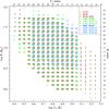 |
Fig. 1 Overview of Galactic, LMC, and SMC WN model grids in the log Rt–log T∗ plane. The different colors and symbols refer to the different grids described in Table 1. Each symbol represents a calculated PoWR model. |
The two free grid parameters are the stellar temperature T∗ and the transformed radius Rt. For convenience these two parameters are encoded in an index scheme reflecting the logarithmic steps. Each model has a label in the form k-m with the first index k encoding the temperature  (5)and the second index m encoding the transformed radius
  (6)While the index k increases with temperatures T∗, the second index m increases with decreasing values of Rt (cf. Fig. 1). The observed line-strength and the mass-loss rate Ṁ increase with higher values of index m (for a fixed k index). Within a grid, the mass-loss rate is constant along diagonals (k−m = const.) in the log Rt–log T∗ plane.
Wolf-Rayet stars are spectroscopically divided into the subclasses WN, WC, and WO (Kingsburgh et al. 1995; Crowther et al. 1998); WN stars predominantly show lines of helium and nitrogen, while WC and WO spectra exhibit strong emission lines of carbon and oxygen. The current paper deals only with WN-type stars.
The chemical composition of WN stars is mainly determined by two factors. The first is the metallicity of the host galaxy which defines the amount of the heavy elements of the star at formation.
For the Galaxy we adopt solar abundances of the iron group elements as given by Asplund et al. (2009). For the LMC and the SMC we scale these values by factors of 0.5 and 0.2, respectively (see discussion and references in Hainich et al. 2014, 2015).
While the initial amount of CNO also depends on the environment, the surface material of WN stars has already undergone partial CNO burning, as is evident from the depletion of hydrogen. As a consequence, almost all CNO material has been converted into nitrogen at the expense of carbon and oxygen. For the Galactic models, we assume a slightly supersolar amount of CNO material as found in the inner regions of the Milky Way where many WR stars reside. The nitrogen mass fraction is set to 1.5%, while carbon is depleted at 0.01%. Oxygen is not included in the models because it is depleted and without detectable lines in the spectra of typical WN stars. Correspondingly smaller values for the CNO abundances are adopted for the LMC and SMC (see discussion and references in Hainich et al. 2014, 2015).
The second factor that determines the chemical composition of WN winds is the amount of hydrogen. The hydrogen mass fraction can range from zero to ≈60% (e.g., Hamann et al. 2006; Sander et al. 2014). In the Galaxy and M 31, hydrogen-free WN stars are usually of early subtypes (WNE), while late subtype WN stars (WNL) typically show detectable hydrogen. We therefore abbreviate our hydrogen-free model grids as “WNE”, and those with hydrogen as “WNL” followed by, e.g., “-H50” for 50% H by mass.
As is evident from Rydberg’s formula, each spectral line of hydrogen is accompanied by the He ii line involving the doubled principle quantum numbers. In WR spectra, these neighboring lines are generally blended because of wind broadening. Therefore, a quantitative determination of the hydrogen abundance in WR stars requires detailed spectral modeling. For each of the metallicities considered, we provide a few grids with different hydrogen content.
Another free parameter of the models is the terminal wind velocity, v∞ (cf. Sect. 2). According to the scaling invariance discussed above, models that differ in v∞ show approximately the same emission line equivalent widths, as long as their Rt (cf. Eq. (2)) is the same. The line profiles, however, may differ owing to the wind broadening.
For each of the model grids, we chose a fixed value for v∞. Since WNE stars show typically faster winds than WNL stars, we adopt v∞ = 1600 km s-1 for the former and 1000 km s-1 for the latter.
Details of the grid parameters, abundances, and atomic data used in the models are given in Tables 1 and 2, respectively.
Model grid parameters.
Non-LTE levels for the WN model atmospheres.
4. Synthetic spectra
The synthetic line spectra are the most important output of the model simulations. They are calculated in the observer’s frame.
For each model, we provide synthetic spectra for the UV, optical, and infrared range. The spectra can be retrieved as continuum normalized or in absolute flux units. The wavelength resolution of the spectra corresponds to 0.3 vD, i.e., 30 km s-1 in velocity space.
An example of a normalized PoWR model spectrum can be seen in Fig. 2 where we demonstrate the effect of the different metallicities on the spectral appearance for a typical WN star.
5. The contour plots
In order to find the best-fitting model from a set of models to reproduce a particular observation, it is helpful to start by comparing the observed line strengths with those in the models. For convenience, we provide contour plots for each grid. For several diagnostic emission lines, contours of the same equivalent widths Wλ are shown in the log Rt–log T∗ plane. By comparing the measured value of Wλ in the observation with the contours in these plots, one can quickly identify the parameter regime that should give the best fit. Figure 3 shows the combined contours for the He i 5876 Å line and the He ii 5412 Å line from the Galactic WNL grid with XH = 0.2 as an example.
On the PoWR model website additional plots are available, including N iii 4640 Å, N v 4604-20 Å, C iv 5801-12 Å, and the infrared diagnostic line N iii 22500 Å.
Our models use the effective temperature T∗ as defined in Eq. (1), i.e., related to the radius where τRoss = 20. Other studies often use an effective temperature that refers to the radius where τRoss = 2/ 3, which we designate as  in the following. To illustrate how scales in our model grids, Fig. 4 shows contour lines of constant in the Galactic WNL model grid with XH = 0.2. The plot demonstrates that for denser winds (i.e., lower values of Rt), models with the same T∗ correspond to a lower . Such plots are provided for each model grid on the PoWR homepage.
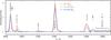 |
Fig. 2 Detail of the normalized spectra of hydrogen-free WN models with different metallicity with T∗ = 71 kK and Rt = 5.0 R⊙ (i.e., m-k = 10−14). The equivalent widths of the N and C lines decrease with decreasing metallicity, while the helium lines sta approximately unchanged. |
6. Spectral energy distribution for ionizing fluxes and photometry
The radiative transfer equation in the Non-LTE model atmospheres is calculated with up to 100 000 frequency points. For practical purposes, this fine frequency grid is later degraded to a coarse frequency grid of about 1/100th of the original resolution. The rebining is done such that the frequency integrals are conserved up to the first order. For the outermost radius of the model atmosphere, the emergent flux Fν is converted to fλ at 10 pc and made available as synthetic spectral energy distribution (SED) on the PoWR homepage. The synthetic SED can than be integrated over wavelength to obtain ionizing fluxes or convolved with a filter function to obtain photometric values, e.g., Johnson broadband magnitudes.
A warning must be issued regarding those parts of the SED where the fluxes are very small because of a strong absorption edge. The opacity at such wavelengths might be so large that the wind stays optically thick up to the outer boundary of our models. Hence, the corresponding emergent fluxes cannot be taken at face value (indicated by the gray shaded area in the example in Fig. 5).
This effect explains the apparent discrepancy of He ii ionizing fluxes between CMFGEN models (Smith et al. 2002) and PoWR models as reported by Pakull (2009). We calculated WN models with parameters as given in Table 3 in Smith et al. (2002) for 0.2 Z⊙ and 0.05 Z⊙ and found that their numbers of He ii ionizing photons for models with non-neglible He ii fluxes are comparable to ours. Discrepancies only occur for models, where the corresponding He ii ionizing flux is actually zero.
For convenience, we provide the number of the H i, He i, and He ii ionizing photons for every grid model on the PoWR website.
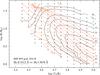 |
Fig. 3 Contour plots for He ii 5412 Å (thick blue lines) and He i 5876 Å (red dashed) in the WNL grid with XH = 0.2 and Galactic metallicity. |
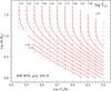 |
Fig. 4 Contour plot for |
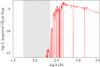 |
Fig. 5 Example of a spectral energy distribution from a WN model (red solid line), with log T∗/K = 4.8 and log Rt/R⊙ = 0.7 . The gray shaded area indicates the wavelength range of large opacity where the emergent flux is not reliable (see Sect. 6). |
7. Online interface
All mentioned model grids can be accessed online on our website1 with the emergent spectra both in normalized or flux-calibrated form, as well as the SED, available for direct download. As a first step, a model grid is selected out of the available WN/WC grids2. As a second step, the desired model can be selected by clicking on an interactive grid scheme. After selecting a model, one can choose to display additional information about the model parameters, such as Ṁ, M∗, or the stellar radius R∗. After confirming the selection one can choose between the SED and the normalized or flux-calibrated line spectrum. The additional button “colors” offers the monochromatic magnitudes at certain wavelengths and the number of ionizing photons. We note that the Smith photometry corresponds to monochromatic fluxes at wavelengths where usually no emission line is present. The button “stratification” prints out a table with depth dependent quantities such as densities, electron temperature, and velocity.
Finally, one can download the requested dataset or get a preview in either PostScript, PDF, or PNG format. If the line spectrum is selected, there will be an additional step included to choose the wavelength range. For all models, spectra are available in the UV, optical, and J, H, and K bands. Some models also contain the mid-IR (10 to 20 μm) regime, although we have not tested these spectra extensively for completeness and accuracy.
If you decide to use PoWR model spectra, please give references to this work and/or other papers depending on the type of model used. A list of references can also be found on the PoWR website. The PoWR code is applicable not only to WR stars,
but also to almost all hot stars with winds, including O and B stars (cf. Oskinova et al. 2011; Evans et al. 2012; Shenar et al. 2015; Sander et al. 2015) and low-mass stars (Todt et al. 2013; Reindl et al. 2014). Model grids for OB stars are in preparation and will be published online in the near future.
For comparison, the older WN grids from Hamann & Gräfener (2004) are also available. Some information about Rt and links to the contour plots mentioned in Sect. 5 are also available here.
Acknowledgments
A. Sander is supported by the Deutsche Forschungsgemeinschaft (DFG) under grant HA 1455/22. T. Shenar is grateful for financial support from the Leibniz Graduate School for Quantitative Spectroscopy in Astrophysics, a joint project of the Leibniz Institute for Astrophysics Potsdam (AIP) and the Institute of Physics and Astronomy of the University of Potsdam.
References
- Asplund, M., Grevesse, N., Sauval, A. J., & Scott, P. 2009, ARA&A, 47, 481 [NASA ADS] [CrossRef] [Google Scholar]
- Crowther, P. A., De Marco, O., & Barlow, M. J. 1998, MNRAS, 296, 367 [Google Scholar]
- Crowther, P. A., Schnurr, O., Hirschi, R., et al. 2010, MNRAS, 408, 731 [NASA ADS] [CrossRef] [Google Scholar]
- Doran, E. I., Crowther, P. A., de Koter, A., et al. 2013, A&A, 558, A134 [NASA ADS] [CrossRef] [EDP Sciences] [Google Scholar]
- Evans, C. J., Hainich, R., Oskinova, L. M., et al. 2012, ApJ, 753, 173 [NASA ADS] [CrossRef] [Google Scholar]
- Gräfener, G., & Hamann, W.-R. 2007, in Massive Stars in Interactive Binaries, eds. N. St.-Louis, & A. F. J. Moffat, ASP Conf. Ser., 367, 131 [Google Scholar]
- Gräfener, G., Koesterke, L., & Hamann, W. 2002, A&A, 387, 244 [NASA ADS] [CrossRef] [EDP Sciences] [Google Scholar]
- Hainich, R., Rühling, U., Todt, H., et al. 2014, A&A, 565, A27 [NASA ADS] [CrossRef] [EDP Sciences] [Google Scholar]
- Hainich, R., Pasemann, D., & Todt, H. 2015, A&A, submitted [Google Scholar]
- Hamann, W., & Gräfener, G. 2004, A&A, 427, 697 [NASA ADS] [CrossRef] [EDP Sciences] [Google Scholar]
- Hamann, W., & Koesterke, L. 1998, A&A, 335, 1003 [NASA ADS] [Google Scholar]
- Hamann, W., & Schmutz, W. 1987, A&A, 174, 173 [NASA ADS] [Google Scholar]
- Hamann, W., Gräfener, G., & Liermann, A. 2006, A&A, 457, 1015 [NASA ADS] [CrossRef] [EDP Sciences] [Google Scholar]
- Hamann, W.-R., & Koesterke, L. 2000, A&A, 360, 647 [NASA ADS] [Google Scholar]
- Hillier, D. J. 1987, ApJS, 63, 947 [NASA ADS] [CrossRef] [Google Scholar]
- Hillier, D. J. 1991, A&A, 247, 455 [NASA ADS] [Google Scholar]
- Hillier, D. J., & Lanz, T. 2001, in Spectroscopic Challenges of Photoionized Plasmas, eds. G. Ferland, & D. W. Savin, ASP Conf. Ser., 247, 343 [Google Scholar]
- Hillier, D. J., & Miller, D. L. 1998, ApJ, 496, 407 [NASA ADS] [CrossRef] [Google Scholar]
- Hillier, D. J., & Miller, D. L. 1999, ApJ, 519, 354 [NASA ADS] [CrossRef] [Google Scholar]
- Kingsburgh, R. L., Barlow, M. J., & Storey, P. J. 1995, A&A, 295, 75 [NASA ADS] [Google Scholar]
- Oskinova, L. M., Todt, H., Ignace, R., et al. 2011, MNRAS, 416, 1456 [NASA ADS] [CrossRef] [Google Scholar]
- Pakull, M. W. 2009, in IAU Symp. 256, eds. J. T. Van Loon & J. M. Oliveira, 437 [Google Scholar]
- Pauldrach, A., Puls, J., & Kudritzki, R. P. 1986, A&A, 164, 86 [NASA ADS] [Google Scholar]
- Puls, J., Urbaneja, M. A., Venero, R., et al. 2005, A&A, 435, 669 [NASA ADS] [CrossRef] [EDP Sciences] [Google Scholar]
- Reindl, N., Rauch, T., Werner, K., Kruk, J. W., & Todt, H. 2014, A&A, 566, A116 [NASA ADS] [CrossRef] [EDP Sciences] [Google Scholar]
- Repolust, T., Puls, J., & Herrero, A. 2004, A&A, 415, 349 [NASA ADS] [CrossRef] [EDP Sciences] [Google Scholar]
- Sander, A., Hamann, W.-R., & Todt, H. 2012, A&A, 540, A144 [NASA ADS] [CrossRef] [EDP Sciences] [Google Scholar]
- Sander, A., Todt, H., Hainich, R., & Hamann, W.-R. 2014, A&A, 563, A89 [NASA ADS] [CrossRef] [EDP Sciences] [Google Scholar]
- Sander, A., Shenar, T., Hainich, R., et al. 2015, A&A, 999, 777 [Google Scholar]
- Santolaya-Rey, A. E., Puls, J., & Herrero, A. 1997, A&A, 323, 488 [NASA ADS] [Google Scholar]
- Schmutz, W., Hamann, W., & Wessolowski, U. 1989, A&A, 210, 236 [NASA ADS] [Google Scholar]
- Shenar, T., Oskinova, L., Hamann, W., et al. 2015, ApJ, accepted [arXiv:1503.03476] [Google Scholar]
- Smith, L. J., Norris, R. P. F., & Crowther, P. A. 2002, MNRAS, 337, 1309 [NASA ADS] [CrossRef] [Google Scholar]
- Todt, H., Kniazev, A. Y., Gvaramadze, V. V., et al. 2013, MNRAS, 430, 2302 [NASA ADS] [CrossRef] [MathSciNet] [Google Scholar]
- Wolf, C., & Rayet, G. 1867, Comptes Rendus de l’Académie des Sciences, 65, 292 [Google Scholar]
All Tables
All Figures
|
Fig. 1 Overview of Galactic, LMC, and SMC WN model grids in the log Rt–log T∗ plane. The different colors and symbols refer to the different grids described in Table 1. Each symbol represents a calculated PoWR model. |
| In the text | |
|
Fig. 2 Detail of the normalized spectra of hydrogen-free WN models with different metallicity with T∗ = 71 kK and Rt = 5.0 R⊙ (i.e., m-k = 10−14). The equivalent widths of the N and C lines decrease with decreasing metallicity, while the helium lines sta approximately unchanged. |
| In the text | |
|
Fig. 3 Contour plots for He ii 5412 Å (thick blue lines) and He i 5876 Å (red dashed) in the WNL grid with XH = 0.2 and Galactic metallicity. |
| In the text | |
|
Fig. 4 Contour plot for |
| In the text | |
|
Fig. 5 Example of a spectral energy distribution from a WN model (red solid line), with log T∗/K = 4.8 and log Rt/R⊙ = 0.7 . The gray shaded area indicates the wavelength range of large opacity where the emergent flux is not reliable (see Sect. 6). |
| In the text | |
Current usage metrics show cumulative count of Article Views (full-text article views including HTML views, PDF and ePub downloads, according to the available data) and Abstracts Views on Vision4Press platform.
Data correspond to usage on the plateform after 2015. The current usage metrics is available 48-96 hours after online publication and is updated daily on week days.
Initial download of the metrics may take a while.