| Issue |
A&A
Volume 579, July 2015
|
|
|---|---|---|
| Article Number | A107 | |
| Number of page(s) | 8 | |
| Section | Numerical methods and codes | |
| DOI | https://doi.org/10.1051/0004-6361/201526240 | |
| Published online | 08 July 2015 | |
Theoretical impact of fast rotation on calibrating the surface brightness-color relation for early-type stars
1 Laboratoire Lagrange, UMR7293, UNS/CNRS/OCA, 06300 Nice, France
e-mail: This email address is being protected from spambots. You need JavaScript enabled to view it.
2 Laboratoire Dynamique Moléculaire et Matériaux Photoniques, UR11ES03, Université de Tunis/ESSTT, Tunisie
3 Departamento de Astronomía, Universidad de Concepción, 2204240 Casilla 160-C, Concepción, Chile
4 Warsaw University Observatory, AL. Ujazdowskie 4, 00-478 Warsaw, Poland
5 Millenium Institute of Astrophysics, Cassilla 306, Santiago 22, Chile
Received: 1 April 2015
Accepted: 18 May 2015
Abstract
Context. The eclipsing binary method for determining distance in the local group is based on the surface brightness-color relation (SBCR), and early-type stars are preferred targets because of their intrinsic brightness. However, this type of star exhibits wind, mass-loss, pulsation, and rotation, which may generate bias on the angular diameter determination. An accurate calibration of the SBCR relation thus requires careful analysis.
Aims. In this paper we aim to quantify the impact of stellar rotation on the SBCR when the calibration of the relation is based on interferometric measurements of angular diameters.
Methods. Six stars with V − K color indices ranging between –1 and 0.5 were modeled using the code for high angular resolution of rotating objects in nature (CHARRON) with various rotational velocities (0, 25, 50, 75, and 95% of the critical rotational velocity) and inclination (0, 25, 50, 75, and 90 degrees). All these models have their equatorial axis aligned in an east-west orientation in the sky. We then simulated interferometric observations of these theoretical stars using three representative sets of the CHARA baseline configurations. The simulated data were then interpreted as if the stars were non-rotating to determine an angular diameter and estimate the surface-brightness relation. The V − K color of the rotating star was calculated directly from the CHARRON code. This provides an estimate of the intrinsic dispersion of the SBCR relation when the rotation effects of flattening and gravity darkening are not considered in the analysis of interferometric data.
Results. We find a clear relation between the rotational velocity and (1) the shift in zero point (Δa0) of the SBCR (compared to the static relation) and (2) its dispersion (σ). When considering stars rotating at less than 50% of their critical velocity, Δa0 and σ have about 0.01 mag, while these quantities can reach 0.08 and 0.04 mag, respectively, when the rotation is larger than 75% of the critical velocity. Besides this, the inclination angle mostly has an impact on the V − K color: i< 50° (resp. i> 50°) makes the star redder (resp. bluer). When considering the 150 models, Δa0 and σ have 0.03 and 0.04 mag, respectively. These values are slightly but not significantly modified (about 0.03 and 0.01 mag in Δa0 and σ, respectively) when considering different CHARA configurations. Interestingly, these 150 models, regardless of the interferometric configuration, are consistent with the empirical SBCR, which is within its dispersion of 0.16 mag. In addition, if one only considers projected rotational velocity Vrotsini lower than 100 km s-1, then Δa0 and σ have 0.02 and 0.03 mag, respectively.
Conclusions. To calibrate the SBCR interferometrically at the 0.02 mag precision (or lower), one should consider (1) a baseline configuration covering all directions of the (u, v) plan; (2) a sample of stars with rotational velocity lower than 50% of their critical velocity or, alternatively, stars with Vrotsini lower than 100 km s-1; (3) homogeneous visible and infrared photometry precisely at the 0.02 mag level or lower.
Key words: techniques: interferometric / stars: distances / stars: rotation / instrumentation: interferometers / methods: numerical / stars: early-type
© ESO, 2015
1. Introduction
Detached eclipsing double-lined spectroscopic binaries offer a unique opportunity to measure the distance to nearby galaxies directly and very accurately (Graczyk et al. 2011; Wyrzykowski et al. 2003, 2004; Bonanos et al. 2006; Macri et al. 2001). The distance to an eclipsing binary (EB) follows from the combination of the radii of both components determined from spectro-photometric observations with their respective limb-darkened angular diameters derived from the surface brightness color relation (SBCR; Evans 1992, 1991; Paczynski & Stanek 1998; Bohm-Vitense 1985; Stanek & Garnavich 1998; Udalski 2000). By applying this technique to eight long-period eclipsing binaries in the LMC, consisting of G-K type giants, Pietrzyński et al. (2013) obtained a distance to the LMC with 2% precision.
It would be extremely interesting to apply this method to early-type eclipsing binaries (O, B, A), which are much brighter and thus easier to detect (Pietrzyński et al. 2009; Mochejska et al. 2001; Vilardell et al. 2006; Pawlak et al. 2013). The only limitation is currently the precision of the surface-brightness relation. Recently, Challouf et al. (2014b; hereafter Paper I) derived the SBCR (as a function of the V − K color) for the first time and with a precision of about 0.16 mag using interferometric measurements (Challouf et al. 2012, 2014a). However, to achieve 0.02 mag of precision on the SBCR (or 1% in terms of distance), one has to consider the stellar activity in early-type stars, such as wind, mass-loss, pulsation, and the rotation, which together represent the most important effect on the SBCR.
The surface brightness relation allows the angular diameter of a star to be estimated from its different magnitudes. The usual way to improve the relation is to obtain more direct measurements of angular diameters for a better determination of the empirical relation. The uncertainties in the SBCR stems from the photometry (about 0.03 mag), but also from the angular diameter determination.
One of the limitations in the angular diameter determination is the classical use of a uniform disk model. Indeed, in many cases, the stars are deformed by rotation and thus the determination is biased and generates an additional source of uncertainty in the SBCR calibration. Interpreting the interferometric measurements with a rotating model is possible in principle but requires a very large number of measures (e.g., van Belle et al. 2001; Peterson et al. 2006; Monnier et al. 2007; Zhao et al. 2009). A recent review with several references to interferometric measurements of fast rotators is given by van Belle (2012). Therefore it is not compatible with a survey program. Moreover, the definition of the SBCR relationship including the impact of fast rotation on the surface brightness is something that is very complex so clearly beyond the scope of this paper. We define criteria for the rotational velocity or the projected velocity V sin i to correctly select the stars considered for the calibration of SBCR (Challouf et al. 2015).
The purpose of this work is thus to quantify the impact of stellar rotation on the SBCR and to determine the corresponding intrinsic dispersion (in magnitude) we could expect. The paper is structured as follows. In Sect. 2, we present the CHARRON code and the six reference non-rotating models we consider. We then apply various values of rotation rates and inclination to these models, which gives us a sample of 150 models. In Sect. 3, we explain our methodology and show, in particular, how the V − K colors and the surface brightness are defined. To derive the surface brightness from the intensity distribution of a star, we simulated interferometric observations and proceed as if the star considered was not rotating. For one model, we show how the V − K color and the surface-brightness quantities are varying as a function of the rotational velocity and the inclination of the star. In Sect. 4 we present the derived SBCR relation and estimate its dispersion. We also clarify how this dispersion varies when considering different sets of stars with different rotational velocities. We discuss the implication of our results in the framework of Paper I in Sect 5.
2. CHARRON model for fast-rotating stars
The numerical model of fast-rotating star used here is the code CHARRON (code for high angular resolution of rotating objects in nature) described by Domiciano de Souza et al. (2012a,b, 2002). The stellar photospheric shape is given by the commonly adopted Roche approximation (rigid rotation and mass concentrated in the stellar center), which is well adapted to non-degenerate, fast-rotating stars.
The effective temperature Teff at the surface for fast rotators is not uniform (depending on the colatitude θ) owing to the decreasing effective gravity geff (gravitation plus centrifugal acceleration) from the poles to the equator (gravity darkening effect). We model the gravity darkening as a generalized form of the von Zeipel law (von Zeipel 1924):  (1)where β is the gravity darkening coefficient. von Zeipel (1924) derived a theoretical value of 0.25 for early-type stars with radiative external layers and pressure, only depending on the density (barotropic approximation). However, recent interferometric observations have measured somewhat lower values for β (e.g., Che et al. 2011; Domiciano de Souza et al. 2014).
The value of 0.20 seems a good compromise between the theoretical value of von Zeipel and most values measured from interferometric observations of fast-rotating stars and also with recent theoretical models of gravity darkening (e.g., Espinosa Lara & Rieutord 2011; Claret 2012). We thus consider β = 0.20 for our six models. The K is the proportionality constant between Teff and geff, which depends on the stellar physical parameters. Once Teff(θ) and geff(θ) are defined, we use the spectral synthesis code SYNSPEC (Hubeny & Lanz 2011) and the ATLAS9 stellar atmosphere models (Kurucz 1979) to compute the specific intensity maps of the star.
Parameters of the non-rotating models we use as a reference.
For this study of the SBCR relation, we define six reference models (non-rotating or static models) covering the range between –0.8 to 0.4 in terms of the V − K color index, which is typical of early-type stars. Using the online data from Worthey & Lee (2011), we find the effective temperature Teff and the surface gravity log g for each model, corresponding to a specific value of the V − K color. Using these quantities, we derive the corresponding mass and radius from Allende Prieto & Lambert (1999). The color index V − K, the effective temperature Teff, the surface gravity log g, the mass M, and the radius R are listed in Table 1. These parameters are used as input for the CHARRON code for the six non-rotating stars (M1 to M6). We then apply five values of the rotational velocity (0, 25, 50, 75, and 95% of the critical rotational velocity defined as the value of the rotation velocity at the equator such that the centrifugal acceleration compensates for the net radial attracting force, Vc in the following) and five values of the inclination angle of the rotation axis (0, 25, 50, 75, and 90 degrees). Zero (resp. 90) degrees corresponds to a pole-on (resp. edge-on) star.
3. The derived V – K color and surface brightness
In this section, we explain our methodology, including in particular how the V − K colors are derived from our 150 models and how we simulate interferometric observations in order to derive the calibration of the surface-brightness relation.
3.1. The V − K color
The stellar surface is divided into a predefined grid with nearly identical surface area elements (typically 50 000 surface elements). From Teff(θ) and geff(θ) defined in Domiciano de Souza et al. (2002), a local specific intensity from a plane-parallel atmosphere I = I(geff,Teff,λ) is associated with each surface element, where λ is the wavelength. (Limb darkening is thus automatically included in the model.) The stellar spectral flux in a solid angle dΩ is given by  (2)A surface-averaged Teff can be directly related to the flux fλ and to the mean angular diameter φ (diameter of spherical star having a surface area S) by
  (3)We defined the apparent magnitude mλ, which represents the flux of a star relative to a reference flux at a given wavelength,
  (4)The color index of our stars is defined as the difference between the apparent magnitude modeled in two different spectral bands,
  (5)We use the V and K bands, therefore mλ2 − mλ1 = V − K.
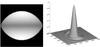 |
Fig. 1 Left: modeled intensity distributions; Right: the Fourier transform of the intensity map of M1 at 720 nm for 95% of Vc and i = 90°. |
3.2. From visibilities to surface brightness
3.2.1. The visibilities
The intensity distribution were derived from the CHARRON code for the 150 models we studied. An example is given in the left side of Fig. 1 in the case of M1. We then calculate the fast Fourier transform (FFT) of this intensity distribution following the theorem of Zernike-Van Cittert (van Cittert 1934; Zernike 1938), in which the interferometric visibility is defined as 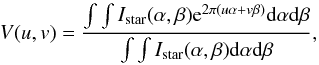 (6)where (α, β) are the angular coordinates in the plane of sky, while (u, v) are the spatial frequencies, defined as
  and
and  , with λ the wavelength of the incident radiation, Bu the u-component of the baseline vector B, Bv the v-component of the baseline vector B. Once the complex visibility is derived, we can determine the squared visibility, which provides the fringe contrast as a function of the spatial frequency (see Fig. 1-right) given by
 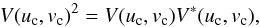 (7)where uc and vc are the spatial frequencies.
For our study we consider three realistic CHARA1 configurations indicated in Table 2. We decided to use the CHARA case because this interferometer presents the longest baselines and access to the visible wavelength, allowing thus to reach the best angular resolution and the one needed to accurately measure the considered stars. C1 and C2 are mainly oriented north-south and east-west, respectively, while C3 is a combination of C1 and C2 (Fig. 2). We mention here that our 150 models have their rotation axis aligned with the north-south direction.
CHARA configuration used in this study.
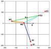 |
Fig. 2 Configuration of the CHARA array (ten Brummelaar et al. 2005) located at the Mount Wilson Observatory, north of Los Angeles (California, USA). The CHARA array consists of 6 telescopes of 1 meter in diameter, configured in a Y-shape, which offers 15 different baselines from 34 m to 331 m. |
3.2.2. The angular diameter
The squared visibilities (V2) obtained from the intensity distribution and the baseline configurations presented in the previous section are then interpreted using a simple uniform disk model. The theoretical visibility of this model is given by  where J1(z) is the Bessel function of the first kind and first order, and z = πθUDB/λ, where B is the projected baseline, λ the effective wavelength, and θUD the apparent UD angular diameter of the star.
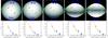 |
Fig. 3 Top: intensity maps are given in units of the equatorial radius (Req) with the project baselines in the sky. Bottom: squared visibility versus spatial frequency. The figures calculated for inclination (from left to right): 0°, 25°, 50°, 75°, and 90°. The rotational velocity for all inclinations is of 0.95Vc. The visibilities points presented with same color bases of Fig. 2, and the red lines are the best fitted uniform disk. The mean angular diameter θUD ranges from 0.635 ± 0.006 mas to 0.736 ± 0.001 mas. |
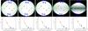 |
Fig. 4 Top: intensity maps given in units of the equatorial radius (Req) with the project baselines in the sky. Bottom: squared visibility versus spatial frequency. The figures calculated for rotational velocities (from left to right): 0.0Vc, 0.25Vc, 0.50Vc, 0.75Vc, and 0.95Vc. The inclination for all rotational velocities is 90°. The visibilities points presented with same color bases as in Fig. 2, and the red lines are the best-fitted uniform disk. The mean angular diameter θUD ranges from 0.635 ± 0.006 mas to 0.782 ± 0.001 mas. |
In Fig. 3, we present the squared visibility as a function of the spatial frequency in the case of the M1 model (Table 1) and the C3 configuration (Table 2). In the upper panel, the M1 model rotates at 95% of its break-up velocity but seen for different inclination angles. In the lower panel, the model is seen edge-on, but for different rotation velocities.Based upon our understanding of the current VEGA limitations (Mourard et al. 2012), we decided to set a conservative lower limit to the absolute uncertainty of the squared visibility measurements at the level of 0.05 [no unit]. From this figure, we interestingly find that a pole-on star rotating close to the breakup velocity (0.95 Vc) can be fitted by a uniform disk without any large residuals. In contrast, when the star is seen close to edge-on (high value of the inclination angle), the residual is significant, when compared to our uncertainties of 5%. In any case (with low or large residuals), there will be a bias in our estimate of the UD angular diameter of the star.
The equivalent uniform disk angular diameter θUD is then converted into a limb-darkened disk, and the relationship incorporating the linear limb-darkening coefficients Uλ (Hanbury Brown et al. 1974) is ![Mathematical equation: \begin{equation} \theta_{\rm LD}(\lambda)=\theta_{\rm UD}(\lambda)\left[ \frac{(1-U_{\lambda}/3)}{(1-7U_{\lambda}/15)} \right] ^{1/2} \cdot \end{equation}](/articles/aa/full_html/2015/07/aa26240-15/aa26240-15-eq106.png) (8)The LD coefficient is derived as if the star was non-rotating, which means from the table of Claret & Bloemen (2011) after adopting the following stellar parameter: effective temperatures (Teff), metallicity ([Fe/H]), and surface gravity (log g) values from Worthey & Lee (2011), see also Table 1.
(8)The LD coefficient is derived as if the star was non-rotating, which means from the table of Claret & Bloemen (2011) after adopting the following stellar parameter: effective temperatures (Teff), metallicity ([Fe/H]), and surface gravity (log g) values from Worthey & Lee (2011), see also Table 1.
3.2.3. The surface brightness
The surface brightness F, defined by F = log Teff + 0.1BC, is directly related to the effective temperature of the star and thus to its color (Wesselink 1969). According to Barnes & Evans (1976), the surface brightness in a given spectral band Fλ may be found from its absolute visual magnitude mλ0 and true apparent limb-darkened angular diameter θLD (9)where the coefficient 4.2207 only depends on the solar bolometric absolute magnitude Mbol ⊙, the solar total integrated flux f⊙, and on the Stefan-Boltzmann constants σ. It is given by
 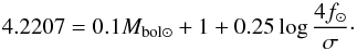 (10)Equation (9) can also be written as
  (11)where Sλ is defined by
  (12)Wesselink (1969), Parsons (1970), Barnes & Evans (1976), and Barnes et al. (1976, 1978) demonstrated using known angular diameters of stars, a correlation between Sλ, and color index C (mλ2 − mλ1) given by
  (13)where an are the polynomial coefficients of the calibration between Sλ and color index Cn.
For all our 150 models, we have thus obtained the surface brightness from Eq. (12) and the V − K color index from Eq. (5). Finally the calibration of these two quantities give the Eq. (13).
3.3. The M3 model as an example
We show in Fig. 5 how the V − K and Sv quantities associated with the M3 model (and C3 interferometric configuration) vary as a function of the rotation, the inclination, and also the projected rotational velocity Vrotsini. We can make several remarks:
-
1.
The higher the rotational velocity, the greater the bias comparedto the static model: can be as large as 0.1 mag inV − K color and/or surface brightness.
-
2.
The inclination angle essentially has an impact on the V − K color: i< 50° (resp. i> 50°) makes the star redder (resp. bluer). More particularly and very interestingly, regardless of its rotational velocity, as soon as a star is seen edge-on or pole-on, the interferometric bias in V − K and in surface brightness compensate in such a way that the star stands almost on the static SBCR.
-
3.
A model with a given projected rotational velocity Vrotsini can cover a large domain in V − K and in surface brightness, which introduces a significant bias compared to the static model. The lowest bias is found for stars with Vrotsini< 100 km s-1; in this case, the models stand reasonably close to the static relation.
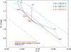 |
Fig. 5 Surface brightness versus the V − K color for the M3 model (Table 1), considering the C3 interferometric configuration (Table 2). The rotational velocity of the star is indicated in percentage of the critical rotational velocity (Vc), together with the inclination angle (in degrees). The corresponding projected rotational velocity Vrotsini are also indicated by dotted lines. The orange solid line is the SBCR found for the static models (see next section). The violet dotted line is the empirical SBCR from Challouf et al. (2014b), together with its dispersion (red dot-dashed line). |
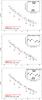 |
Fig. 6 Sv as function of V − K, for the 6 models of Table 1 rotating at 95% of their critical velocity and for different inclination angles: 0°, 25°, 50°, 75°, and 90° (blue points). The same but for edge-on models with different rotational velocity: 0.0Vc, 0.25Vc, 0.50Vc, 0.75Vc, and 0.95Vc (green points). Top: W2S2 (C1). Middle: W1W2E2 (C2). Below: W2S2-W1W2E2 (C3). The SBCR from Challouf et al. (2014b) is shown for comparison. |
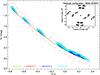 |
Fig. 7 Surface brightness versus the V − K color considering the C3 interferometric configuration for 150 models. The colors indicate the different velocity intervals. The black solid line is the SBCR found for the static models. The red dotted line is the empirical SBCR from Challouf et al. (2014b), together with its dispersion (red dot-dashed line). The (+) symbol presents the static models. |
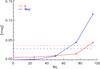 |
Fig. 8 Relation between the rotational velocity (as a percentage of the critical rotational velocity) and (1) the shift in zero point (Δa0) of the SBCR (compared to the static relation) and (2) its dispersion (σ). The horizontal red (resp. blue) dotted lines correspond to the average σ (resp. Δa0) for the 150 models (see Table 3). All the quantities are derived using the C3 interferometric configuration. |
4. Impact of the interferometric configuration on the SBCR
In this section, we consider the 150 computed models and derive their V − K and SV following the methodology described in Sect. 3. This is done for the three CHARA configurations C1, C2, and C3. The result is shown in Fig. 6. In this figure we do not show the 150 models for clarity, but only the 50 models corresponding to extreme cases in term of rotational velocity and inclination. In Table 3, we present the coefficients of the SBCR (polynomial fit of degree 3) for the three configurations, along with their dispersion (σ). The relation obtained for the six static models (rotational velocity of zero) is shown for comparison. We also use the difference of the zero points of the three relations for C1, C2, and C3, respectively, compared to the static SBCR, as an indicator of their average shift along the Y-axis: Δa0 = a0 [for Ci] −a0[static] in magnitude. It actually corresponds to the shift obtain at V − K = 0.
We can make the following remarks:
-
1.
We find that considering a baseline configuration along thepolar axis (resp. equatorial axis) produces a statistical bias of−0.05 (resp. 0.00) magnitude (along Y-axis) compared to the static SBCR. These values are extreme cases in the sense that our 150 models have their equatorial axis aligned with the east-west orientation on the sky. If the baseline configuration covers the (u, v) plan properly, then the bias has −0.03 mag.
-
2.
Regardless of the baseline configuration, the expected dispersion in the SBCR due to the rotation (rotational velocity and inclination) ranges from 0.04 (C3 configuration) to 0.06 (C1 configuration) magnitude. Interestingly, no matter what the interferometric configuration is, the large majority of the 150 models lie within the dispersion (0.16 mag) of the empirical SBCR found by Challouf et al. (2014b).
-
3.
When the star is seen edge-on and whatever the rotational velocity, the SBCR is almost on the static relation when we take the best covering (u, v) plane (Fig. 6 below).
-
4.
The static SBCR relation is consistent with the empirical one from Challouf et al. (2014b), which is within a +/− σ = 0.16 mag. empirical uncertainty.
We now consider our six samples of models with rotational velocities of 0, 25, 50, 75, and 95% of the critical rotational velocity, respectively (thus 30 models per sample). In Fig. 7, we show the 150 models with their respective rotational velocities, as in Fig. 5 but interpolated for each interval of velocity and illustrated by a color. All models within a given interval of velocity (i.e., one sample of 30 models) is fitted with a polynomial function of degree 3, and the results are given in Table 3. The corresponding Δa0 values and dispersion of these SBCR relations are indicated in the table and illustrated in Fig. 8.
Calibration of SBCR for different rates of rotational velocities with the following function Sv = a0 + a1(V − K) + a2(V − K)2 + a3(V − K)3.
We find a clear relation between the rotational velocity and (1) the shift in zero point (Δa0) of the SBCR (compared to the static relation) and (2) its dispersion (σ). When considering stars rotating at less than 50% of their critical velocity, Δa0 and σ have about a 0.01 mag, while these quantities can reach 0.08 and 0.04 mag, respectively, when the rotation is more than 75% of the critical velocity. The dashed lines are the same quantities but considering the 150 models for C3 (see previous section).
5. Conclusion
In this paper we aimed at theoretically quantifying the impact of fast rotation on the SBCR of early-type stars. After verifying that the static theoretical and empirical (Challouf et al. 2014b) SBCR relations are roughly consistent, we concluded that the rotational velocity and the inclination (compare to the line of sight) of the stars result in a dispersion of the SBCR of about 0.04 mag and a bias of about the same value, 0.03 mag. These values are slightly but not significantly changed (about 0.03 and 0.01 mag in Δa0 and σ, respectively) when considering different CHARA configurations. Finally, all our models (regardless of the interferometric configuration) are consistent with the 0.16 mag dispersion of the empirical SBCR found by Challouf et al. (2014b). This does not mean that the 0.16 mag of dispersion is entirely due to rotation, but most certainly that rotation is one of the various physical effects (along with mass loss and environment) that is contributing to the dispersion of the SBCR. We also notice that the bias (or zero-point shifts) due to the interferometric configuration (from 0 to 0.05 mag) are lower than the observed dispersion, which explains why rotating stars have been used up to now to calibrate the SBCR: the bias due to rotation was indeed within the uncertainties and not seen in the data analysis.
The aim of this work is to improve the SBCR of early-type stars. In the framework of the Araucaria project, we need a SBCR for early-type stars as precise as 1% or 0.02 mag in order to derive the distance in the local group of bright early-type eclipsing binaries, which are not affected by the rotation in principle. To reach such objective, our suggestion is (1) to use a decent (u, v) coverage; (2) observe a large sample of rotating early-type stars again by interferometry (most preferably in the visible because these stars are generally small angularly) with rotational velocities lower than 50 km s-1; (3) secure new and homogeneous optical and infrared photometry to calibrate the SBCR relation. Alternatively, if one cannot determine the rotational velocity of the stars, our calculations show that considering stars with projected rotational velocity Vrotsini lower than 100 km s-1result in a zero-point shift of Δa0 = 0.02 mag and a dispersion of σ = 0.03 mag, respectively.
CHARA: Center for High Angular Resolution Astronomy.
Acknowledgments
This research made use of the SIMBAD and VIZIER databases at the CDS, Strasbourg France (http://cdsweb.u- strasbg.fr/), and of the electronic bibliography maintained by the NASA/ADS system. The research leading to these results has received funding from the European Community’s Seventh Framework Program under Grant Agreement 312430 and financial support from the Ministry of Higher Education and Scientific Research (MHESR) – Tunisia. W.G. and G.P. gratefully acknowledge support for this work from the BASAL Centro de Astrofisica y Tecnologias Afines (CATA) PFB-06/2007. W.G. also acknowledges support from the Chilean Ministry of Economy, Development and Tourism’s Millenium Science Initiative through grant IC 120009 awarded to the Millenium Institute of Astrophysics (MAS). Support from the Polish National Science Center grant MAESTRO 2012/06/A/ST9/00269 is also acknowledged.
References
- Allen de Prieto, C., & Lambert, D. L. 1999, A&A, 352, 555 [NASA ADS] [Google Scholar]
- Barnes, T. G., & Evans, D. S. 1976, MNRAS, 174, 489 [NASA ADS] [CrossRef] [Google Scholar]
- Barnes, T. G., Evans, D. S., & Parsons, S. B. 1976, MNRAS, 174, 503 [NASA ADS] [CrossRef] [Google Scholar]
- Barnes, T. G., Evans, D. S., & Moffett, T. J. 1978, MNRAS, 183, 285 [NASA ADS] [CrossRef] [Google Scholar]
- Bohm-Vitense, E. 1985, ApJ, 296, 169 [NASA ADS] [CrossRef] [Google Scholar]
- Bonanos, A. Z., Stanek, K. Z., Kudritzki, R. P., et al. 2006, ApJ, 652, 313 [NASA ADS] [CrossRef] [Google Scholar]
- Challouf, M., Nardetto, N., Mourard, D., Aroui, H., & Chesneau, O. 2012, in SF2A-2012: Proc. Annual meeting of the French Society of Astronomy and Astrophysics, eds. S. Boissier, P. de Laverny, N. Nardetto, et al., 299 [Google Scholar]
- Challouf, M., Nardetto, N., Mourard, D., Aroui, H., & Delaa, O. 2014a, in SF2A-2014: Proc. Annual meeting of the French Society of Astronomy and Astrophysics, eds. J. Ballet, F. Martins, F. Bournaud, R. Monier, & C. Reylé, 471 [Google Scholar]
- Challouf, M., Nardetto, N., Mourard, D., et al. 2014b, A&A, 570, A104 [NASA ADS] [CrossRef] [EDP Sciences] [Google Scholar]
- Challouf, M., Nardetto, N., Domiciano de Souza, A., et al. 2015, in IAU Symp., 307, 288 [Google Scholar]
- Che, X., Monnier, J. D., Zhao, M., et al. 2011, ApJ, 732, 68 [NASA ADS] [CrossRef] [Google Scholar]
- Claret, A. 2012, A&A, 538, A3 [NASA ADS] [CrossRef] [EDP Sciences] [Google Scholar]
- Claret, A., & Bloemen, S. 2011, A&A, 529, A75 [NASA ADS] [CrossRef] [EDP Sciences] [Google Scholar]
- Domiciano de Souza, A., Vakili, F., Jankov, S., Janot-Pacheco, E., & Abe, L. 2002, A&A, 393, 345 [NASA ADS] [CrossRef] [EDP Sciences] [Google Scholar]
- Domiciano de Souza, A., Hadjara, M., Vakili, F., et al. 2012a, A&A, 545, A130 [NASA ADS] [CrossRef] [EDP Sciences] [Google Scholar]
- Domiciano de Souza, A., Zorec, J., & Vakili, F. 2012b, in SF2A-2012: Proc. Annual meeting of the French Society of Astronomy and Astrophysics, eds. S. Boissier, P. de Laverny, N. Nardetto, et al., 321 [Google Scholar]
- Domiciano de Souza, A., Kervella, P., Moser Faes, D., et al. 2014, A&A, 569, A10 [NASA ADS] [CrossRef] [EDP Sciences] [Google Scholar]
- Espinosa Lara, F., & Rieutord, M. 2011, A&A, 533, A43 [NASA ADS] [CrossRef] [EDP Sciences] [Google Scholar]
- Evans, N. R. 1991, ApJ, 372, 597 [NASA ADS] [CrossRef] [Google Scholar]
- Evans, N. R. 1992, ApJ, 389, 657 [NASA ADS] [CrossRef] [Google Scholar]
- Graczyk, D., Soszyński, I., Poleski, R., et al. 2011, Acta Astron., 61, 103 [NASA ADS] [Google Scholar]
- Hanbury Brown, R., Davis, J., Lake, R. J. W., & Thompson, R. J. 1974, MNRAS, 167, 475 [NASA ADS] [CrossRef] [Google Scholar]
- Hubeny, I., & Lanz, T. 2011, Astrophysics Source Code Library [record ascl:1109.022] [Google Scholar]
- Kurucz, R. L. 1979, ApJS, 40, 1 [NASA ADS] [CrossRef] [Google Scholar]
- Macri, L. M., Stanek, K. Z., Sasselov, D. D., Krockenberger, M., & Kaluzny, J. 2001, AJ, 121, 870 [NASA ADS] [CrossRef] [Google Scholar]
- Mochejska, B. J., Kaluzny, J., Stanek, K. Z., & Sasselov, D. D. 2001, AJ, 122, 1383 [NASA ADS] [CrossRef] [Google Scholar]
- Monnier, J. D., Zhao, M., Pedretti, E., et al. 2007, Science, 317, 342 [NASA ADS] [CrossRef] [PubMed] [Google Scholar]
- Mourard, D., Clausse, J. M., Marcotto, A., et al. 2009, A&A, 508, 1073 [NASA ADS] [CrossRef] [EDP Sciences] [Google Scholar]
- Mourard, D., Bério, P., Perraut, K., et al. 2011, A&A, 531, A110 [NASA ADS] [CrossRef] [EDP Sciences] [Google Scholar]
- Mourard, D., Challouf, M., Ligi, R., et al. 2012, in SPIE Conf. Ser., 8445 [Google Scholar]
- Paczynski, B., & Stanek, K. Z. 1998, ApJ, 494, L219 [NASA ADS] [CrossRef] [Google Scholar]
- Parsons, S. B. 1970, ApJ, 159, 951 [NASA ADS] [CrossRef] [Google Scholar]
- Pawlak, M., Graczyk, D., Soszyński, I., et al. 2013, Acta Astron., 63, 323 [NASA ADS] [Google Scholar]
- Peterson, D. M., Hummel, C. A., Pauls, T. A., et al. 2006, ApJ, 636, 1087 [NASA ADS] [CrossRef] [Google Scholar]
- Pietrzyński, G., Thompson, I. B., Graczyk, D., et al. 2009, ApJ, 697, 862 [NASA ADS] [CrossRef] [Google Scholar]
- Pietrzyński, G., Graczyk, D., Gieren, W., et al. 2013, Nature, 495, 76 [NASA ADS] [CrossRef] [PubMed] [Google Scholar]
- Stanek, K. Z., & Garnavich, P. M. 1998, ApJ, 503, L131 [NASA ADS] [CrossRef] [Google Scholar]
- ten Brummelaar, T. A., McAlister, H. A., Ridgway, S. T., et al. 2005, ApJ, 628, 453 [NASA ADS] [CrossRef] [Google Scholar]
- Udalski, A. 2000, ApJ, 531, L25 [NASA ADS] [CrossRef] [PubMed] [Google Scholar]
- van Belle, G. T. 2012, A&ARv, 20, 51 [NASA ADS] [CrossRef] [Google Scholar]
- van Belle, G. T., Ciardi, D. R., Thompson, R. R., Akeson, R. L., & Lada, E. A. 2001, ApJ, 559, 1155 [NASA ADS] [CrossRef] [MathSciNet] [Google Scholar]
- van Cittert, P. H. 1934, Physica, 1, 201 [NASA ADS] [CrossRef] [Google Scholar]
- Vilardell, F., Ribas, I., & Jordi, C. 2006, A&A, 459, 321 [NASA ADS] [CrossRef] [EDP Sciences] [Google Scholar]
- Von Zeipel, H. 1924, MNRAS, 84, 665 [NASA ADS] [CrossRef] [Google Scholar]
- Wesselink, A. J. 1969, MNRAS, 144, 297 [NASA ADS] [CrossRef] [Google Scholar]
- Worthey, G., & Lee, H.-c. 2011, ApJS, 193, 1 [NASA ADS] [CrossRef] [EDP Sciences] [Google Scholar]
- Wyrzykowski, L., Udalski, A., Kubiak, M., et al. 2003, Acta Astron., 53, 1 [NASA ADS] [CrossRef] [Google Scholar]
- Wyrzykowski, L., Udalski, A., Kubiak, M., et al. 2004, Acta Astron., 54, 1 [NASA ADS] [CrossRef] [Google Scholar]
- Zernike, F. 1938, Physica, 5, 785 [NASA ADS] [CrossRef] [Google Scholar]
- Zhao, M., Monnier, J. D., Pedretti, E., et al. 2009, ApJ, 701, 209 [NASA ADS] [CrossRef] [Google Scholar]
All Tables
Calibration of SBCR for different rates of rotational velocities with the following function Sv = a0 + a1(V − K) + a2(V − K)2 + a3(V − K)3.
All Figures
|
Fig. 1 Left: modeled intensity distributions; Right: the Fourier transform of the intensity map of M1 at 720 nm for 95% of Vc and i = 90°. |
| In the text | |
|
Fig. 2 Configuration of the CHARA array (ten Brummelaar et al. 2005) located at the Mount Wilson Observatory, north of Los Angeles (California, USA). The CHARA array consists of 6 telescopes of 1 meter in diameter, configured in a Y-shape, which offers 15 different baselines from 34 m to 331 m. |
| In the text | |
|
Fig. 3 Top: intensity maps are given in units of the equatorial radius (Req) with the project baselines in the sky. Bottom: squared visibility versus spatial frequency. The figures calculated for inclination (from left to right): 0°, 25°, 50°, 75°, and 90°. The rotational velocity for all inclinations is of 0.95Vc. The visibilities points presented with same color bases of Fig. 2, and the red lines are the best fitted uniform disk. The mean angular diameter θUD ranges from 0.635 ± 0.006 mas to 0.736 ± 0.001 mas. |
| In the text | |
|
Fig. 4 Top: intensity maps given in units of the equatorial radius (Req) with the project baselines in the sky. Bottom: squared visibility versus spatial frequency. The figures calculated for rotational velocities (from left to right): 0.0Vc, 0.25Vc, 0.50Vc, 0.75Vc, and 0.95Vc. The inclination for all rotational velocities is 90°. The visibilities points presented with same color bases as in Fig. 2, and the red lines are the best-fitted uniform disk. The mean angular diameter θUD ranges from 0.635 ± 0.006 mas to 0.782 ± 0.001 mas. |
| In the text | |
|
Fig. 5 Surface brightness versus the V − K color for the M3 model (Table 1), considering the C3 interferometric configuration (Table 2). The rotational velocity of the star is indicated in percentage of the critical rotational velocity (Vc), together with the inclination angle (in degrees). The corresponding projected rotational velocity Vrotsini are also indicated by dotted lines. The orange solid line is the SBCR found for the static models (see next section). The violet dotted line is the empirical SBCR from Challouf et al. (2014b), together with its dispersion (red dot-dashed line). |
| In the text | |
|
Fig. 6 Sv as function of V − K, for the 6 models of Table 1 rotating at 95% of their critical velocity and for different inclination angles: 0°, 25°, 50°, 75°, and 90° (blue points). The same but for edge-on models with different rotational velocity: 0.0Vc, 0.25Vc, 0.50Vc, 0.75Vc, and 0.95Vc (green points). Top: W2S2 (C1). Middle: W1W2E2 (C2). Below: W2S2-W1W2E2 (C3). The SBCR from Challouf et al. (2014b) is shown for comparison. |
| In the text | |
|
Fig. 7 Surface brightness versus the V − K color considering the C3 interferometric configuration for 150 models. The colors indicate the different velocity intervals. The black solid line is the SBCR found for the static models. The red dotted line is the empirical SBCR from Challouf et al. (2014b), together with its dispersion (red dot-dashed line). The (+) symbol presents the static models. |
| In the text | |
|
Fig. 8 Relation between the rotational velocity (as a percentage of the critical rotational velocity) and (1) the shift in zero point (Δa0) of the SBCR (compared to the static relation) and (2) its dispersion (σ). The horizontal red (resp. blue) dotted lines correspond to the average σ (resp. Δa0) for the 150 models (see Table 3). All the quantities are derived using the C3 interferometric configuration. |
| In the text | |
Current usage metrics show cumulative count of Article Views (full-text article views including HTML views, PDF and ePub downloads, according to the available data) and Abstracts Views on Vision4Press platform.
Data correspond to usage on the plateform after 2015. The current usage metrics is available 48-96 hours after online publication and is updated daily on week days.
Initial download of the metrics may take a while.