© ESO, 2015

1. Introduction

Magnetohydrodynamic transverse waves seem to be a relevant constituent of the dynamics of magnetic and plasma structures in the solar atmosphere. Their presence has been invoked to explain imaging and spectroscopic signatures of periodic plasma motions detected in different types of structures with different physical conditions, such as coronal loops (Aschwanden et al. 1999; Nakariakov et al. 1999), chromospheric spicules and mottles (De Pontieu et al. 2007), soft X-ray coronal jets (Cirtain et al. 2007), prominence fine structures (Okamoto et al. 2007; Lin et al. 2009), or extended regions of the solar corona (Tomczyk et al. 2007). In recent years, their relevance has increased because of their potential as a tool for seismic diagnosis (Arregui et al. 2007; Goossens et al. 2008; Arregui & Asensio Ramos 2011; Nakariakov & Ofman 2001; De Moortel & Nakariakov 2012) and because of their possible role in the wave heating processes (Parnell & De Moortel 2012; Arregui 2015).

López Ariste et al. (2013) demonstrated that there are solutions to the equation of magneto-hydrodynamic waves carrying wavefront dislocations. In that work, the equation studied was Eq. (4.14) from Priest (1982), which reads as $\frac{{\mathit{\partial }}^{\mathrm{2}}{{v}}_{\mathrm{1}}}{\mathit{\partial }{\mathit{t}}^{\mathrm{2}}}\mathrm{=}{\mathit{c}}_{\mathit{S}}^{\mathrm{2}}{\nabla }\mathrm{\left(}{\nabla }{{v}}_{\mathrm{1}}\mathrm{\right)}\mathrm{+}\left[{\nabla }\mathrm{\times }\mathrm{(}{\nabla }\mathrm{\times }\mathrm{(}{{v}}_{\mathrm{1}}\mathrm{\times }{{B}}_{\mathrm{0}}\mathrm{\left)}\mathrm{\right)}\right]\mathrm{\times }\frac{{{B}}_{\mathrm{0}}}{\mathit{\mu }{\mathit{\rho }}_{\mathrm{0}}}\mathit{,}$(1)where v₁ is the velocity of the plasma, B₀ the magnetic field (assumed constant), c_S the speed of sound in the medium, and ρ₀ the density. This equation describes linear magnetohydrodynamical waves in a homogeneous, isothermal medium. As solutions, this equation has waves propagating along the magnetic field that carry wavefront dislocations (Nye & Berry 1974), that is, singularities in the phase of the wave. Examples of such waves can be seen in Fig. 1. The four images show different kinds of dislocations made by varying the parameters β and δ of a generic solution to the longitudinal (that is, along the magnetic field) component of the velocity perturbation v_z in Eq. (1) given by López Ariste et al. (2013): ${\mathit{v}}_{\mathit{z}}\mathrm{=}\mathit{A}\mathrm{(}\mathit{k}{\mathit{r}}^{\mathit{m}}{\mathrm{e}}^{\mathrm{i}\mathit{m\theta }}\mathrm{+}\mathit{\beta }{\mathrm{e}}^{\mathrm{i}\mathit{\delta }}\mathit{k}\mathrm{(}\mathit{z}\mathrm{-}\mathit{ct}{\mathrm{\left)}}^{\mathrm{\right)}}{\mathrm{e}}^{\mathrm{i}\mathit{k}\mathrm{(}\mathit{z}\mathrm{-}\mathit{ct}\mathrm{)}}\mathit{.}$(2)Starting from the left, the illustrated dislocations are a pure vortex (β = 0), two pure edge dislocations ($\mathit{\beta }\ne \mathrm{0}\mathit{,\delta }\mathrm{=}\frac{\mathit{\pi }}{\mathrm{2}}$), and a mixture of vortex and edge that can be described as a gliding dislocation (β ≠ 0,δ = 0). The axes of the plot are time and distance, though any other sensitive choice can be made that captures the topology of the wavefront under scrutiny.

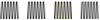Fig. 1 Four examples of dislocations in the propagation of a wave with the time in abscissas and a distance in ordinates. From left to right, a vortex, two edges, and a gliding edge, all with charge 1. Around the second edge dislocation, a closed curve has been drawn with dots and squares. The integral of the phase along this curve, the monodromy, is non-zero.

When looking at this kind of picture, it is important to agree that the quasi-periodic variation seen in those time-distance plots is a sound representation of the phase of the wave times an amplitude that does not have to be constant over the plot. (Actually it will be zero at the singularity and only at that point, but can take any other value elsewhere.) A wave period can be measured with more or less precision and significance by measuring the distance between two crests (white color) or two valleys (black color) in such a plot. If we were staring at a plane wave, the pattern of black and white crests and valleys of the wave would be roughly parallel over the plot.

We see that this is not the case so we circled a particular region in one of the figures in which one crest ends suddenly where two valleys merge into just one. It is evident that the ending point of that crest cannot have a well-defined phase, so it is singular. The amplitude of the wave at this point should be zero. This is the dislocation. Sometimes it is just a point (pure edge dislocation), but often it is a line of singularities (as in the vortex case on the leftmost figure or the gliding dislocation of the rightmost one).

At this point it is important to distinguish a dislocation from mere wave nodes. A node is just a zero of a wave with real amplitude. It is often illustrated in one-dimensional plots of waves, or else in two interfering waves as in standing waves, where we see the amplitude go to zero. But this definition makes no mention of the phase of the wave, which despite the zero amplitude, may still be perfectly well defined. In a dislocation the phase of the wave is singular. Thus, dislocations can be seen as nodes, but not all nodes are dislocations. An illustration is offered in our context of MHD waves by the solution of a wave propagating along the z direction and by the transverse plane (r,θ) having the form J₁(r)e^iθ.

Each zero of the Bessel function J₁ is a node of the wave: the amplitude will be zero at those places at all times. But the node at r = 0 is a dislocation since the phase θ is undefined or singular at that point. In contrast the first zero at r = 3.83 is a node for which the phase is perfectly well defined, so it is not a dislocation. Distinguishing a dislocation from a node with a wave given as a real function of just one variable is not possible. If the wave is written as a complex function ρe^iχ = a + ib, the dislocation is found as that place where a = b = 0, which immediately leaves the phase $\mathit{\chi }\mathrm{=}\arctan \frac{\mathit{b}}{\mathit{a}}$ singular and the amplitude $\mathit{\rho }\mathrm{=}\sqrt{{\mathit{a}}^{\mathrm{2}}\mathrm{+}{\mathit{b}}^{\mathrm{2}}}$ zero. If the wave is seen as a function of two variables (time and one spatial dimension) as in our examples of Figs. 1 or 2, the qualitative description made above also successfully identifies a dislocation and separates it from other nodes.

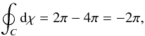
This qualitative picture of a dislocation in a time-distance plot of the wavefront or the simple rule of finding the places where both the imaginary and real parts of the waves are simultaneously zero must be complemented by a more quantitative and mathematically rigorous definition of the singularity. This is done by drawing a closed curve, called a monodromy, along which we integrate an appropriate parameter. In our case the monodromy is computed over the phase: if we describe the wave as a map of ρe^iχ, with ρ and χ real numbers that define the amplitude and phase, respectively, at each and every point, the monodromy of interest is

${\mathrm{􏽉}}_{\mathit{C}}\mathrm{d}\mathit{\chi }$where C represents that closed curve that can be in our example the circle around the singularity. The monodromy is strictly zero when there is no singularity in the area enclosed by C, and it is 2πm if there is a dislocation, with m the topological charge of the singularity. This charge m is named to coincide with the m in Eq. (2). And this is on purpose, since we verify that the m in that solution defines the charge of the generated dislocation.

López Ariste et al. (2013) pointed to observations of magnetoacoustic waves in the sunspot umbra by Centeno et al. (2006) where dislocations like those illustrated could be easily identified visually but also by computing the monodromy. Dislocations are not extraordinary solutions of the wave equation but actually quite common occurrences, as those observations demonstrated. In the scenario described by Eq. (1), there is a clear axial symmetry given by the constant magnetic field. If, for the time being, we restrict ourselves to waves propagating along this z direction, it is well known (Wentzel 1979; Spruit 1982; Edwin & Roberts 1983; Roberts 1981) that solutions to this equation are given in terms of families of Bessel functions times an azimuthal dependence e^imθ. This angle θ corresponding to the cylindrical azimuth coordinate is obviously singular at the origin of the coordinate system r = 0. Those classic solutions to the Eq. (1) therefore carry a dislocation at r = 0 for all the cases with m ≠ 0.

We find here a third occurrence of m, this time for referring to the azimuthal wave number of the solutions to the wave equation. It is sufficient to try the monodromy integral over the gradient of the phase to realize that m is exactly the charge of the dislocation introduced above. And thus, following the usual naming convention, a wave with charge m = 0 will be called a sausage mode, while a wave with charge m = 1 will be called a kink mode. Higher values of the charge m are referred to as flute modes. Finally, it is interesting to notice and stress at this point that any attempt to describe such singularities with a finite combination of colinear plane waves or Fourier components will fail. Dislocations require either the full infinite series of the Fourier decomposition or a choice of a family of solutions that already carries a dislocation in each or most of its components. The Bessel functions times the azimuthal dependence e^imθ are one of these families, and they offer an example that we should expect to find in the description of magnetohydrodynamic waves in the solar atmosphere. It is therefore expected that dislocations are observed in waves in the solar atmosphere, though the common description of waves in terms of plane waves have resulted in overlooking them because plane waves cannot describe dislocations.

In the present paper we should turn to another observation of magnetohydrodynamic waves, this time in the solar corona. The observations can be seen in Fig. 2, and they will be described in terms of dislocations in the next section. Section 3 is a first attempt to describe the observed dislocations in terms of generic wave solutions that require the presence of several interfering waves with different frequencies and propagation velocities. The detailed inspection of mathematical solutions in Sect. 4 will show that although most of the waves propagating in coronal tubes carry dislocations, they are not visible in observations like the one in Fig. 2 unless the observed Doppler velocity is a projection of both the transverse and the longitudinal velocity. This last one therefore must be non-zero, which implies the necessary presence of at least one magnetoacoustic mode in the observed waves.

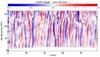Fig. 2 Observation of coronal waves in the Doppler velocity of a coronal emission line by COMP from Threlfall et al. (2013). The diagram has time in abscissas and the coordinate z, along the loop and parallel to the magnetic field, in ordinates. Among the many visible dislocations, two have been labeled. The closed curve (that could represent the monodromy) encloses an edge dislocation, while the straight segment follows a possible gliding dislocation.

2. Dislocations observed in waves propagating along coronal tubes

Figure 2 shows a plot of measured Doppler velocities as a function of time for a particular trajectory in the corona, measured in a coronal emission line by the Coronal Multi-channel Polarimeter (CoMP, Tomczyk et al. 2008). The observations were presented by Threlfall et al. (2013; see also Tomczyk et al. 2007; Tomczyk & McIntosh 2009). The parameters of the observation, off the solar disk, imply that we are observing here the velocity of the emitting plasma roughly transverse to the direction of the coronal magnetic field. The periodicity of the signal is evident. An average frequency ω can be estimated, and we should use it throughout this paper to describe a carrier wave whose amplitude and phase may be locally modified.

Another clear feature of the observed waves is the tilt of some of the crests and valleys, which indicate a propagating wave along the coronal feature and along the magnetic field (Threlfall et al. 2013). Several dislocations are also more visible after comparing them with the previous examples. We marked one of them around minute 55, as in Fig. 1, with a closed curve made of four segments. A monodromy of interest would be the integration of the phase of the wave along this closed curve. If this integral is not zero, the enclosed pattern will contain a dislocation. However, Fig. 2 shows the actual Doppler shift or velocity of the plasma, not its phase. We therefore cannot integrate the measured values directly over the curve.

In the Appendix we show how the computation of the integral directly from the data can be made, but here we take a more heuristic approach: one can always deform the curve so that it is made of four segments along which we can safely identify the phase of the wave or its changes from the observations and integrate these inferred values. The first such segment follows the blue valley to the left of the dislocation from roughly position 130 to position 50 in the ordinates. We draw this segment so as to follow Phase 0. (We assume that valleys are at Phase 0 and crests at Phase π.) Given the interpretation of these blue and red stripes as the valleys and crests of a wave, we should also agree that roughly at the center of the referred valley there is a continuous line at Phase 0 over which we draw the segment.

A similar segment is drawn over the next blue valley to the right, also along the 0-phase value. The integral ^∫dχ along either one of these two segments is 0 since there is no change in phase. We then join the two segments with a straight horizontal line at ordinates position 50 from left to right. This straight horizontal segment goes from a point at Phase 0 to the next red crest at Phase π and then ends in the next valley at Phase 2π ≡ 0. The integral ^∫dχ = 2π along this segment. Similarly, at ordinate point 130 we draw a horizontal and a straight line from right to left joining the two vertical blue segments. This time the horizontal line starts at Phase 0 and goes over two red crests and one blue valley before ending up in the final blue valley where we drew the segment. The integral is ^∫dχ = −2 × 2π, where the minus sign comes from going from right to left, rather than in the other direction. The full integral along this closed curve is therefore

${\mathrm{􏽉}}_{\mathit{C}}\mathrm{d}\mathit{\chi }\mathrm{=}\mathrm{2}\mathit{\pi }\mathrm{-}\mathrm{4}\mathit{\pi }\mathrm{=}\mathrm{-}\mathrm{2}\mathit{\pi ,}$which is different than zero. As a result, it has a charge m = −1, given the chosen orientation of the curve. A direct computation of the integral confirms the result, as seen in the Appendix. From the theory of functions of complex variable, a closed integral over a function of complex variables is non-zero when it encloses a number of poles or singularities larger than the number of zeros. We conclude that somewhere inside this closed curve, there is a singularity that results in a nonzero, nontrivial monodromy.

This computation of the monodromy can be repeated for many other similar points in the figure, in particular for the line of dislocations that we identify as a possible gliding dislocation after comparison with Fig. 1. On the other hand, the main dislocation, whose monodromy we computed, appears to be an edge type. No pure vortex is seen. To explain these dislocations, it is important to stress that the axes of the plot are time t and distance z along a coronal loop as projected onto the plane of the sky. The edge dislocations seen in the figure are therefore localized at particular values of t and z, but there is no constraint on their position in the transverse plane, i.e., on the values of the transverse coordinates x,y (or r,θ in the more appropriate cyclindric reference system).

Other assumed constraints beyond z being along the loop (Threlfall et al. 2013) are that the magnetic field follows the coronal loop and that the wave propagates along this magnetic field. Since coronal loops appear as structures in coronal emission lines whose intensity variations are related to density enhancements, we further assume that the wave is propagating in a high-density cylinder. The phase speed of the propagating wave has been measured to be in the range 700−1000 km s^-1. Such speeds are much higher than the sound speed of the corona and are comparable to the Alfvén and kink speeds characteristic of the propagation of Alfvén waves and fast magnetoacoustic body waves in coronal loops, respectively.

3. Interpretation of the observed dislocations in coronal waves

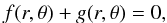
A dislocation is a phase singularity. At the exact point of the phase singularity, the amplitude of the complex wave has to be zero. This statement allows us to search for dislocations as zeros of the complex amplitude of the wave. We want to describe a wave ψ propagating at a characteristic frequency ω and wavenumber k along the z axis, parallel to the magnetic field and the coronal loop. One common form for the solution of such a wave is written as

$\mathit{\psi }\mathrm{=}\mathit{f}\mathrm{\left(}\mathit{r,\theta ,z,t}\mathrm{\right)}{\mathrm{e}}^{\mathrm{i}\mathrm{(}\mathit{kz}\mathrm{-}\mathit{\omega t}\mathrm{)}}\mathit{.}$We notice that f may depend on the three cylindric coordinates and on time, in the most general case. Since the term e^i(kz−ωt) can be neither zero nor singular, it is obvious that all the information on the dislocations of this wave is contained in the f function that should be complex in general. We are therefore looking for those times and places (r,θ,z,t) where the complex amplitude

$\mathrm{\parallel }\mathit{f}\mathrm{\left(}\mathit{r,\theta ,z,t}\mathrm{\right)}\mathrm{\parallel }\mathrm{=}\mathrm{0.}$A plane wave would have

$\mathit{f}\mathrm{\left(}\mathit{r,\theta ,z,t}\mathrm{\right)}\mathrm{=}\mathit{A,}$with A real. This amplitude cannot be zero, unless A = 0. Plane waves carry no dislocations therefore.

All the analytical solutions found and given for magnetohydrodynamic waves in coronal loops (Edwin & Roberts 1983; Priest 1982; Roberts 1981; Goossens et al. 2012, 2009) can be written as $\mathit{\psi }\mathrm{=}\mathit{f}\mathrm{\left(}\mathit{r,\theta }\mathrm{\right)}{\mathrm{e}}^{\mathrm{i}\mathrm{(}\mathit{kz}\mathrm{-}\mathit{\omega t}\mathrm{)}}$(3)with no dependence of f on either z or time. This simplification can be justified in the case of homogeneous loops along the magnetic field and are constant in time, at least for periods that are longer than the period of the wave. This assumption also makes it possible to determine and fix ω and k. The actual form of the function f(r,θ) changes with the assumptions and physical phenomena considered, but it always retains these dependencies. If such a wave carries a dislocation, where the phase is singular, it will be found at those points (r,θ) where the amplitude of the wave satisfies the condition

$\mathrm{\parallel }\mathit{f}\mathrm{\left(}\mathit{r,\theta }\mathrm{\right)}\mathrm{\parallel }\mathrm{=}\mathrm{0.}$This equation will be valid for all values of z and t. The dislocation therefore will be localized in the transverse plane (r,θ) but not in the plot (z,t) of Fig. 2.

This is exactly the opposite situation to the one observed. The description of the wave as f(r,θ)e^i(kz−ωt) cannot produce a point dislocation in the plane (z,t) and cannot therefore describe Fig. 2, independently of the actual form of f(r,θ). In view of this and since the observed dislocations are certainly localized in (z,t), we may doubt the description of the wave given in Eq. (3). Waves propagating along the field have to have this functional form as long as the assumptions made above hold, so we could as an alternative consider that the observed wave is propagating across the field. This possibility was, however, quickly discarded after inspection of the possible analytical solutions to such a wave. We are not going to give the details here.

Another possibility we have inspected is that what we are observing is the interference of more than one wave. This possibility has been put forward by Threlfall et al. (2013) and Tomczyk & McIntosh (2009) from actual inspection and Fourier filtering of the observations. Although it is unclear whether the methods used by those authors are still valid in the presence of phase singularities, let us follow them and suggest the possibility of two waves propagating with different frequencies ω₁ and ω₂. We further assume that the frequency difference Δω = ω₂−ω₁ is small, since Threlfall et al. (2013) filtered the observations in the Fourier space. This wave can be written as 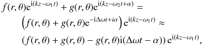$\begin{array}{ccc}& & \mathit{f}\mathrm{\left(}\mathit{r,\theta }\mathrm{\right)}{\mathrm{e}}^{\mathrm{i}\mathrm{(}\mathit{kz}\mathrm{-}{\mathit{\omega }}_{\mathrm{1}}\mathit{t}\mathrm{)}}\mathrm{+}\mathit{g}\mathrm{\left(}\mathit{r,\theta }\mathrm{\right)}{\mathrm{e}}^{\mathrm{i}\mathrm{(}\mathit{kz}\mathrm{-}{\mathit{\omega }}_{\mathrm{2}}\mathit{t}\mathrm{+}\mathit{\alpha }\mathrm{)}}\mathrm{=}\\ & & \mathrm{(}\mathit{f}\mathrm{\left(}\mathit{r,\theta }\mathrm{\right)}\mathrm{+}\mathit{g}\mathrm{\left(}\mathit{r,\theta }\mathrm{\right)}{\mathrm{e}}^{\mathrm{-}\mathrm{i\Delta }\mathit{\omega t}\mathrm{+}\mathit{i\alpha }}\mathrm{)}{\mathrm{e}}^{\mathrm{i}\mathrm{(}\mathit{kz}\mathrm{-}{\mathit{\omega }}_{\mathrm{1}}\mathit{t}\mathrm{)}}\mathrm{\approx }\\ & & \left(\mathit{f}\mathrm{\left(}\mathit{r,\theta }\mathrm{\right)}\mathrm{+}\mathit{g}\mathrm{\left(}\mathit{r,\theta }\mathrm{\right)}\mathrm{-}\mathit{g}\mathrm{\left(}\mathit{r,\theta }\mathrm{\right)}\mathrm{i}\mathrm{(}\mathrm{\Delta }\mathit{\omega t}\mathrm{-}\mathit{\alpha }\mathrm{)}\right){\mathrm{e}}^{\mathrm{i}\mathrm{(}\mathit{kz}\mathrm{-}{\mathit{\omega }}_{\mathrm{1}}\mathit{t}\mathrm{)}}\mathit{,}\end{array}$(4)which is a complex amplitude multiplying the propagation term e^{i(kz−ω₁t)}. Assuming for simplicity, but without loss of generality, that f and g are real amplitudes, we find that this wave can carry a dislocation when the two conditions 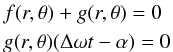$\begin{array}{ccc}& & \mathit{f}\mathrm{\left(}\mathit{r,\theta }\mathrm{\right)}\mathrm{+}\mathit{g}\mathrm{\left(}\mathit{r,\theta }\mathrm{\right)}\mathrm{=}\mathrm{0}\\ & & \mathit{g}\mathrm{\left(}\mathit{r,\theta }\mathrm{\right)}\mathrm{(}\mathrm{\Delta }\mathit{\omega t}\mathrm{-}\mathit{\alpha }\mathrm{)}\mathrm{=}\mathrm{0}\end{array}$(5)are simultaneously satisfied. The two equations are the real and imaginary parts of the complex amplitude of the wave. If we require that both are simultaneously zero, we find that the real amplitude of the wave is zero and that the phase is undefined, hence a dislocation. The second one of those equations, the one for the imaginary part, is immediately satisfied at t = −α/ Δω (modulo π), so this wave may carry a dislocation localized in time at the position (r,θ) where the real part of the complex amplitude is also zero. It is sufficient that two waves, even plane waves, with slightly different frequencies interfere for a dislocation localized in time to be possible. In particular, two waves with the same amplitude and in antiphase f = −g will always carry one dislocation at time t = α/ Δω. Such a dislocation would appear in observations like the one of Fig. 2 as a vertical line of dislocations. We do not observe this dislocation. We furthermore need to localize the dislocation at a particular position z along the coronal loop.

A first attempt would be to suppose that the two interfering waves also have slightly different wavenumbers k. It can be easily seen that one of the conditions for a dislocation in such a case would be $\mathrm{i}\mathit{g}\mathrm{\left(}\mathit{r,\theta }\mathrm{\right)}\mathrm{(}\mathrm{-}\mathrm{\Delta }\mathit{kz}\mathrm{+}\mathrm{\Delta }\mathit{\omega t}\mathrm{-}\mathit{\alpha }\mathrm{)}\mathrm{=}\mathrm{0.}$(6)The solution to this equation is a straight line $\mathit{z}\mathrm{=}\frac{\mathrm{\Delta }\mathit{\omega }}{\mathrm{\Delta }\mathit{k}}\mathit{t}$ of dislocations with a slope that is the ratio of differences in wavenumber and frequency. This is an encouraging result, since it could be the explanation of the tilted gliding dislocation indicated by a black line in Fig. 2. Although the line of dislocations is continuous in our explanation, while in the observation is limited to roughly three periods, we could propose that we are seeing an interference there of two waves with slightly different wavenumber and frequency, the ratio of which can be measured in the slope of the line, resulting in a dislocation that surfs the wave along the coronal loop.

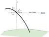Fig. 3 Cartoon showing the loop, the transverse and longitudinal velocities of the waves, and their combination into the observed velocity.

But this cannot be the explanation for the more common edge dislocations observed. We return to the general expression of Eq. (3), and we see that if f(r,θ) is complex, the condition of zero amplitude translates into both the real and imaginary parts being zero independently. If we require a dislocation to be localized in two coordinates, like z and t, both the imaginary and real parts have to depend on them. The interference of two waves with similar wavenumber and/or frequency allows us to introduce an imaginary term ig(r,θ)(−Δkz + Δωt) to the complex amplitude of the wave, but not to the real part. We end up therefore with either just one coordinate fixed for the dislocation or with a linear relationship between both, as we saw, but not with a complete determination of both coordinates. To achieve this we need for the condition on the cancellation of the real part of the complex amplitude to involve z, t, or both. In the interference of the two waves proposed in this section, the other vanishing condition reads as

$\mathit{f}\mathrm{\left(}\mathit{r,\theta }\mathrm{\right)}\mathrm{+}\mathit{g}\mathrm{\left(}\mathit{r,\theta }\mathrm{\right)}\mathrm{=}\mathrm{0}\mathit{,}$which does not depend on either z or t. The scenario of two interfering waves can at most explain one kind of observed dislocation, the gliding edge, but not the most common one, the edge dislocation, in the observations of Fig. 2.

4. Simulating observed dislocations

Since magnetoacoustic waves with different velocities could explain gliding dislocations, we continue exploring this scenario of wave mixing. We now need to consider the fact, already mentioned, that the observed velocity is not necessarily the transverse velocity, but the combination of the projection of both the longitudinal and the transverse velocities on the line of sight, since the loop is not on the plane of the sky (see cartoon in Fig. 3). In the case of Alfvén waves, this makes no difference since the Alfvén wave has no longitudinal velocity component. But magnetoacoustic waves do have a longitudinal velocity component. If the angle of projection is μ, the appropriate velocity projected along the line of sight and observed in Fig. 2 is

${\mathit{v}}_{\mathrm{los}}\mathrm{=}{\mathit{v}}_{\mathrm{long}}\sin \mathit{\mu }\mathrm{\left(}\mathit{z}\mathrm{\right)}\mathrm{-}{\mathit{v}}_{\mathrm{trans}}\cos \mathit{\mu }\mathrm{\left(}\mathit{z}\mathrm{\right)}$where v_trans is already the appropriate projection by the azimuthal angle, a projection to which we should come back later. In that expression, we already made a crucial change: the angle μ will change as we move along the coronal loop, since the loop is roughly a semi-circle starting and ending in the solar photosphere. Therefore there is the potential of finding a dislocation at a given z just because the projection angle μ(z) is the appropriate one at that point. We could develop the conditions for such a dislocation to appear, but we instead notice first that this would give us a dislocation at a given z for all times, something that is not observed. Our next goal is to find a dislocation at fixed z and t. Our solution is to mix the two mechanisms just proposed: the projection of the velocity over the line of sight that fixes z and two waves propagating simultaneously but with different frequencies, which fixes t of the dislocation. Those two simultaneously propagating waves are seen at a projection angle μ(z), so let us compute what would be seen.

A first attempt can be made with two waves having the same value of m. This does not work. No dislocation can be observed in this configuration. The second attempt concerns two waves with different values of m. This was already suggested by López Ariste et al. (2013) as a means to produce observed dislocations. We first suppose that both waves are magnetoacoustic ones. We can suppose here a mode with m = 1, a kink, superposed with a mode with m = 0, a sausage. This comes in handy because the dispersion relations (Edwin & Roberts 1983) show that these two modes propagate at different speeds and frequencies. The simultaneous existence of a sausage and a kink mode in the presence of a coronal density tube will imply that either the tube has a large enough radius or that the sausage mode is a slow mode, two alternatives we return to later.

To proceed with our description, we need to have explicit expressions for the velocities of those wave modes. To write them we use a simple model of a coronal loop formed by a uniform cylindric tube of plasma with piece-wise constant density. In the interior of that cylinder, the magnetoacoustic kink mode can be written as 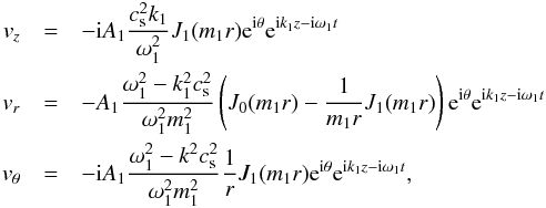$\begin{array}{ccc}{\mathit{v}}_{\mathit{z}}& \mathrm{=}& \mathrm{-}\mathrm{i}{\mathit{A}}_{\mathrm{1}}\frac{{\mathit{c}}_{\mathrm{s}}^{\mathrm{2}}{\mathit{k}}_{\mathrm{1}}}{{\mathit{\omega }}_{\mathrm{1}}^{\mathrm{2}}}{\mathit{J}}_{\mathrm{1}}\mathrm{\left(}{\mathit{m}}_{\mathrm{1}}\mathit{r}\mathrm{\right)}{\mathrm{e}}^{\mathrm{i}\mathit{\theta }}{\mathrm{e}}^{\mathrm{i}{\mathit{k}}_{\mathrm{1}}\mathit{z}\mathrm{-}\mathrm{i}{\mathit{\omega }}_{\mathrm{1}}\mathit{t}}\\ {\mathit{v}}_{\mathit{r}}& \mathrm{=}& \mathrm{-}{\mathit{A}}_{\mathrm{1}}\frac{{\mathit{\omega }}_{\mathrm{1}}^{\mathrm{2}}\mathrm{-}{\mathit{k}}_{\mathrm{1}}^{\mathrm{2}}{\mathit{c}}_{\mathrm{s}}^{\mathrm{2}}}{{\mathit{\omega }}_{\mathrm{1}}^{\mathrm{2}}{\mathit{m}}_{\mathrm{1}}^{\mathrm{2}}}\left({\mathit{J}}_{\mathrm{0}}\mathrm{\left(}{\mathit{m}}_{\mathrm{1}}\mathit{r}\mathrm{\right)}\mathrm{-}\frac{\mathrm{1}}{{\mathit{m}}_{\mathrm{1}}\mathit{r}}{\mathit{J}}_{\mathrm{1}}\mathrm{\left(}{\mathit{m}}_{\mathrm{1}}\mathit{r}\mathrm{\right)}\right){\mathrm{e}}^{\mathrm{i}\mathit{\theta }}{\mathrm{e}}^{\mathrm{i}{\mathit{k}}_{\mathrm{1}}\mathit{z}\mathrm{-}\mathrm{i}{\mathit{\omega }}_{\mathrm{1}}\mathit{t}}\\ {\mathit{v}}_{\mathit{\theta }}& \mathrm{=}& \end{array}$(7)where m₁ is the m₀ defined by Edwin & Roberts (1983) for the case of the kink mode frequency and wavenumber. Always using the same loop model and a similar redefinition of m₀, the magnetoacoustic sausage (m = 0) mode can be written as 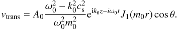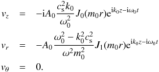$\begin{array}{ccc}{\mathit{v}}_{\mathit{z}}& \mathrm{=}& \mathrm{-}\mathrm{i}{\mathit{A}}_{\mathrm{0}}\frac{{\mathit{c}}_{\mathrm{s}}^{\mathrm{2}}{\mathit{k}}_{\mathrm{0}}}{{\mathit{\omega }}_{\mathrm{0}}^{\mathrm{2}}}{\mathit{J}}_{\mathrm{0}}\mathrm{\left(}{\mathit{m}}_{\mathrm{0}}\mathit{r}\mathrm{\right)}{\mathrm{e}}^{\mathrm{i}{\mathit{k}}_{\mathrm{0}}\mathit{z}\mathrm{-}\mathrm{i}{\mathit{\omega }}_{\mathrm{0}}\mathit{t}}\\ {\mathit{v}}_{\mathit{r}}& \mathrm{=}& \mathrm{-}{\mathit{A}}_{\mathrm{0}}\frac{{\mathit{\omega }}_{\mathrm{0}}^{\mathrm{2}}\mathrm{-}{\mathit{k}}_{\mathrm{0}}^{\mathrm{2}}{\mathit{c}}_{\mathrm{s}}^{\mathrm{2}}}{{\mathit{\omega }}^{\mathrm{2}}{\mathit{m}}_{\mathrm{0}}^{\mathrm{2}}}{\mathit{J}}_{\mathrm{1}}\mathrm{\left(}{\mathit{m}}_{\mathrm{0}}\mathit{r}\mathrm{\right)}{\mathrm{e}}^{\mathrm{i}{\mathit{k}}_{\mathrm{0}}\mathit{z}\mathrm{-}\mathrm{i}{\mathit{\omega }}_{\mathrm{0}}\mathit{t}}\\ {\mathit{v}}_{\mathit{\theta }}& \mathrm{=}& \end{array}$(8)The transverse velocity in both cases still has to be projected onto the plane that contains the line of sight and the z direction. For this we first have to define the direction θ = 0. Without loss of generality, we set this direction along the line of sight. This choice simplifies the expressions above, and for the magnetoacoustic kink, we can write $\begin{array}{ccc}{\mathit{v}}_{\mathrm{trans}}& \mathrm{=}& {\mathit{A}}_{\mathrm{1}}\frac{{\mathit{\omega }}_{\mathrm{1}}^{\mathrm{2}}\mathrm{-}{\mathit{k}}_{\mathrm{1}}^{\mathrm{2}}{\mathit{c}}_{\mathrm{s}}^{\mathrm{2}}}{{\mathit{\omega }}_{\mathrm{1}}^{\mathrm{2}}{\mathit{m}}_{\mathrm{1}}^{\mathrm{2}}}{\mathrm{e}}^{\mathrm{i}{\mathit{k}}_{\mathrm{1}}\mathit{z}\mathrm{-}\mathrm{i}{\mathit{\omega }}_{\mathrm{1}}\mathit{t}}[\mathrm{-}{\mathit{m}}_{\mathrm{1}}{\mathit{J}}_{\mathrm{0}}\mathrm{\left(}{\mathit{m}}_{\mathrm{1}}\mathit{r}\mathrm{\right)}\mathrm{(}{\cos }^{\mathrm{2}}\mathit{\theta }\mathrm{+}\mathit{i}\sin \mathit{\theta }\cos \mathit{\theta }\mathrm{)}\\ & & \mathrm{+}\frac{\mathrm{1}}{\mathit{r}}{\mathit{J}}_{\mathrm{1}}\mathrm{\left(}{\mathit{m}}_{\mathrm{1}}\mathit{r}\mathrm{\right)}\mathrm{(}\cos \mathrm{2}\mathit{\theta }\mathrm{+}\mathrm{i}\sin \mathrm{2}\mathit{\theta }\mathrm{)}]\end{array}$while in the case of the magnetoacoustic sausage, the transverse velocity is just

${\mathit{v}}_{\mathrm{trans}}\mathrm{=}{\mathit{A}}_{\mathrm{0}}\frac{{\mathit{\omega }}_{\mathrm{0}}^{\mathrm{2}}\mathrm{-}{\mathit{k}}_{\mathrm{0}}^{\mathrm{2}}{\mathit{c}}_{\mathrm{s}}^{\mathrm{2}}}{{\mathit{\omega }}_{\mathrm{0}}^{\mathrm{2}}{\mathit{m}}_{\mathrm{0}}^{\mathrm{2}}}{\mathrm{e}}^{\mathrm{i}{\mathit{k}}_{\mathrm{0}}\mathit{z}\mathrm{-}\mathit{i}{\mathit{\omega }}_{\mathrm{0}}\mathit{t}}{\mathit{J}}_{\mathrm{1}}\mathrm{\left(}{\mathit{m}}_{\mathrm{0}}\mathit{r}\mathrm{\right)}\cos \mathit{\theta }\mathit{.}$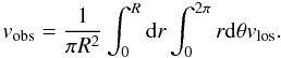Before combining the transverse and longitudinal components projected onto the line of sight for both modes, and to reduce the number of long intermediate expressions, we introduce the last ingredient in our model. The interference of two waves with different frequencies fixes the time that the dislocation occurs. The position z of the dislocation is given by the position along the loop at which the longitudinal and the transverse components of both wave modes are projected with the right angle. But, with the expressions we have at hand at this point, we realize that diferent points in the plane (r,θ) place the dislocation at different values of z and t. To find a dislocation at z and t independently of r and θ, we assume that the cross-section of the coronal loop is smaller than the spatial resolution of the CoMP instrument. Coronal loops are mostly unresolved with current instruments and are certainly so with CoMP. We therefore assume that the full transverse plane (r,θ) of the wave is contained in one pixel, that is, that the radius R of the coronal tube is smaller than the pixel, and this forces us to integrate the velocities in both variables r and θ:

${\mathit{v}}_{\mathrm{obs}}\mathrm{=}\frac{\mathrm{1}}{\mathit{\pi }{\mathit{R}}^{\mathrm{2}}}{\mathrm{\int }}_{\mathrm{0}}^{\mathit{R}}\mathrm{d}\mathit{r}{\mathrm{\int }}_{\mathrm{0}}^{\mathrm{2}\mathit{\pi }}\mathit{r}\mathrm{d}\mathit{\theta }{\mathit{v}}_{\mathrm{los}}\mathit{.}$The integral in θ is particularly interesting since it cancels out most of the terms in the expressions of the velocity, symmetric in azimuth. This cancellation of unresolved velocities has also been pointed out as a concern for observing pure Alfvén waves with m = 0, which are torsional azimuthally symmetric waves. While the sausage mode has to be magnetoacoustic, we notice at this point that the kink mode could either be magnetoacoustic or Alfvén, with both cases resulting in a non-zero transverse velocity after integration on r and θ. In what follows, we continue the calculations for the magnetoacoustic kink mode, keeping in mind that the magnetoacoustic sausage mode could also be interferring with an Alfvén kink mode.

After integration on r and θ, the observed velocity from the magnetoacoustic kink mode, with both the longitudinal and the transverse velocities combined, is 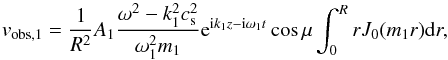${\mathit{v}}_{\mathrm{obs}\mathit{,}\mathrm{1}}\mathrm{=}\frac{\mathrm{1}}{{\mathit{R}}^{\mathrm{2}}}{\mathit{A}}_{\mathrm{1}}\frac{{\mathit{\omega }}^{\mathrm{2}}\mathrm{-}{\mathit{k}}_{\mathrm{1}}^{\mathrm{2}}{\mathit{c}}_{\mathrm{s}}^{\mathrm{2}}}{{\mathit{\omega }}_{\mathrm{1}}^{\mathrm{2}}{\mathit{m}}_{\mathrm{1}}}{\mathrm{e}}^{\mathrm{i}{\mathit{k}}_{\mathrm{1}}\mathit{z}\mathrm{-}\mathrm{i}{\mathit{\omega }}_{\mathrm{1}}\mathit{t}}\cos \mathit{\mu }{\mathrm{\int }}_{\mathrm{0}}^{\mathit{R}}\mathit{r}{\mathit{J}}_{\mathrm{0}}\mathrm{\left(}{\mathit{m}}_{\mathrm{1}}\mathit{r}\mathrm{\right)}\mathrm{d}\mathit{r,}$(9)while the sausage mode is seen as 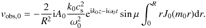${\mathit{v}}_{\mathrm{obs}\mathit{,}\mathrm{0}}\mathrm{=}\mathrm{-}\frac{\mathrm{2}}{{\mathit{R}}^{\mathrm{2}}}\mathrm{i}{\mathit{A}}_{\mathrm{0}}\frac{{\mathit{k}}_{\mathrm{0}}{\mathit{c}}_{\mathrm{s}}^{\mathrm{2}}}{{\mathit{\omega }}_{\mathrm{0}}^{\mathrm{2}}}{\mathrm{e}}^{\mathrm{i}{\mathit{k}}_{\mathrm{0}}\mathit{z}\mathrm{-}\mathrm{i}{\mathit{\omega }}_{\mathrm{0}}\mathit{t}}\sin \mathit{\mu }{\mathrm{\int }}_{\mathrm{0}}^{\mathit{R}}\mathit{r}{\mathit{J}}_{\mathrm{0}}\mathrm{\left(}{\mathit{m}}_{\mathrm{0}}\mathit{r}\mathrm{\right)}\mathrm{d}\mathit{r}\mathit{.}$(10)Finally, to combine the two waves, we rewrite ω = ω₁ and ω₀ = ω₁ + Δω. For simplicity, we assume that k₀ = k₁ = k, since this does not alter the results. Following our model, the observed velocity will be $\begin{array}{ccc}{\mathit{v}}_{\mathit{obs}}& \mathrm{=}& {\mathrm{e}}^{\mathrm{i}\mathit{kz}\mathrm{-}\mathrm{i}{\mathit{\omega }}_{\mathrm{0}}\mathit{t}}\frac{\mathrm{1}}{{\mathit{R}}^{\mathrm{2}}}[\frac{{\mathit{\omega }}^{\mathrm{2}}\mathrm{-}{\mathit{k}}^{\mathrm{2}}{\mathit{c}}_{\mathrm{s}}^{\mathrm{2}}}{{\mathit{\omega }}^{\mathrm{2}}{\mathit{m}}_{\mathrm{1}}}{\mathit{A}}_{\mathrm{1}}\cos \mathit{\mu }{\mathrm{\int }}_{\mathrm{0}}^{\mathit{R}}\mathit{r}{\mathit{J}}_{\mathrm{0}}\mathrm{\left(}{\mathit{m}}_{\mathrm{1}}\mathit{r}\mathrm{\right)}\mathrm{d}\mathit{r}\\ & & \mathrm{-}\mathrm{2}\mathit{i}\frac{\mathit{k}{\mathit{c}}_{\mathrm{s}}^{\mathrm{2}}}{\mathrm{(}\mathit{\omega }\mathrm{+}\mathrm{\Delta }\mathit{\omega }{\mathrm{)}}^{\mathrm{2}}}{\mathit{A}}_{\mathrm{0}}\sin \mathit{\mu }\cos \mathrm{\Delta }\mathit{\omega t}{\mathrm{\int }}_{\mathrm{0}}^{\mathit{R}}\mathit{r}{\mathit{J}}_{\mathrm{0}}\mathrm{\left(}{\mathit{m}}_{\mathrm{0}}\mathit{r}\mathrm{\right)}\mathrm{d}{\mathit{r}}^{}\\ & & \mathrm{+}\mathrm{2}\frac{\mathit{k}{\mathit{c}}_{\mathrm{s}}^{\mathrm{2}}}{\mathrm{(}\mathit{\omega }\mathrm{+}\mathrm{\Delta }\mathit{\omega }{\mathrm{)}}^{\mathrm{2}}}{\mathit{A}}_{\mathrm{0}}\sin \mathit{\mu }\sin \mathrm{\Delta }\mathit{\omega t}{\mathrm{\int }}_{\mathrm{0}}^{\mathit{R}}\mathit{r}{\mathit{J}}_{\mathrm{0}}\mathrm{\left(}{\mathit{m}}_{\mathrm{0}}\mathit{r}\mathrm{\right)}\mathrm{d}\mathit{r}]\mathit{.}\end{array}$(11)This observed velocity wave will show a dislocation when both the imaginary and real parts of the amplitude are simultaneously zero. This leads to the following two equations $\begin{array}{ccc}& & \frac{{\mathit{\omega }}^{\mathrm{2}}\mathrm{-}{\mathit{k}}^{\mathrm{2}}{\mathit{c}}_{\mathrm{s}}^{\mathrm{2}}}{{\mathit{\omega }}^{\mathrm{2}}{\mathit{m}}_{\mathrm{1}}}{\mathit{A}}_{\mathrm{1}}\cos \mathit{\mu }{\mathrm{\int }}_{\mathrm{0}}^{\mathit{R}}\mathit{r}{\mathit{J}}_{\mathrm{0}}\mathrm{\left(}{\mathit{m}}_{\mathrm{1}}\mathit{r}\mathrm{\right)}\mathrm{d}\mathit{r}\\ & & \mathrm{+}\mathrm{2}\frac{\mathit{k}{\mathit{c}}_{\mathrm{s}}^{\mathrm{2}}}{\mathrm{(}\mathit{\omega }\mathrm{+}\mathrm{\Delta }\mathit{\omega }{\mathrm{)}}^{\mathrm{2}}}{\mathit{A}}_{\mathrm{0}}\sin \mathit{\mu }\sin \mathrm{\Delta }\mathit{\omega t}{\mathrm{\int }}_{\mathrm{0}}^{\mathit{R}}\mathit{r}{\mathit{J}}_{\mathrm{0}}\mathrm{\left(}{\mathit{m}}_{\mathrm{0}}\mathit{r}\mathrm{\right)}\mathrm{d}\mathit{r}\mathrm{=}\mathrm{0}\\ & & \frac{\mathit{k}{\mathit{c}}_{\mathrm{s}}^{\mathrm{2}}}{\mathrm{(}\mathit{\omega }\mathrm{+}\mathrm{\Delta }\mathit{\omega }{\mathrm{)}}^{\mathrm{2}}}\sin \mathit{\mu }\cos \mathrm{\Delta }\mathit{\omega t}\mathrm{=}\mathrm{0.}\end{array}$The second of these two conditions implies that, other than the trivial case μ = 0, the observed velocity will present a dislocation only if

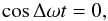$\cos \mathrm{\Delta }\mathit{\omega t}\mathrm{=}\mathrm{0}\mathit{,}$that is, at those times when the two waves are in anti-phase¹. This fixes, as expected, a time t when the dislocation is possible depending on the difference in frequency and on the precise moment when either wave was excited at, let us say, the feet of the loop. It is interesting to notice that, given the wavelength of the coronal waves, one does not expect this cophasing to happen more than once per loop. By inserting this cophasing condition in the first condition for the dislocation, we obtain a formula for the angle μ at which such dislocation would be visible: 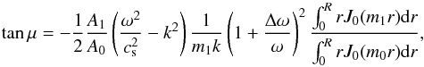$\tan \mathit{\mu }\mathrm{=}\mathrm{-}\frac{\mathrm{1}}{\mathrm{2}}\frac{{\mathit{A}}_{\mathrm{1}}}{{\mathit{A}}_{\mathrm{0}}}\left(\frac{{\mathit{\omega }}^{\mathrm{2}}}{{\mathit{c}}_{\mathrm{s}}^{\mathrm{2}}}\mathrm{-}{\mathit{k}}^{\mathrm{2}}\right)\frac{\mathrm{1}}{{\mathit{m}}_{\mathrm{1}}\mathit{k}}{\left(\mathrm{1}\mathrm{+}\frac{\mathrm{\Delta }\mathit{\omega }}{\mathit{\omega }}\right)}^{\mathrm{2}}\frac{{\mathrm{\int }}_{\mathrm{0}}^{\mathit{R}}\mathit{r}{\mathit{J}}_{\mathrm{0}}\mathrm{\left(}{\mathit{m}}_{\mathrm{1}}\mathit{r}\mathrm{\right)}\mathrm{d}\mathit{r}}{{\mathrm{\int }}_{\mathrm{0}}^{\mathit{R}}\mathit{r}{\mathit{J}}_{\mathrm{0}}\mathrm{\left(}{\mathit{m}}_{\mathrm{0}}\mathit{r}\mathrm{\right)}\mathrm{d}\mathit{r}}\mathit{,}$(14)with an equivalent formula for the case of an Alfvén kink wave interfering with the magnetoacoustic sausage mode.

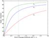Fig. 4 Angle μ at which the dislocation will be seen following Eq. (14) for different velocities of the magnetoacoustic kink wave, assuming a sound speed cs = 100 km s-1, an Alfvén speed 10 times the speed of sound, a period of 3 min for the kink wave, and a 5% difference in frequency between the kink and the sausage waves.

A dislocation will be seen at time t at the position z where the two waves happen to be in phase and which is seen by the observer at an angle μ given by Eq. (14). Figure 4 shows examples of the variation of the angle μ with the ratio of amplitudes for three different values of the phase speed of the magnetoacoustic kink wave. It has been computed for typical values of the sound and Alfvén speed in the corona (100 and 1000 km s^-1, respectively) for an average wave period of three minutes and a 5% difference in frequency between the two waves. As an example of what would be seen, we show in Fig. 5 the observed Doppler velocity for the case of a fast kink wave propagating at seven times the speed of sound (700 km s^-1), interfering with a slow sausage wave, which presents a ratio of amplitudes $\frac{{\mathit{A}}_{\mathrm{1}}}{{\mathit{A}}_{\mathrm{0}}}\mathrm{=}\mathrm{0.25}$. These are the scalar amplitudes of the full vector wave or, in other words, the amplitudes of the pressure wave. The observed velocities have amplitudes given by these A₁ and A₀ times other factors (see Eqs. (7) and (8)), resulting in the kink velocity having a larger amplitude than the sausage velocity even if A₁ is smaller than A₀. With these numbers, as expected, a dislocation appears at roughly μ = 50°. The result is visually striking as a correct reproduction of the edge dislocations observed in coronal waves by CoMP and seen in Fig. 2.

If sausage and kink waves were excited in perfect phase matching at the loop feet, the dislocation would be visible periodically at most at one position along the loop (with a very long period $\mathit{P}\mathrm{=}\frac{\mathrm{2}\mathit{\pi }}{\mathrm{\Delta }\mathit{\omega }}$). The observed changes in position and time mean that the conditions of excitation of kinks and sausages in the loop feet vary permanently. If the kink wave propagated at roughly the speed of sound, the factor $\frac{{\mathit{\omega }}^{\mathrm{2}}}{{\mathit{c}}_{\mathrm{s}}^{\mathrm{2}}}\mathrm{-}{\mathit{k}}_{\mathrm{1}}^{\mathrm{2}}$ would be zero and the dislocation would only be found at low values of z. This is not the case: dislocations are seen for all values of z in Fig. 2. From this we have to conclude that the kink mode is either an Alfvén mode or a fast wave moving at speeds comparable to the Alfvén speed.

If the sausage mode is a slow mode, which can propagate independently of the radius of the loop, then it is easy to imagine that the dislocation arises from the excitation of a kink mode, Alfvén or magnetoacoustic, that propagates at high speed along the loop and catches up with a sausage slow mode excited some time earlier. When this happens will depend on their respective velocities, but also on the time between both excitations. Where this happens (if visible) will depend on the respective velocities, but also on the ratio of amplitudes of both waves. Threlfall et al. (2013) measured a phase speed around 700 km s^-1, roughly corresponding to seven times the speed of sound. We see that at this high speed, the spread of dislocations observed in Fig. 2 translates into magnetoacoustic kink amplitudes smaller than the sausage ones, although with a preference for dislocations concentrating in the top part of the loop. This appears to be the case in Fig. 2.

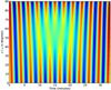Fig. 5 Simulation of an observation of magnetoacoustic kink and sausage modes propagating along a circular loop with a 5% difference in frequency, at a ratio of 7 in phase speeds and a ratio of amplitudes $\frac{{\mathit{A}}_{\mathrm{1}}}{{\mathit{A}}_{\mathrm{0}}}\mathrm{=}\mathrm{0.25}$. The z coordinate along the loop is given in terms of the angle μ it forms with the line of sight at each point.

5. Discussion

Observations of waves in the Doppler measurements of coronal emission lines by CoMP show wavefront dislocations. Several qualitative and quantitative arguments were made to ensure this identification of the wave singularity in the observed data. The conclusive identification of these singularities called dislocations requires an explanation in terms of the waves expected to propagate in those coronal regions and their velocities projected along the line of sight, seen as Doppler shifts in the coronal emission lines observed by CoMP.

We have provided such an explanation while explicitly discarding several other possibilities. We recall that the observations were projected in a diagram z−t where z was the direction of propagation of the waves, also assumed to be the direction of the magnetic field. The dislocations were mostly of the edge type, meaning that the phase singularity was found at isolated points in the z−t plane. The waves naturally propagating along the magnetic field in the corona carry dislocations, but those dislocations are of the edge type only on the plane transverse to z, which in cylindric coordinates we can refer to as the plane r−θ. These basic dislocations carried by the waves propagating along the magnetic field in coronal conditions cannot explain the observations. Our first conclusion in this paper is therefore that the observations cannot be explained by single propagating waves of one type or the other: the presence of dislocations forces us to look for more elaborated scenarios of propagating waves.

Three ingredients are needed to fix the dislocation in one single point of the z−t diagram as observed. First, the interference of two waves with different frequencies can fix the dislocation in time, but not in z. Second, the combination of transverse and longitudinal velocity components by projection onto the line of sight, can fix the dislocation in z but not in time, as long as the transverse and longitudinal components belong to waves of different modes m (sausage and kink waves, for example). Furthermore, the position z of the dislocation varies for different points in the transverse plane r−θ. Third, the integration of the line emission over the transverse plane r−θ allows fixing a single z and t for the whole emitting region with two interfering waves at different frequencies, if that transverse section of the loop is not spatially resolved.

In our analysis, we used a very simple model for a coronal loop and the propagation of waves along it. When adding in particular non-homogeneous density profiles across the loop rather than the piecewise-constant density we used, more sophisticated or realistic models will still conserve the azimuthal symmetries in the solutions to the propagating modes that are at the core of our explanation of the observed dislocations. The actual details of the solution, the radial dependencies in terms of Bessel functions or others, and the distribution of visible dislocations along the loop, all those aspects may change in those more realistic models. It is disturbing that, for example, when the density is allowed to vary in a continuous manner, the classic kink wave becomes a surface Alfvén wave with a strong Alfvénic character Goossens et al. (2009, 2012), and the solutions display rapid variations in the radial and azimuthal components at the resonant layer with the consequence that the global motion is quickly damped. It is difficult to foresee what the consequences would be for the existence and properties of dislocations as described in this study. But we are confident that the need for interference of two modes with different azimuthal number m at slightly different frequencies with longitudinal and transverse velocities combined in the projection onto the line of sight will still be the ingredients that explain the observed dislocations. Simpler conditions do not seem to work, and more complicated ones may not be very common and harder to be simultaneously met.

Indeed, we appreciate in our explanation that the three ingredients (interference of waves of different frequency, combination of longitudinal and transverse velocity components into the line of sight, and integration of the full emitting region inside the pixel) are quite natural and common. It is not surprising therefore that the observations show a large number of dislocations during the observation. But the same three ingredients also limit the type of waves responsible for the observations. Thus the integration over the r−θ plane excludes from the model any wave with azimuthal symmetry. Pure Alfvén waves with m = 0, in particular, result in a zero signal and can be excluded.

The need for a longitudinal velocity component implies the presence of at least one magnetoacoustic wave. Sausage modes (m = 0) can be responsible of the longitudinal velocity component, but their transverse velocity is azimuthally symmetric and cancels out. Kink waves (m = 1), either magnetoacoustic or Alfvén, can be responsible of the transverse velocity component, but not of the longitudinal one, in one case because it cancels out and in the other, because there is no longitudinal component.

All conditions are satisfied when we consider the addition of magnetoacoustic sausage and a kink wave (either magnetoacoustic or Alfvén) having slightly different frequencies. Integrated across the loop, the observed Doppler shift is made of the transverse velocity of the kink mode plus the longitudinal velocity of the sausage mode. At those points along the loop with the right projection angle, the interference of the two waves with the right phases results in a dislocation localized in z−t as observed. The equation for the appearance of the dislocation also suggests that, at high speeds of the kink wave, dislocations will be more frequently observed on the top of the loops, but some variability in position is expected if the amplitude of the kink mode is smaller than that of the sausage mode.

All this appears to be the case in the solar corona, leading us to conclude that a fast kink mode, either a fast magnetoacoustic or an Alfvén one, catches up to a slow sausage mode at some point along the loop and produces a dislocation visible with COMP. The fast character of the kink mode is suggested by the measured speed of the observed wave (Threlfall et al. 2013), but also by the comparison of the predictions of Fig. 4 with the observed positions of the dislocations in Fig. 2. The slow character of the sausage mode makes it compatible with a propagation with cross-sections smaller than CoMP spatial resolutions that justify our integration in r and θ, and apparently smaller than the cutoff of fast sausage modes. A slow sausage mode also makes it a good candidate for being over-run often by fast and/or Alfvén kink modes excited at different times.

Threlfall et al. (2013) compared the observed waves in CoMP with simultaneous observations of emission, hence density, perturbations observed by AIA. The density perturbation corresponding to our two waves is ${\mathit{\rho }}_{\mathrm{1}}\mathrm{=}\mathrm{-}\mathrm{i}{\mathit{A}}_{\mathrm{0}}\frac{{\mathit{\rho }}_{\mathrm{0}}}{\mathit{\omega }}{\mathit{J}}_{\mathit{m}}\mathrm{\left(}{\mathit{m}}_{\mathrm{0}}\mathit{r}\mathrm{\right)}{\mathrm{e}}^{\mathrm{i}\mathit{kz}\mathrm{-}\mathrm{i}\mathit{\omega t}}\mathit{.}$(15)Despite the absence of any azimuthal dependence, the radial integral of the J₁(m₀r) in the case of a fast magnetoacoustic kink is going to be almost negligible compared to the same integral of the J₀(m₀r) function for the slow sausage mode. The compressional wave will therefore be dominated by the sausage mode. The Doppler signal, on the other hand, will be dominated by the kink mode. As a result, the two instruments are sensitive to one or the other wave but not to both, and one should not expect any spatial correlation between observations of the compression wave by AIA/SDO and observations of the velocity wave by COMP. In spite of this, the observed periods (frequencies) will of course be similar. This coincides with the conclusions of Threlfall et al. (2013).

6. Conclusion

We have identified wavefront dislocations in the observations of coronal waves made by CoMP. Explaining the observed dislocations forced us to abandon the image of a single wave propagating in those coronal structures. We explain in detail the only scenario we have found that can explain the observations. Our model is made of two propagating waves that have different wave frequencies and are in interference. The two waves have different azimuth dependences (or charges), and the observations integrate the velocity wave over the full cross-section of the wave, which is smaller than the spatial resolution of the instrument. This eliminates many possible candidates for which the signals cancel out after integration. In particular, torsional Alfvén waves with m = 0 are excluded, but magnetoacoustic sausage waves appear to a necessity, combined with a kink mode that can be either a fast magnetoacoustic mode or an Alfvén wave. The two wave modes, the magnetoacoustic sausage and the kink, propagating at different frequencies and integrated over the loop cross-section are seen under different projection angles at different positions along the loop. This projection of the transverse and longitudinal velocities of the two waves onto the line-of-sight fixes when and where the dislocation will be seen.

Computing these conditions for the visibility of the dislocations leads us to conclude that our model can reproduce the observations if we assume a fast kink mode (magnetoacoustic or Alfvén) that catches up over a slow sausage mode propagating along the coronal loop. The observed signature is dominated by the velocity amplitude of the fast kink mode, although the pressure amplitude of the slow sausage is still larger than that of the kink mode. Following our model, the observed dislocations also imply that the spatial resolution of the observations is not high enough to resolve the cross-section of the loop: we see an integrated signal. Despite the simplified model used for our analysis, the conditions under which dislocations can be seen in the data appear quite general and translatable to more sophisticated models.

The sausage modes required in our scenario to explain the dislocation may coincide with the density waves observed by AIA/SDO (Threlfall et al. 2013). The density perturbation in our model is dominated by the sausage mode, even if the kink mode is magnetoacoustic. Observations of emission changes, mostly proportional to the density, would then mostly see this mode rather than the kink one. Although of similar frequency and period, the very different wavelengths will make them difficult to correlate with the observed velocity wave, which is mostly dominated by the kink mode.

Finally, we insist that the observations cannot be explained by Alfvén waves alone, but instead require a combination of at least one magnetoacoustic mode. The relative amplitude of these modes will have to be explained by the excitation of these waves or its propagation and eventual dissipation in the low parts of the corona. The existence of other propagating modes cannot be fully discarded, but since they cannot be responsible for the observations due, as for the case of the torsional Alfvén wave, to their azimuthal symmetries, they have to be considered as unobserved or irrelevant for the present observations. On the other hand, the continuous existence and interaction of two waves must be seen as a permanent feature of coronal loops.

Online material

Appendix A: Direct computation of the monodromy

In the main body of this paper, we computed the monodromy through the trick of identifying places of known phase in the data and drawing the closed curve through those places. We drew lines along contiguous places of known phase in the crests or the valleys of the waves on both sides of the suspected dislocation and joined them with a straight line that crossed an integer amount of the crests or valleys. This method was suggested by the organized patterns in the data that allowed an easy and safe identification of those places of known phase. But to feel fully confident about the method and the presence of the dislocation, we would prefer to be able to directly solve the monodromy integral along any closed curve in a general wave field.

The observed data in our present case is the Doppler shift of an emission line interpreted as the line-of-sight velocity of the plasma. This is a real quantity. Our first step will be to interpret these observations as the real part of a complex wave field for which we have to determine the imaginary part. For simplicity we assume that the observation can be safely interpreted as due to a wave with a unique average frequency ω. We can describe the observed wave field as

$\mathit{\phi }\mathrm{\left(}\mathit{z,t}\mathrm{\right)}\mathrm{=}\mathit{A}\mathrm{\left(}\mathit{z,t}\mathrm{\right)}\cos (\mathit{\omega t}\mathrm{+}\mathit{\alpha }\mathrm{\left(}\mathit{z,t}\mathrm{\right)}\mathrm{)}\mathit{.}$The observations, which is the real quantity φ at each position (z,t), are described as a variable real amplitude A(z,t) times a cosine variation in time with frequency ω. We asume a constant zero time for the full wave field, but allow for a local phase shift α(z,t) that, through its time dependence, may include local frequency changes. The combination of the variable amplitude and local phase shifts allows describing very complicated wave patterns, including the one in Fig. 2, as long as one accepts the constant average frequency ω over the time and place of the observation.

We can decompose the cosine function as

$\cos \left(\mathit{\omega t}\mathrm{+}\mathit{\alpha }\mathrm{\left(}\mathit{z,t}\mathrm{\right)}\right)\mathrm{=}\cos \mathit{\omega t}\cos \mathit{\alpha }\mathrm{-}\sin \mathit{\omega t}\sin \mathit{\alpha }\mathit{.}$The local phase shift α can now be interpreted as a local modification of the amplitude of two different waves: $\begin{array}{ccc}\mathit{\phi }& \mathrm{=}& \left[\mathit{A}\mathrm{\left(}\mathit{z,t}\mathrm{\right)}\cos \mathit{\alpha }\cos \mathit{\omega t}\right]\mathrm{-}\left[\mathit{A}\mathrm{\left(}\mathit{z,t}\mathrm{\right)}\sin \mathit{\alpha }\sin \mathit{\omega t}\right]\\ & \mathrm{=}& {\mathit{\psi }}_{\mathit{C}}\cos \mathit{\omega t}\mathrm{+}{\mathit{\psi }}_{\mathit{S}}\sin \mathit{\omega t}\mathit{.}\end{array}$This suggests the construction of the complex wave field

$\mathit{\psi }\mathrm{\left(}\mathit{z,t}\mathrm{\right)}\mathrm{=}\mathrm{(}{\mathit{\psi }}_{\mathit{C}}\mathrm{+}\mathrm{i}{\mathit{\psi }}_{\mathit{S}}\mathrm{)}{\mathrm{e}}^{\mathrm{i}\mathit{\omega t}}$This wave has an amplitude

${\mathit{\psi }}_{\mathit{C}}^{\mathrm{2}}\mathrm{+}{\mathit{\psi }}_{\mathit{S}}^{\mathrm{2}}\mathrm{=}{\mathit{A}}^{\mathrm{2}}$which is the amplitude of the observed wave, while locally it adds a phase χ

$\tan \mathit{\chi }\mathrm{=}\frac{{\mathit{\psi }}_{\mathit{S}}}{{\mathit{\psi }}_{\mathit{C}}}\mathrm{=}\frac{\sin \mathit{\alpha }}{\cos \mathit{\alpha }}\mathrm{=}\tan \mathit{\alpha ,}$which is identical to the local phase of the observed wave. Thus the proposed complex wave field

$\mathit{\psi }\mathrm{\left(}\mathit{z,t}\mathrm{\right)}\mathrm{=}\mathit{A}\mathrm{\left(}\mathit{z,t}\mathrm{\right)}{\mathrm{e}}^{\mathrm{i}\mathit{\alpha }\mathrm{\left(}\mathit{z,t}\mathrm{\right)}}{\mathrm{e}}^{\mathrm{i}\mathit{\omega t}}$has the same observable parameters as the original real wave φ(z,t) and can be used instead of it, with a straightforward (diffeomorphic) correspondence between them.

Since z and t are the coordinates of Fig. 2, we rewrite this complex field for the wave on the longitudinal velocity as just a real amplitude and a phase

$\mathit{\psi }\mathrm{\left(}\mathit{z,t}\mathrm{\right)}\mathrm{=}\mathit{\rho }{\mathrm{e}}^{\mathrm{i}\mathit{\chi }}\mathit{.}$After differentiating this expression, we find that 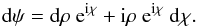$\mathrm{d}\mathit{\psi }\mathrm{=}\mathrm{d}\mathit{\rho }{\mathrm{e}}^{\mathrm{i}\mathit{\chi }}\mathrm{+}\mathrm{i}\mathit{\rho }{\mathrm{e}}^{\mathrm{i}\mathit{\chi }}\mathrm{d}\mathit{\chi }\mathit{.}$(A.1)Dividing by ψ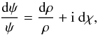$\frac{\mathrm{d}\mathit{\psi }}{\mathit{\psi }}\mathrm{=}\frac{\mathrm{d}\mathit{\rho }}{\mathit{\rho }}\mathrm{+}\mathrm{i}\mathrm{d}\mathit{\chi ,}$(A.2)we can integrate both sides of this last expression along a closed curve C, the monodromy:

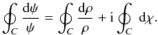${\mathrm{􏽉}}_{\mathit{C}}\frac{\mathrm{d}\mathit{\psi }}{\mathit{\psi }}\mathrm{=}{\mathrm{􏽉}}_{\mathit{C}}\frac{\mathrm{d}\mathit{\rho }}{\mathit{\rho }}\mathrm{+}\mathrm{i}{\mathrm{􏽉}}_{\mathit{C}}\mathrm{d}\mathit{\chi }\mathit{.}$Since ρ, the amplitude of the complex wave, is, by definition, a real quantity, we find that ${{}^{\mathrm{􏽈}}}_{\mathit{C}}\frac{\mathrm{d}\mathit{\rho }}{\mathit{\rho }}\mathrm{=}\mathrm{0}$ on any closed curve, and the monodromy simplifies to 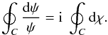${\mathrm{􏽉}}_{\mathit{C}}\frac{\mathrm{d}\mathit{\psi }}{\mathit{\psi }}\mathrm{=}\mathrm{i}{\mathrm{􏽉}}_{\mathit{C}}\mathrm{d}\mathit{\chi }\mathit{.}$(A.3)The righthand part is the monodromy over the phase of the wave, which if different than zero, identifies the presence of a singularity, a dislocation, inside the closed curve. The lefthand part is an integral over the observed data. We conclude that from the observations, we can build a complex field ψ and then compute the integral on the left along the chosen closed path C to obtain the required integral over the phase on the right. This solves the problem of computing the monodromy on the phase directly from the data. It is useful to make one further step. The integral on the lefthand side can be formally integrated $\log \frac{{\mathit{\psi }}_{\mathit{f}}}{{\mathit{\psi }}_{\mathrm{i}}}\mathrm{=}\mathrm{i}{\mathrm{􏽉}}_{\mathit{C}}\mathrm{d}\mathit{\chi ,}$(A.4)where ψ_f and ψ_i are the final and initial values, respectively, of ψ at the closed path. These would be the same, since the path is closed, except that the ψ function is complex. This raises the possibility of those initial and final values not being in the same Riemann surface of the logarithm function. Indeed, the complex logarithm² is log z = (log z)_principal + i2πN. The principal value of the logarithm is identical for the initial and final points, so that we can conclude that ${\mathrm{􏽉}}_{\mathit{C}}\mathrm{d}\mathit{\chi }\mathrm{=}\mathrm{-}\mathrm{2}\mathit{\pi N,}$(A.5)where N is the number of twists made by the logarithm function as it follows the path C.

Acknowledgments

The authors acknowledge financial support from the Spanish Ministry of Economy and Competitiveness (MINECO) AYA2011-24808, AYA2011-22846, and AYA2010-18029, from the Ramón y Cajal fellowship, and from the projects CSD2007-00050 and ERC-2011-StG 277829-SPIA Starting Grant, financed by the European Research Council.

References

All Figures

	Fig. 1 Four examples of dislocations in the propagation of a wave with the time in abscissas and a distance in ordinates. From left to right, a vortex, two edges, and a gliding edge, all with charge 1. Around the second edge dislocation, a closed curve has been drawn with dots and squares. The integral of the phase along this curve, the monodromy, is non-zero.
In the text

Fig. 2 Observation of coronal waves in the Doppler velocity of a coronal emission line by COMP from Threlfall et al. (2013). The diagram has time in abscissas and the coordinate z, along the loop and parallel to the magnetic field, in ordinates. Among the many visible dislocations, two have been labeled. The closed curve (that could represent the monodromy) encloses an edge dislocation, while the straight segment follows a possible gliding dislocation.

In the text

	Fig. 3 Cartoon showing the loop, the transverse and longitudinal velocities of the waves, and their combination into the observed velocity.
In the text

	Fig. 4 Angle μ at which the dislocation will be seen following Eq. (14) for different velocities of the magnetoacoustic kink wave, assuming a sound speed cs = 100 km s-1, an Alfvén speed 10 times the speed of sound, a period of 3 min for the kink wave, and a 5% difference in frequency between the kink and the sausage waves.
In the text

Fig. 5 Simulation of an observation of magnetoacoustic kink and sausage modes propagating along a circular loop with a 5% difference in frequency, at a ratio of 7 in phase speeds and a ratio of amplitudes $\frac{{\mathit{A}}_{\mathrm{1}}}{{\mathit{A}}_{\mathrm{0}}}\mathrm{=}\mathrm{0.25}$. The z coordinate along the loop is given in terms of the angle μ it forms with the line of sight at each point.

In the text

References

- Arregui, I. 2015, Phil. Trans. Roy. Soc. A, 373, 20140261 [Google Scholar]
- Arregui, I., & Asensio Ramos, A. 2011, ApJ, 740, 44 [NASA ADS] [CrossRef] [Google Scholar]
- Arregui, I., Andries, J., Van Doorsselaere, T., Goossens, M., & Poedts, S. 2007, A&A, 463, 333 [NASA ADS] [CrossRef] [EDP Sciences] [Google Scholar]
- Aschwanden, M. J., Fletcher, L., Schrijver, C. J., & Alexander, D. 1999, ApJ, 520, 880 [NASA ADS] [CrossRef] [Google Scholar]
- Centeno, R., Collados, M., & Trujillo Bueno, J. 2006, ApJ, 640, 1153 [NASA ADS] [CrossRef] [PubMed] [Google Scholar]
- Cirtain, J. W., Golub, L., Lundquist, L., et al. 2007, Science, 318, 1580 [NASA ADS] [CrossRef] [PubMed] [Google Scholar]
- De Moortel, I., & Nakariakov, V. M. 2012, Roy. Soc. London Philos. Trans. Ser. A, 370, 3193 [Google Scholar]
- De Pontieu, B., McIntosh, S. W., Carlsson, M., et al. 2007, Science, 318, 1574 [NASA ADS] [CrossRef] [PubMed] [Google Scholar]
- Edwin, P. M., & Roberts, B. 1983, Sol. Phys., 88, 179 [NASA ADS] [CrossRef] [Google Scholar]
- Goossens, M., Arregui, I., Ballester, J. L., & Wang, T. J. 2008, A&A, 484, 851 [NASA ADS] [CrossRef] [EDP Sciences] [Google Scholar]
- Goossens, M., Terradas, J., Andries, J., Arregui, I., & Ballester, J. L. 2009, A&A, 503, 213 [NASA ADS] [CrossRef] [EDP Sciences] [Google Scholar]
- Goossens, M., Andries, J., Soler, R., et al. 2012, ApJ, 753, 111 [NASA ADS] [CrossRef] [Google Scholar]
- Lin, Y., Soler, R., Engvold, O., et al. 2009, ApJ, 704, 870 [NASA ADS] [CrossRef] [Google Scholar]
- López Ariste, A., Collados, M., & Khomenko, E. 2013, Phys. Rev. Lett., 111, 81103 [NASA ADS] [CrossRef] [Google Scholar]
- Nakariakov, V. M., & Ofman, L. 2001, A&A, 372, L53 [NASA ADS] [CrossRef] [EDP Sciences] [Google Scholar]
- Nakariakov, V. M., Ofman, L., Deluca, E. E., Roberts, B., & Davila, J. M. 1999, Science, 285, 862 [NASA ADS] [CrossRef] [PubMed] [Google Scholar]
- Nye, J. F., & Berry, M. V. 1974, Roy. Soc. London Proc. Ser. A, 336, 165 [Google Scholar]
- Okamoto, T. J., Tsuneta, S., Berger, T. E., et al. 2007, Science, 318, 1577 [NASA ADS] [CrossRef] [PubMed] [Google Scholar]
- Parnell, C. E., & De Moortel, I. 2012, Roy. Soc. London Philos. Trans. Ser. A, 370, 3217 [Google Scholar]
- Priest, E. R. 1982, Solar magneto-hydrodynamics (Dordrecht, The Netherlands: D. Reidel Pub. Co.), 23 [Google Scholar]
- Roberts, B. 1981, Sol. Phys., 69, 27 [NASA ADS] [CrossRef] [Google Scholar]
- Spruit, H. C. 1982, Sol. Phys., 75, 3 [NASA ADS] [CrossRef] [Google Scholar]
- Threlfall, J., De Moortel, I., McIntosh, S. W., & Bethge, C. 2013, A&A, 556, A124 [NASA ADS] [CrossRef] [EDP Sciences] [Google Scholar]
- Tomczyk, S., & McIntosh, S. W. 2009, ApJ, 697, 1384 [NASA ADS] [CrossRef] [Google Scholar]
- Tomczyk, S., McIntosh, S. W., Keil, S. L., et al. 2007, Science, 317, 1192 [NASA ADS] [CrossRef] [PubMed] [Google Scholar]
- Tomczyk, S., Card, G. L., Darnell, T., et al. 2008, Sol. Phys., 247, 411 [NASA ADS] [CrossRef] [Google Scholar]
- Wentzel, D. G. 1979, A&A, 76, 20 [NASA ADS] [Google Scholar]