| Issue |
A&A
Volume 578, June 2015
|
|
|---|---|---|
| Article Number | A98 | |
| Number of page(s) | 5 | |
| Section | Interstellar and circumstellar matter | |
| DOI | https://doi.org/10.1051/0004-6361/201526107 | |
| Published online | 11 June 2015 | |
Circumstellar disks revealed by H/K flux variation gradients
1 Astronomisches Institut, Ruhr–Universität Bochum, Universitätsstraße 150, 44801 Bochum, Germany
e-mail: This email address is being protected from spambots. You need JavaScript enabled to view it.
2 Instituto de Astronomía, Universidad Católica del Norte, Avenida Angamos 0610, Casilla 1280 Antofagasta, Chile
3 Institute for Astronomy, University of Hawaii, 640 N. Aohoku Place, Hilo, HI 96720, USA
Received: 16 March 2015
Accepted: 28 April 2015
Abstract
The variability of young stellar objects (YSO) changes their brightness and color preventing a proper classification in traditional color−color and color magnitude diagrams. We have explored the feasibility of the flux variation gradient (FVG) method for YSOs, using H and K band monitoring data of the star forming region RCW 38 obtained at the University Observatory Bochum in Chile. Simultaneous multi-epoch flux measurements follow a linear relation FH = α + β·FK for almost all YSOs with large variability amplitude. The slope β gives the mean HK color temperature Tvar of the varying component. Because Tvar is hotter than the dust sublimation temperature, we have tentatively assigned it to stellar variations. If the gradient does not meet the origin of the flux-flux diagram, an additional non- or less-varying component may be required. If the variability amplitude is larger at the shorter wavelength, e.g. α< 0, this component is cooler than the star (e.g. a circumstellar disk); vice versa, if α> 0, the component is hotter like a scattering halo or even a companion star. We here present examples of two YSOs, where the HK FVG implies the presence of a circumstellar disk; this finding is consistent with additional data at J and L. One YSO shows a clear K-band excess in the JHK color−color diagram, while the significance of a K-excess in the other YSO depends on the measurement epoch. Disentangling the contributions of star and disk it turns out that the two YSOs have huge variability amplitudes (~3−5 mag). The HK FVG analysis is a powerful complementary tool to analyze the varying components of YSOs and worth further exploration of monitoring data at other wavelengths.
Key words: stars: formation / circumstellar matter / stars: individual: RCW38 / stars: variables: general
© ESO, 2015
1. Introduction
The paradigm of a low-mass young stellar object (YSO) involves a pre-main-sequence star surrounded by a circumstellar disk (CSD), a (bi)-polar reflection nebula and an envelope. Establishing the presence of a CSD is an observational challenge.
The classical technique is to reveal the presence of (T ~ 1500 K) dust of the CSD by means of a K-excess in JHK color−color diagrams; the YSO is then located at large H − K values compared to small J − H, i.e. the right hand of the reddening vector (e.g. Meyer et al. 1997). One problem of this technique is to distinguish between the various emission components: star, disk, and a possible reflection nebula. When the CSD is seen nearly edge-on, the star is dimmed and heavily reddened so that the apparent stellar temperature approaches that of the CSD dust. Likewise only a minor contribution from the less reddened reflection nebula may be recognisable. In the JHK diagram such a type-2 YSO will be located at both large J − H and large H − K values, hence only barely distinguishable from highly reddened sources without CSDs (e.g. Kenyon et al. 1993; Stark et al. 2006).
Instead of analyzing multi-component YSOs in magnitude units, it appears more promising to consider flux (density) or energy units. Meanwhile numerous multi-wavelength spectral energy distributions (SEDs) are available, but mostly observed at different epochs; this potentially limits the results of SED analyses in the case of variable objects. However, YSOs in particular undergo strong brightness variations at X-ray, optical, and near-infrared (NIR) wavelengths, for instance owing to stochastic fluctuations of the accretion or to rotating hot/cool spots on the stellar surface.
Therefore, a valuable complement to multi-wavelength SED studies is the variability monitoring of YSOs, preferably in the NIR so as to be less sensitive to extinction. Simultaneous data in two or more filters provide valuable color information. Assuming that the variations originate in the star and not in the circumstellar matter, then – in a given aperture – one measures the superposition of a varying hot stellar component and non-varying cool disk component.
This is exactly the analog of what the two-filter flux variation gradient (FVG) method reveals in Seyfert galaxies: a hot varying nucleus and a cool non-varying contamination by the host galaxy (Choloniewski 1981; Winkler et al. 1992; Glass 2004; Sakata et al. 2010; Haas et al. 2011; Pozo Nuñez et al. 2012, 2013, 2014, 2015). If the central source is sufficiently hot to allow for a Rayleigh-Jeans approximation, the flux is proportional to the temperature, and therefore a linear relation between fluxes from the two filters is expected.
To separate the contributions from variable hot stars and a more constant circumstellar environment, we have explored the capability of the FVG method for YSOs, using H and K band monitoring data of the star forming region RCW 38 obtained at the University Observatory Bochum in Chile. Here, we report on a first feasibility study, with the focus on the linear relationship between the H and K fluxes, and subsequent potential applications.
2. Near-infrared data
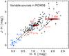 |
Fig. 1 Color−color diagram of variable sources in RCW 38. Black dots with error bars denote averaged photometric single observations from Dörr et al (2013). The main sequence is shown in blue and the locus of unreddened classical T Tauri stars (CTTS) by the red long-dashed line. Two sources with ID 557 and 559 are highlighted in red; the small circles mark the individual H and K measurements placed at mean J − H owing to the lack of J variability data; the large circles give the mean H − K. The AV vectors are based on Rieke & Lebofsky (1985). |
The observations, data reduction and PSF photometry have been described and tabulated by Dörr et al. (2013). In brief, observations were carried out with the 80 cm IRIS telescope (Hodapp et al. 2010) during a monitoring campaign between February and March 2011, with a median daily cadence in the J,H,Ks bands (henceforth Ks is abbreviated as K). The H and K band light curves are of good photometric quality; however, the bright nebula causes an uncertainty of the J band light curves that is too large, which prevents a robust J band variability analysis. To analyze the mean SED of each YSO, we used the photometry extracted from the coadded JHK images, reaching about 1 − 2 mag deeper than 2MASS, and complemented the SEDs with Spitzer/IRAC photometry at 3.6 μm from Winston et al. (2011).
Figure 1 shows the JHK color−color diagram of 122 variable sources with K< 15 mag and having H and K errors smaller than 0.1 mag (Table 1 of Dörr et al. 2013). For all but two stars the averaged photometric values are plotted. Two stars (ID 557 = 2MASS J08591359-4733087 and ID 559 = 2MASS J08590708-4731499) are selected for a dedicated FVG analysis here. The small red circles mark their individual H and K measurements. They demonstrate how far a variable source may spread along the H − K axis. If J variability data were available, one would expect them to increase the spread of the individual measurements across the J − H versus H − K plane. This demands caution when classifying YSOs with single epoch data. While ID 559 shows a strong K band excess at all epochs, the evidence for a CSD around ID 557 depends on the measurement epoch. If observed only at an epoch of small H − K, ID 557 could be misidentified as a main-sequence M0 star reddened by AV = 12 mag, instead of a CTTS with mean AV = 9 mag.
Our sources ID 557 and ID 559 correspond to the Winston et al. sources 363 and 325, respectively. For both sources, the inclusion of the Spitzer photometry argues in favor of an infrared excess due to circumstellar dust; Winston et al. assigned “Class II” to ID 557 and “Flat-Spectrum” to ID 559. In addition, the HK light curves are chaotic with jumps between days suggesting that irregular accretion causes the brightness variations via hot spots, and this in turn argues for the presence of a CSD supplying the accretion material.
3. H / K flux variation gradients
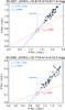 |
Fig. 2 Flux − flux diagram of quasi-simultaneous H vs. K measurements taken with a time separation of less than two hours (black dots with error bars). The data are linearly fit by the blue solid line, with an uncertainty range indicated by the blue dotted lines. The fit parameters are labeled in the upper left corner. The red long-dashed line and the red circle show the constraints for an additional non-varying CSD, derived from the color temperature Tvar of the varying star and the mean SEDs shown in Fig. 3. The blue dash-dotted lines mark the average H and K flux of the star, given by the difference between the black and red circles. |
Figure 2 shows the flux − flux diagram for the two sources ID 557 and ID 559. In this diagram, for each nearly simultaneous HK observation FH is plotted versus FK (black dots with error bars). The variability data clearly follow a linear relation. The blue solid line marks the slope β of the fitted linear relation FH = α + β·FK; this is the FVG. The blue dotted lines delineate the fit uncertainty of the gradient. The scatter of the data around the gradient is larger than expected from the error bars. An explanation could be that the H and K observations were obtained with a lag of about one hour, and so not sufficiently simultaneous given the strong variations from one day to the next.
The existence of a linear HK flux relationship shows that the variable component is intrinsically (i.e. before reddening) hot enough to be approximated by the Rayleigh-Jeans tail of a blackbody. The FVG slope gives to first order the HK color temperature, Tvar, of the variable component. The apparent Tvar values of 1352 K and 2089 K (Fig. 2) are obviously too low for a stellar source. However, they turn into physically meaningful stellar temperature ranges when proper dereddening is applied (see Sect. 5). Then Tvar lies well above the expected sublimation temperature of dust (Tdust < 2000 K), eliminating the possibility that the variations are dominated by temperature changes of the dust.
To facilitate the illustration of the FVG method, here we tentatively assume that the varying component is the star itself peppered with hot spots (T ~ 8000 K); variations of the CSD, the reflection nebula, or the envelope are neglected. In Sect. 6 we discuss alternatives to these assumptions; however, they do not affect the basic conclusions from the FVG technique.
A striking feature of both YSOs in Fig. 2 is that the FVG hits the x-axis at K ≈ 0.5 mJy and does not pass through the origin of the diagrams. We note that this is equivalent to the fact that the shorter wavelength (H) varies with larger amplitude than the longer wavelength (K)1. Because the flux variations follow a linear gradient over a large range, it is unlikely that the gradient will change to hit the origin if the star fades below its currently measured H band minimum. Instead, the flux zero point of the star might lie somewhere on the gradient between the lowest measured H flux and H = 0. This suggests the presence of an additional component that is cooler than the varying star.
For the further illustration of the FVG, we assume that this additional cool component is the CSD; the envelope is expected to be too cold to contribute at JHK. We note that for ID 559 the K band excess already implies the presence of such a CSD component; for ID 557 the HKL data suggest the presence of warm dust. The location of the CSD in Fig. 2 is marked with a red circle, and we justify the CSD color estimates in Sect. 4. Any CSD variations are either negligible or on an uncorrelated time scale different from that of the star, as indicated by the small scatter of the data points around the gradient.
The two selected sources, and almost all sources in RCW 38 with large variability amplitudes A show a linear relationship between FH and FK. About 50% of the 122 variable sources have A> 0.4. About 90% of them clearly show a linear gradient, which for ~80% of the sources does not go through the origin of the flux-flux diagram.
4. Decomposition of the mean JHKL SEDs
To constrain in Fig. 2 the zero point of the star on the FVG and the contribution of the inferred CSD, we make use of the mean SED in JHK and L (i.e. Spitzer/IRAC 3.6 μm). While the L band data were measured at a different epoch, one can expect that the CSD outshines any stellar contribution at L, hence that any variability at L is small compared to JHK.
Figure 3 shows the mean SEDs at JHKL. The HK color temperature Tvar of the star as determined from the FVG analysis is bluer than that of the total source. For simplicity we model the star’s JHKL SED as a blackbody with temperature Tvar. This allows us to constrain the maximum possible stellar flux, such that it matches the total SED at the J band; in this case we assume that the J band emission of the CSD is negligible.
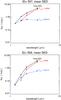 |
Fig. 3 Mean spectral energy distributions of ID 557 and 559. The total SED (black) is decomposed into a star (blue) and a circumstellar disk (red). The color temperature of the star is identified with Tvar as determined from the FVG analysis (Fig. 2). The star’s maximum possible mean flux is constrained by the lowest total SED, here the J band flux. The remaining SED (total minus star, depicted as red diamonds and connected by red solid lines) is fitted by a blackbody (red dotted line). The sum of the star and the CSD blackbody yields the “modeled” total SED (black dotted lines). |
To check whether the remaining SED (total SED minus maximum possible star) has a reasonable shape consistent with expectations for a CSD, we fit it by a blackbody leaving temperature and intensity as free parameters. As shown in Fig. 3, the fit deviates from the data by less than 20%. Furthermore, the sum of the star and the dust black bodies yields the modeled total SED (black dotted lines). Again, the fit at HKL is good; at J the modeled total SED lies slightly above the data, but this is expected from setting the star’s flux equal to the total J flux.
The resulting mean HK fluxes for the CSDs are plotted as red circles in Fig. 2 and the maximum possible average star fluxes are marked with the dashed-dotted blue lines (difference between mean star flux and mean CSD). The true contribution of the CSD and the star may be a bit larger/smaller, respectively, because in the above calculation we have assumed that the CSD does not emit at J and that the stellar SED follows a blackbody.
Of course, there may be alternatives to providing constraints on decomposing the SEDs and fitting a star and a CSD. The investigation of alternatives is postponed to the future.
5. Dereddening of star and disk
In Fig. 2 the derived HK color temperature of star and CSD are about Tstar ≈ 1300,2100 K and Tdust ≈ 800,1100 K. This is much lower than the range expected for an unreddened PMS star, with Tstar ≈ 3000 − 8000 K and hot dust (Tdust ≈ 1500 K) in the CSD. Thus, we check if reddening has shifted Tstar and Tdust from reasonable temperatures to the observed low values.
We assume that both star and CSD are reddened by the same amount of extinction. Dereddening the JHKL photometry by the AV values from Fig. 1 and the extinction curve from Rieke & Lebofsky (1985) we obtain dereddened flux-flux diagrams that look qualitatively similar to those in Fig. 2 but where the scaling differs in the sense that FH is more stretched than FK. For AV = 9 the dereddened values for ID 557 turn into Tstar ≈ 5800 K and Tdust ≈ 1350 K; an AV value of 10 mag yields Tstar ≈ 7700 K and Tdust ≈ 1400 K.
Notably, dereddening of ID 559 with AV = 10 (Fig. 1) yields Tstar ≈ 2300 and Tdust ≈ 1100 K, hence does not sufficiently raise the star and dust temperatures. However, increasing the visual extinction to AV = 17 mag yields Tstar ≈ 4900 K and Tdust ≈ 1350 K. In the JHK color−color diagram dereddening with AV = 17 shifts ID 559 below the CTTS line (Fig. 1). This apparent inconsistency could be explained by an unresolved reflection nebula diluting the actual reddening (e.g. Stark et al. 2006; Krügel 2009).
6. Discussion
Given the complexity of YSOs, the different components may contribute in a different manner to the variability observed across the optical, NIR and MIR wavelength range. Based on a simultaneous optical (R band) and MIR (IRAC 3.6−4.5 μm) variability study of NGC 2264, Cody et al. (2014) present an interesting discussion on different possible causes of the variability. For essentially all disk-bearing sources the variations at both IRAC filters are correlated. These variations are also correlated with the R band variations in 40% of the sources, indicating increased heating of the disk in response to variable accretion or hot spots on the surface of the star. For the remaining 60% of the Cody et al. sample with uncorrelated optical and MIR variability, we propose an alternative explanation.
It is thought that young stars are born as binaries or in multiple systems. If they are of different mass, the two binary components evolve differently, resulting in a blue star and an infrared star. They may show independent variations, the blue star dominating at optical and and the red star at MIR wavelengths. If such a binary is unresolved, an object with uncorrelated optical and MIR variability will be observed.
Swirling dust clouds (moving across the line of sight towards the star) produce varying extinction, resulting in a larger variability amplitude at the shorter wavelengths (e.g. Skrutskie et al. 1996; Carpenter et al. 2001; Indebetouw et al. 2006). Varying extinction may explain the variability behavior of UX Orionis stars believed to be seen at grazing angles of the disk (e.g. Herbst et al. 1994; Bertout 2000; Dullemond et al. 2003). If varying extinction is the dominant mechanism, then in a JHK color−color diagram or a color−magnitude diagram (CMD) the varying data points of each object should be aligned with the extinction vector. Such an alignment is only rarely found, e.g. in less than 10% of both the Carpenter et al. Orion data and our M 17 data (Scheyda 2010). For RCW 38, light curves are available only at H and K, but not at J. Our two YSOs (ID 557 and ID 559) show a clear elongation in the two CMDs H/(H − K) and K/(H − K), which however is not well aligned with the direction of the extinction vector2. We suggest that for both sources variable extinction may be present but that it plays a minor role.
As shown in Fig. 2, the CSD contributes to about 50% to the total H and K flux; this also holds for the dereddened data. Thus, after subtraction of the CSD, the two young stars have a huge variability amplitude (A ~ 20 for ID 557 and ID 559 reaches A ~ 100, equivalent to ~5 mag). This indicates that their luminosity is essentially powered by accretion bursts. Future studies may provide clues to whether such strong flux variations can be explained only by temperature and/or area changes of hot spots, or whether there are contributions from a variable hot gaseous disk in addition to the cooler CSD or whether the huge amplitudes are caused by other effects.
So far, with the aim of facilitating the illustration of the FVG method, we have neglected variations of the CSD, the reflection nebula, and the envelope3. Now we address these variations. If there is variable heating of the dust disk in response to variable accretion or hot spots on the surface of the star, and if the dust reacts quickly enough (e.g. simultaneously within the duration of the H and K observations), then the FVG measures a combination of the hot stellar and the cool dust flux variations. Then (after dereddening) Tvar is not the temperature of the varying stellar component ( ~ 8000 K), rather it is lowered by the contribution of the varying dust component (
 ~ 1500 K); hence Tvar underestimates . Accounting for the constant star and dust contributions and using Tvar instead of in the decomposition of the mean SED (Fig. 3) may result in an underestimation of the stellar flux at H and K, and hence an overestimation of the variability amplitude. A comprehensive treatment of the many combinations and aspects of NIR FVGs for YSOs, including the effects of reflection nebula and envelope, is planed for the future.
7. Summary and outlook
We have explored to what extent the flux variation gradient (FVG) technique can be transferred from active galactic nuclei to varying young stellar objects (YSOs). The results from HK monitoring data of the star forming region RCW 38 are as follows:
-
−
For almost all YSOs with large variability amplitudes the flux variations follow a linear relation FH = α + β·FK. Such a linear relation between fluxes from the two filters is consistent with the Rayleigh-Jeans approximation. In this case the FVG slope β gives the color temperature of the varying component.
-
−
Temperature considerations indicate that the star dominates the flux variations and that variations of the CSD/envelope or the reflection nebula play a minor role.
-
−
Two examples where the variability amplitudes are larger at shorter wavelengths and where variable extinction might play a minor role, are investigated in more detail. The negative FVG offsets (α< 0) imply the presence of an additional cool component such as a CSD. At least for some cases the FVG technique appears and better able to detect circumstellar disks than the K-excess in the JHK color color diagram. It appears worth using FVGs to reexamine the frequency of disks and the evolution of the disk dispersal in star forming clusters.
-
−
The low apparent HK color temperatures for the star and the disk, as inferred from FVGs, can be explained by substantial reddening. The extinction, required to deredden star and disk to realistic intrinsic temperatures, is at least as high as inferred from JHK color−color diagrams, consistent with extinction and scattering models.
-
−
FVGs provide basic input for the decomposition of SEDs. A more stringent SED decomposition requires further constraints that may be obtained from additional monitoring in a third filter and subsequent FVG analysis across several filter pairs.
-
−
After subtraction of the CSD, the two young stars investigated here display a huge variability amplitude (~3 − 5 mag). If the high amplitudes are not produced by other effects to be explored, the luminosity of these YSOs is essentially powered by accretion bursts.
To give an outlook on further applications, we have tentatively applied the FVG technique to two data sets:
-
−
Simultaneous JHK monitoring of the star forming region M 17 with the Infrared Service Facility (IRSF) at the 1.4 m telescope in Sutherland, South Africa (Scheyda 2010) yield for both filter combinations, JH and HK, that the flux variations follow a linear relation extremely well; Tvar agrees within the errors. We note that JK is redundant, being the product of JH and HK. The low scatter around the FVG is probably also a consequence of the perfect simultaneity of the observations. There are YSOs where the HK FVG with negative α implies a CSD; simultaneously the JH FVG has a positive α> 0 implying a reflection nebula or – more consistent with the unresolved appearance on optical BVRI images – an unresolved blue companion star. Since it is suspected that YSOs are born in multiple systems, such a companion is not unexpected, but needs to be verified. For instance, the young PMS binary XZ Tau consists of a rather evolved blue star and a less evolved infrared star (Haas et al. 1990).
The YSOVAR project lists Spitzer/IRAC 3.6 and 4.5 μm monitoring photometry of IC 1396 A and Orion (Morales-Calderón et al. 2009, 2011). Three hundred and eighty-seven Orion sources have amplitudes A> 0.2, and we find that their 3.6 and 4.5 μm flux variations follow a linear relation. For 154 of these sources (40%) we find Tvar> 1500 K, and for 64 sources (16%) Tvar> 2000 K, reaching 3500 K. Given that the sources are reddened, the variable component of these sources appears too hot to be dust. On the other hand, at 3.6 and 4.5 μm most of the emission is due to the inner disk and envelope, if present (e.g. Rebull et al. 2014). To bring both findings into a consistent picture, both stars and disk/envelope may vary simultaneously with similar strength so that the FVG measures an average Tvar, higher than for dust, but slightly lower than for the star.
The amplitudes A = (max − min) /avg are A(H) = 0.49, A(K) = 0.32 for ID 557 and A(H) = 0.84, A(K) = 0.44 for ID 559.
The resulting ratios AH/AK are 1.84 ± 0.09 and 2.19 ± 0.10 for ID 559 and ID 557, respectively, which is 3.1 σ and 6.2 σ from the standard extinction law (AH/AK = 1.56, with a ratio of total to selective extinction R ~ 3.1, Rieke & Lebofsky 1985). A much larger value R ~ 4 (e.g. Hoffmeister et al. 2008) would be required (locally at the sources) to align the H and K variability of ID 559 and ID 557 with the direction of the extinction vector. Such a large R value does not fit the overall consistency of the RCW 38 sources in the JHK color−color diagram with the standard extinction law (e.g. Fig. 3 in Dörr et al. 2013).
The assumption that the variations also occur in the CSD implies the existence of a CSD. Hence, in this case the FVG technique reveals the presence of a CSD.
Acknowledgments
This work is supported by the Nordrhein-Westfälische Akademie der Wissenschaften und der Künste in the framework of the academy program of the Federal Republic of Germany and the state Nordrhein-Westfalen, by Deutsche Forschungsgemeinschaft (DFG HA3555/12-1) and by Deutsches Zentrum für Luft-und Raumfahrt (DLR 50 OR 1106). This research has made use of NASA’s Astrophysics Data System. We thank the anonymous referee for constructive comments and careful review of the manuscript.
References
- Bertout, C. 2000, A&A, 363, 984 [NASA ADS] [Google Scholar]
- Carpenter, J. M., Hillenbrand, L. A., & Skrutskie, M. F. 2001, AJ, 121, 3160 [NASA ADS] [CrossRef] [Google Scholar]
- Choloniewski, J. 1981, Acta Astron., 31, 293 [NASA ADS] [Google Scholar]
- Cody, A. M., Stauffer, J., Baglin, A., et al. 2014, AJ, 147, 82 [NASA ADS] [CrossRef] [Google Scholar]
- Dörr, M., Chini, R., Haas, M., Lemke, R., & Nürnberger, D. 2013, A&A, 553, A48 [NASA ADS] [CrossRef] [EDP Sciences] [Google Scholar]
- Dullemond, C. P., van den Ancker, M. E., Acke, B., & van Boekel, R. 2003, ApJ, 594, L47 [NASA ADS] [CrossRef] [Google Scholar]
- Glass, I. S. 2004, MNRAS, 350, 1049 [NASA ADS] [CrossRef] [Google Scholar]
- Haas, M., Leinert, C., & Zinnecker, H. 1990, A&A, 230, L1 [NASA ADS] [Google Scholar]
- Haas, M., Chini, R., Ramolla, M., et al. 2011, A&A, 535, A73 [NASA ADS] [CrossRef] [EDP Sciences] [Google Scholar]
- Herbst, W., Herbst, D. K., Grossman, E. J., & Weinstein, D. 1994, AJ, 108, 1906 [NASA ADS] [CrossRef] [Google Scholar]
- Hodapp, K. W., Chini, R., Reipurth, B., et al. 2010, in SPIE Conf. Ser., 7735, 1 [Google Scholar]
- Hoffmeister, V. H., Chini, R., Scheyda, C. M., et al. 2008, ApJ, 686, 310 [NASA ADS] [CrossRef] [Google Scholar]
- Indebetouw, R., Whitney, B. A., Johnson, K. E., & Wood, K. 2006, ApJ, 636, 362 [NASA ADS] [CrossRef] [Google Scholar]
- Kenyon, S. J., Calvet, N., & Hartmann, L. 1993, ApJ, 414, 676 [NASA ADS] [CrossRef] [Google Scholar]
- Krügel, E. 2009, A&A, 493, 385 [NASA ADS] [CrossRef] [EDP Sciences] [Google Scholar]
- Meyer, M. R., Calvet, N., & Hillenbrand, L. A. 1997, AJ, 114, 288 [NASA ADS] [CrossRef] [Google Scholar]
- Morales-Calderón, M., Stauffer, J. R., Rebull, L., et al. 2009, ApJ, 702, 1507 [NASA ADS] [CrossRef] [Google Scholar]
- Morales-Calderón, M., Stauffer, J. R., Hillenbrand, L. A., et al. 2011, ApJ, 733, 50 [NASA ADS] [CrossRef] [Google Scholar]
- Pozo Nuñez, F., Ramolla, M., Westhues, C., et al. 2012, A&A, 545, A84 [NASA ADS] [CrossRef] [EDP Sciences] [Google Scholar]
- Pozo Nuñez, F., Westhues, C., Ramolla, M., et al. 2013, A&A, 552, A1 [NASA ADS] [CrossRef] [EDP Sciences] [Google Scholar]
- Pozo Nuñez, F., Haas, M., Chini, R., et al. 2014, A&A, 561, L8 [NASA ADS] [CrossRef] [EDP Sciences] [Google Scholar]
- Pozo Nuñez, F., Ramolla, M., Westhues, C., et al. 2015, A&A, 576, A73 [NASA ADS] [CrossRef] [EDP Sciences] [Google Scholar]
- Rebull, L. M., Cody, A. M., Covey, K. R., et al. 2014, AJ, 148, 92 [NASA ADS] [CrossRef] [Google Scholar]
- Rieke, G. H., & Lebofsky, M. J. 1985, ApJ, 288, 618 [NASA ADS] [CrossRef] [Google Scholar]
- Sakata, Y., Minezaki, T., Yoshii, Y., et al. 2010, ApJ, 711, 461 [NASA ADS] [CrossRef] [Google Scholar]
- Scheyda, C. M. 2010, Ph.D. Thesis, Ruhr-Universität Bochum [Google Scholar]
- Skrutskie, M. F., Meyer, M. R., Whalen, D., & Hamilton, C. 1996, AJ, 112, 2168 [NASA ADS] [CrossRef] [Google Scholar]
- Stark, D. P., Whitney, B. A., Stassun, K., & Wood, K. 2006, ApJ, 649, 900 [NASA ADS] [CrossRef] [Google Scholar]
- Winkler, H., Glass, I. S., van Wyk, F., et al. 1992, MNRAS, 257, 659 [NASA ADS] [Google Scholar]
- Winston, E., Wolk, S. J., Bourke, T. L., et al. 2011, ApJ, 743, 166 [NASA ADS] [CrossRef] [Google Scholar]
All Figures
|
Fig. 1 Color−color diagram of variable sources in RCW 38. Black dots with error bars denote averaged photometric single observations from Dörr et al (2013). The main sequence is shown in blue and the locus of unreddened classical T Tauri stars (CTTS) by the red long-dashed line. Two sources with ID 557 and 559 are highlighted in red; the small circles mark the individual H and K measurements placed at mean J − H owing to the lack of J variability data; the large circles give the mean H − K. The AV vectors are based on Rieke & Lebofsky (1985). |
| In the text | |
|
Fig. 2 Flux − flux diagram of quasi-simultaneous H vs. K measurements taken with a time separation of less than two hours (black dots with error bars). The data are linearly fit by the blue solid line, with an uncertainty range indicated by the blue dotted lines. The fit parameters are labeled in the upper left corner. The red long-dashed line and the red circle show the constraints for an additional non-varying CSD, derived from the color temperature Tvar of the varying star and the mean SEDs shown in Fig. 3. The blue dash-dotted lines mark the average H and K flux of the star, given by the difference between the black and red circles. |
| In the text | |
|
Fig. 3 Mean spectral energy distributions of ID 557 and 559. The total SED (black) is decomposed into a star (blue) and a circumstellar disk (red). The color temperature of the star is identified with Tvar as determined from the FVG analysis (Fig. 2). The star’s maximum possible mean flux is constrained by the lowest total SED, here the J band flux. The remaining SED (total minus star, depicted as red diamonds and connected by red solid lines) is fitted by a blackbody (red dotted line). The sum of the star and the CSD blackbody yields the “modeled” total SED (black dotted lines). |
| In the text | |
Current usage metrics show cumulative count of Article Views (full-text article views including HTML views, PDF and ePub downloads, according to the available data) and Abstracts Views on Vision4Press platform.
Data correspond to usage on the plateform after 2015. The current usage metrics is available 48-96 hours after online publication and is updated daily on week days.
Initial download of the metrics may take a while.