| Issue |
A&A
Volume 578, June 2015
|
|
|---|---|---|
| Article Number | A38 | |
| Number of page(s) | 7 | |
| Section | The Sun | |
| DOI | https://doi.org/10.1051/0004-6361/201425388 | |
| Published online | 01 June 2015 | |
Solar type II radio bursts associated with CME expansions as shown by EUV waves
IP&D – Universidade do Vale do Paraíba – UNIVAP,
Av. Shishima Hifumi, 2911 Urbanova,
São José dos Campos
SP,
Brazil
e-mail:
This email address is being protected from spambots. You need JavaScript enabled to view it.
Received: 21 November 2014
Accepted: 9 April 2015
Abstract
Aims. We investigate the physical conditions of the sources of two metric type II bursts associated with coronal mass ejection (CME) expansions with the aim of verifying the relationship between the shocks and the CMEs by comparing the heights of the radio sources and of the extreme-ultraviolet (EUV) waves associated with the CMEs.
Methods. The heights of the EUV waves associated with the events were determined in relation to the wave fronts. The heights of the shocks were estimated by applying two different density models to the frequencies of the type II emissions and compared with the heights of the EUV waves. For the event on 13 June 2010 that included band-splitting, the shock speed was estimated from the frequency drifts of the upper and lower frequency branches of the harmonic lane, taking into account the H/F frequency ratio fH/fF = 2. Exponential fits on the intensity maxima of the frequency branches were more consistent with the morphology of the spectrum of this event. For the event on 6 June 2012 that did not include band-splitting and showed a clear fundamental lane on the spectrum, the shock speed was directly estimated from the frequency drift of the fundamental emission, determined by linear fit on the intensity maxima of the lane. For each event, the most appropriate density model was adopted to estimate the physical parameters of the radio source.
Results. The event on 13 June 2010 had a shock speed of 590–810 km s-1, consistent with the average speed of the EUV wave fronts of 610 km s-1. The event on 6 June 2012 had a shock speed of 250–550 km s-1, also consistent with the average speed of the EUV wave fronts of 420 km s-1. For both events, the heights of the EUV wave revealed to be compatible with the heights of the radio source, assuming a radial propagation of the type-II-emitting shock segment.
Key words: Sun: radio radiation / Sun: corona / Sun: flares / Sun: coronal mass ejections (CMEs)
© ESO, 2015
1. Introduction
Radio emission stripes that slowly drift from high to low frequencies in the solar dynamic spectra are known as type II bursts and are generated from plasma oscillations that are attributed to a fast-mode magnetohydrodynamic (MHD) shock waves (Nelson & Melrose 1985). The shock propagates outwards through the corona at speeds of 200 to 2000 km s-1, as shown by the drifts of the emissions towards lower frequencies owing to the decreasing ambient density. Radial speeds can be deduced from the drift rates (~0.1–1.5 MHz s-1) of the emissions by using coronal density models.
Type II bursts were suggested to be signatures of shock waves by Uchida (1960) and Wild (1962), and the first evidence of this association came from the interpretation of the Moreton waves (Moreton 1960), which are large-scale wave-like disturbances in the chromosphere observed in Hα. The Moreton waves propagate out of the flare site at speeds in the order of those of the shock waves that, at greater heights, cause type II bursts.
The emissions are observed at multiples of the electron plasma frequency, given by ![Mathematical equation: \hbox{$f_{\rm{p}}=8.98 \times 10^{-3} \sqrt{n_{\rm{e}}} \ \ [\mathrm{MHz}] $}](/articles/aa/full_html/2015/06/aa25388-14/aa25388-14-eq5.png) , chiefly at the fundamental and second harmonic emissions. Sometimes the third harmonic emission can be observed in the dynamic spectra of type II bursts (see, e.g., Zlotnik et al. 1998).
, chiefly at the fundamental and second harmonic emissions. Sometimes the third harmonic emission can be observed in the dynamic spectra of type II bursts (see, e.g., Zlotnik et al. 1998).
In the meter wavelength range, type II bursts typically show a starting frequency for the fundamental emission around 100 MHz. Nevertheless, it is common to observe events with considerably higher starting frequencies (see, e.g., Vršnak et al. 2002; Reiner et al. 2003; Vršnak & Cliver 2008). The events last for several minutes (~1–15 min), and sometimes the emission stripes are split into two parallel lanes (band-splitting effect); the mechanism that causes this is not fully understood as yet (see, e.g., Tidman et al. 1966; Krüger 1979; Treumann & Labelle 1992). One feasible and potential interpretation of this effect was proposed by Smerd et al. (1974) in terms of the emission from the upstream and downstream shock regions, which associates this effect with an abrupt density variation at the shock front (see, e.g., Vršnak et al. 2001, 2002; Cho et al. 2007; Zimovets et al. 2012).
Although the association between type II bursts and coronal shock waves is well established, the physical relationship among metric type II bursts, flares, and coronal mass ejections (CMEs) is only poorly understood. A causal relationship between metric type II bursts and CMEs is a controversial question (see, e.g., Cliver et al. 2004; Vršnak & Cliver 2008; Prakash et al. 2010), whereas for type II bursts at dekameter and longer wavelengths there is a consensus that they are driven by CMEs (see, e.g., Cane et al. 1987; Gopalswamy et al. 2000). According to Vršnak & Cliver (2008), the source of the coronal wave seems clear in some events with starting frequencies well below 100 MHz, where the CME is accompanied only by a very weak or gradual flare-like energy release. On the other hand, according to these authors, for Moreton-wave-associated type II bursts, that have considerably higher frequencies (>300 MHz for the harmonic emission), both the CME and the flare are observed. In these cases, the CME and the flare are often tightly related and, particularly during the impulsive phase, motions of the flare plasma take place together with the CME motions, and both phenomena are potential sources of the shocks (for a discussion see, e.g., Vršnak & Cliver 2008; Magdalenić et al. 2012).
The study of the relationship between type II bursts and CMEs can be improved by observations of propagating brightness fronts in the extreme ultraviolet (EUV), so-called EUV waves (see, e.g., Moses et al. 1997; Thompson et al. 1998). The onsets of expanding dimmings that occasionally accompany the EUV waves indicate the source regions of the CME and are related to its fast acceleration phase (see, e.g., Cliver et al. 2004). The wave nature of the EUV waves, however, is still under debate. In wave models, they are interpreted as a fast-mode wave, most likely triggered by a CME, and represent the coronal counterpart of the Moreton waves (see, e.g., Vršnak & Cliver 2008; Patsourakos & Vourlidas 2012). In the non-wave models, they are explained by other processes related to the large-scale magnetic field reconfiguration and can be interpreted as a disk projection of the expanding envelope of the CME (see, e.g., Delannée & Aulanier 1999; Chen et al. 2005; Attrill et al. 2007), being usually much slower and more diffuse (see, e.g., Klassen et al. 2000; Warmuth et al. 2004a,b). According to Klassen et al. (2000), 90% of the metric type II bursts are associated with EUV waves, but there is no correlation between their speeds.
Given that metric type II bursts are somewhat rarer than the number of flares and CMEs, case studies are helpful in investigating the dynamic behavior of the shocks associated with these phenomena (for a detailed analysis of CME-type II relationship see, e.g., Magdalenić et al. 2010). In studying the physical conditions of the sources of two metric type II bursts associated with CME expansions as shown by EUV waves, we aim to verify the relationship between the radio sources and the CMEs mainly in terms of the heights and speeds of the EUV wave fronts and the type II sources.
2. Observations and analysis
The type II events investigated in this article were observed by two spectrometers from extended-Compound Astronomical Low-cost Low-frequency Instrument for Spectroscopy and Transportable Observatories (e-CALLISTO)1. The dynamic spectra of the type II bursts were digitally recorded with time and frequency resolutions of 1.25 ms and 62.5 kHz (see, e.g., Benz et al. 2009).
2.1. Event on 13 June 2010
The event on 13 June 2010 (hereafter event 1) was observed at ~05:37:10 UT by CALLISTO-OOTY (Ooty, India) in the operational frequency range of 45–442 MHz and was included in the Burst Catalog, built by C. Monstein2. This event was also observed by the radio spectrograph of Learmonth Observatory (Kozarev et al. 2011), the radio spectrograph of San Vito Observatory (Ma et al. 2011), the Hiraiso Radio Spectrograph (Gopalswamy et al. 2012), and the radio spectrograph ARTEMIS IV (Kouloumvakos et al. 2014).
Figure 1 shows that both the fundamental and harmonic emissions are present in the dynamic spectrum of event 1, with the fundamental lane being partially reabsorbed. The bright branches of the harmonic emission showed a clear-cut band-splitting effect, with an onset at ~325 MHz. Although partially reabsorbed, the band-splitting effect for the fundamental emission was also observed in the spectrum.
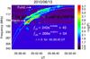 |
Fig. 1 Dynamic spectrum of the type II burst (left panel) observed by CALLISTO-OOTY on June 13, 2010 at ~05:37:10 UT, with exponential fits for the upper (UB) and the lower (LB) frequency branches of the harmonic lane. |
Event 1 was accompanied by a slow CME (~320 km s-1), observed by the Large Angle and Spectrometric Coronagraph (LASCO-C2/C3) onboard the Solar and Heliospheric Observatory (SoHO), with onset at ~05:14 UT, according to linear backward-extrapolation of the heights, provided by the LASCO CME Catalog. In addition, an M1.0 SXR flare, observed by the Geostationary Operational Environmental Satellites (GOES), with onset at ~05:30 UT and peak at ~05:39 UT, was also associated with event 1. Both the CME and the flare associated with event 1 originated from the active region NOAA 11079, close to the solar limb (S25W84).
The EUV wave associated with event 1, observed by the Extreme Ultraviolet Imaging Telescope (EIT) onboard SoHO and by the Atmospheric Imaging Assembly (AIA) onboard the Solar Dynamics Observatory (SDO) are shown in Figs. 2 and 3.
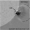 |
Fig. 2 Base-difference image of SoHO/EIT 195 Å showing the EUV wave associated with the type II emission. |
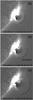 |
Fig. 3 Base-difference images of SDO/AIA 211 Å showing the CME expansion and the EUV wave associated with event 1 for: a) 05:38–05:35 UT; b) 05:39–05:35 UT; and c) 05:40–05:35 UT. |
Exponential fits on the intensity maxima of the upper and lower frequency branches of the harmonic lane of event 1 used to estimate the frequency drift rate [df/ dt] of the emission were more consistent with the morphology of the spectrum of the event and provided − (1.11–0.37) MHz s-1. This result implies a drift of − (0.55–0.18) MHz s-1 for the fundamental emission, taking into account the H/F frequency ratio fH/fF = 2.
The instantaneous band split, given by BDi = fUB − fLB, taken at each time step of 0.25 s, was in the range of 13–29 MHz for the harmonic emission of event 1.
2.2. Event on 6 June 2012
The event on 6 June 2012 (hereafter event 2) was observed at ~20:03:25 UT by CALLISTO-BIR (Birr, Ireland) in the operational frequency range of 10–196 MHz. Figure 4 shows the dynamic spectrum of event 2 with both the fundamental and the harmonic emissions, despite the radio frequency interference at ~90–120 MHz. A type II precursor (see, e.g., Klassen et al. 1999; Vršnak & Lulić 2000) at ~20:01:40 UT is also present in the spectrum of event 2.
Event 2 was associated with a CME with a linear speed of ~494 km s-1, observed by LASCO-C2/C3 onboard SoHO, with onset at ~19:37 UT, according to linear backward-extrapolation of the heights, provided by the LASCO CME Catalog. An M2.1 SXR flare, observed by GOES, with onset at ~19:54 UT and peak at ~20:06 UT, was also associated with event 2. Both the CME and the flare associated with event 2 originated from the active region NOAA 11494 on the solar disk (S17W08).
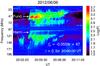 |
Fig. 4 Dynamic spectrum of the type II burst observed by CALLISTO-BIR on June 6, 2012 at ~20:03:25 UT, with linear fit for the fundamental lane. |
The expansion of the CME associated with event 2 was clear from the EUV images provided by the Extreme Ultraviolet Imager (EUVI) onboard the Solar Terrestrial Relations Observatory (STEREO) presented in Fig. 5.
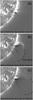 |
Fig. 5 Base-difference images of STEREO/SECCHI/EUVI-B 195 Å for: a) 20:00–19:50 UT (initial expansion of the CME, ~3 min before the onset of the type II emission); b) 20:05–19:50 UT (fast expansion of the CME during the intensification of the type II emission); and c) 20:10–19:50 UT (disruption of the CME flux rope at the end of the type II emission). |
Event 2 showed an intense fundamental emission with a herringbone-like feature (see, e.g., Mann & Classen 1995) and with a linear-like frequency drift. A linear fit on the intensity maxima of the fundamental lane provided a frequency drift rate of −0.056 MHz s-1. Event 2 presented an instantaneous bandwidth [Δfi] of 5–26 MHz for the fundamental lane, adopting the half-flux bandwidths of the maxima of the emission. Since there was no band-splitting for event 2, a different approach was used, and the instantaneous bandwidth was adopted in place of the instantaneous band split, similar to that used by Mann et al. (1995).
3. Physical parameters: models and equations
From the observational parameters of the type II bursts, it is possible, with some assumptions, to estimate the physical parameters of the radio sources. In this section, we present the models and equations adopted in this article.
In most cases, the use of the 1–2×Newkirk (1961) density model to estimate the radio source speed is compatible with a radial shock motion (see, e.g., Vršnak et al. 2001), whereas the use of the 3–4×Newkirk (1961) model is suitable for an oblique propagation of the type-II-emitting shock segment (see, e.g., Klassen et al. 1999; Classen & Aurass 2002; Cunha-Silva et al. 2014), avoiding the underestimation of the shock speed. The Newkirk (1961) density model is given by 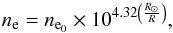 (1)where ne0 = 4.2 × 104 cm-3, R is the heliocentric distance and R⊙ is the solar radius.
Cairns et al. (2009) extracted ne(R) directly from coronal type III radio bursts for 40 ≤ f ≤ 180 MHz and found ne ∝ (R − R⊙)-2 for R< 2 R⊙ (note that for R ≫ R⊙ this falloff becomes ne ∝ R-2, which is a standard solar wind property that holds for R ≥ 10 R⊙). Thus, we adopted 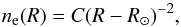 (2)where C is a constant determined from the time-varying radiation frequency and the radial speed of the source.
We compared these two different density-height models applied to the type II events with the heights of the associated EUV waves with the aim of determining which model is more appropriate to be adopted in estimating the physical parameters of the radio sources.
A practical expression for the radial speed of the shock [dR/ dt], for n×Newkirk (1961) density model, is (Cunha-Silva et al. 2014)  (3)The density jump at the shock front [Xn] is determined from the relative instantaneous band split [BDi/fLB] (Vršnak et al. 2002):
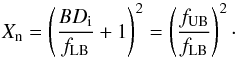 (4)For a shock perpendicular to the magnetic field and β → 0, the Alfvén Mach number [MA] is (Vršnak et al. 2002)
 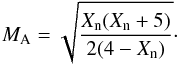 (5)The Alfvén speed [vA], in turn, can be obtained directly from the shock speed [vs] and MA:
  (6)Finally, the magnetic-field strength [B] in regions of shock surrounding a CME can be estimated using (Kim et al. 2012)
 ![Mathematical equation: \begin{equation} B=5.0\times10^{-7}v_{\rm{A}}\sqrt{n_{\rm{e}}} \ \ [\mathrm{G}]. \label{eq7} \end{equation}](/articles/aa/full_html/2015/06/aa25388-14/aa25388-14-eq40.png) (7)
(7)
4. Results and discussion
We compared the heights of the EUV wave fronts with the heights of the radio sources and then estimated the physical parameters of the radio sources by applying the more appropriate coronal density model, taking into account that under the assumed band-split interpretation for event 1, the application of coronal density models to the lower-frequency branch is more appropriate to estimate the shock kinematics, since it represents the emission from undisturbed corona.
4.1. Event 1
Figure 6 shows the type II heights, obtained with the density models of 1–2×Newkirk (1961) and of Cairns et al. (2009), and the heights of the EUV wave fronts associated with event 1. We adopted 10% of the measures for the error bars of the EUV wave fronts, considering the uncertainties of 7–12% in the measurements.
Figure 6 shows that the heights of the EUV wave fronts associated with event 1 are consistent with the heights of the type II emission obtained with the density models of 1×Newkirk (1961) and of Cairns et al. (2009) for the first five minutes of the event, supporting a quasi-radial propagation of the type-II-emitting shock segment.
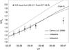 |
Fig. 6 Comparison of the type II heights, obtained with the density models of 1–2×Newkirk (dashed lines) and Cairns et al. (2009; solid line), applied to the frequencies provided by the exponential fit on the intensity maxima of the lower-frequency branch, with the heights of the EUV wave fronts (five data points from SDO/AIA 211 Å, limited by the field of view (FOV) of the instrument, and one data point from SoHO/EIT 195 Å, at the end of the type II emission), for event 1. The models of 1×Newkirk and of Cairns et al. (2009) provided similar results for event 1. |
Given that the models of 1×Newkirk (1961) and of Cairns et al. (2009) provided results consistent with the heights of the EUV wave fronts for event 1, we adopted the former to estimate the physical parameters of the radio source for this event. In Fig. 7, the physical parameters of the radio source for event 1 are presented as a function of the heliocentric distance. The error bars of the estimates were defined as the instrumental errors of the measures, considering a quadratic error equal to zero.
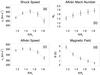 |
Fig. 7 Physical parameters of the radio source for event 1: a) shock speed, calculated from the frequency drift [df/ dt] and the plasma frequency [fp]; b) Alfvén Mach number, calculated from the density jump at the shock front [Xn]; c) Alfvén speed, calculated from the shock speed [vs] and the Alfvén Mach number [MA]; and d) magnetic field strength, calculated from the electron number density [ne] and the Alfvén speed [vA]. The values were determined with respect to the central frequencies of the lower-frequency branch of the radio emission. |
Figure 7a shows that a shock speed of 590–810 km s-1 as found for event 1 is consistent with the initial and average speeds of the EUV wave fronts of 720 and 610 km s-1. Our results show an accelerating shock with a speed of 665–810 km s-1 during the first five minutes of the type II emission, followed by a shock deceleration, with speeds of 810 to 590 km s-1 for the following five minutes of the event, which is consistent with the strong acceleration (up to speeds of ~400 km s-1) followed by the deceleration of the EUV bubble associated with the CME, found by Patsourakos et al. (2010). A similar behavior was reported by Gopalswamy et al. (2012), who found an accelerating shock with speeds of ~590–720 km s-1 for the first three minutes of the type II emission, followed by a shock deceleration with speeds of ~720 to 640 km s-1 for the next two minutes. The adoption of the central frequencies of the lower-frequency branch to estimate the heights of the radio source has accounted for our higher values. However, our results are different from those obtained by Vasanth et al. (2014), who found a sharp decrease in the shock speed, from 820 km s-1 to 580 km s-1, for 05:39–05:41 UT (three and five minutes after the onset of the type II emission). Our estimates of the frequency drift rate using exponential fits on the intensity maxima of the radio emission may be responsible for these differences.
A slightly increasing Alfvén speed of 470–500 km s-1 for the first three minutes of event 1, followed by a decrease from 500 to 340 km s-1, shown in Fig. 7c, was the result of a direct determination of this parameter from the shock speed and the Alfvén Mach number, and is marginally compatible with the typical decrease of this parameter in regions of shock formation (R< 2 R⊙) (see, e.g., Vršnak et al. 2002). This finding, however, is somewhat different from that reported by Gopalswamy et al. (2012), who found a sharp increase in the Alfvén speed of ~140–460 km s-1 for the first three minutes of the type II emission, followed by a decrease from ~460 to 410 km s-1. The values found by us and by Gopalswamy et al. (2012) are below those reported by Vršnak et al. (2002), who found 600–1000 km s-1 for the heliocentric distances of ~1.2–1.8, applying a fifth degree polynomial fit on measurements based on observational data.
A magnetic field strength of 0.5–3.7 G, for the heliocentric distances of ~1.2–1.8, found for event 1, is consistent with the values of about 1.2–5.0 G reported by Vršnak et al. (2002) for these heliocentric distances, obtained by a power-law fit on measurements based on observational data, assuming the coronal density model of 2×Newkirk (1961). Considering the error bars of our estimates, shown in Fig. 7d, a magnetic field strength of 2.3 G for a shock speed of ~760 km s-1, obtained for three minutes after the onset of the type II emission, is consistent with the magnetic field strength of 1.7–1.9 G found by Kouloumvakos et al. (2014) for a shock speed of ~700 km s-1. Our higher values for the initial heights of the type II emission are due to our higher values for the Alfvén speed, even with our higher Alfvén Mach number of 1.4–1.7, against 1.3–1.5, found by Kouloumvakos et al. (2014). Our values for the Alfvén Mach number are consistent with the measurements of about 1.1–1.9 reported by Vršnak et al. (2002) for the heliocentric distances of ~1.3–2.5.
4.2. Event 2
Taking the analysis of event 1 as a touchstone for the analysis of event 2, we compared the heights of the EUV wave fronts with the heights of the radio source and determined the physical parameters of the radio source with the more appropriate model, adopting similar criteria and the same equations. Figure 8 shows the type II heights, obtained with the density models of 1–2×Newkirk (1961) and of Cairns et al. (2009) and the heights of the EUV wave fronts associated with event 2.
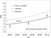 |
Fig. 8 Comparison of the type II heights obtained with the density models of 1–2×Newkirk (dashed lines) and of Cairns et al. (2009; solid line), applied to the frequencies provided by the linear fit on the intensity maxima of the fundamental emission, with the heights of the EUV wave fronts (three data points from STEREO/EUVI-B 195 Å) for event 2. Similarly as for event 1, the models of 1×Newkirk and of Cairns et al. (2009) are equivalent for event 2. |
As found for event 1, the heights of the EUV wave fronts associated with event 2 are consistent with the heights of the type II emission obtained with the density models of 1×Newkirk (1961) and of Cairns et al. (2009), as is clear from Fig. 8, supporting a quasi-radial propagation of the type-II-emitting shock segment. In this case, however, we found a radio source moving away from the Sun more slowly than the EUV wave fronts.
The morphology of the spectrum of event 2, with a linear-like frequency drift, accounts for the greater similarity between the results for the heights of the radio source provided by the density models of 1×Newkirk (1961) and of Cairns et al. (2009). Again, we adopted the former to estimate the physical parameters of the radio source of event 2. In Fig. 9, the physical parameters of the radio source for event 2 are presented as a function of the heliocentric distance.
In Fig. 9a, an accelerating shock with speeds of 250–550 km s-1 indicates radio emission from the early stages of a shock driven by CME expansion during its fast acceleration phase. This interpretation is consistent with the linear speed of the associated CME of 490 km s-1, which is higher than the average speed of the associated EUV wave fronts of 420 km s-1.
The Alfvén speed determined directly from the shock speed and the Alfvén Mach number, according to Eq. (6), showed a somewhat atypical behavior for event 2 that is due to a combination of an increasing shock speed with an increasing Alfvén Mach number of 1.1–2.1. Different from what was obtained for event 1, we found a slightly decreasing Alfvén speed of 230 to 220 km s-1, followed by an increase of 220–280 km s-1, shown in Fig. 9c. Our values for the Alfvén Mach number are consistent with the measurements of about 1.1–1.9 reported by Vršnak et al. (2002) for heliocentric distances of ~1.3–2.5.
Another interesting feature of Fig. 9d, is a comparatively slow decrease of the magnetic field strength, which becomes almost constant between R = 1.45 and 1.55. This somewhat atypical behavior could be attributed to the fact that the magnetic field strength estimate depends not only on the coronal density, but also on the estimate of the Alfvén speed based on Eq. (7), which accounts for this somewhat atypical behavior.
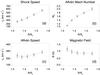 |
Fig. 9 Physical parameters of the radio source for event 2: a) shock speed, calculated from the frequency drift [df/ dt] and the plasma frequency [fp]; b) Alfvén Mach number, calculated from the density jump at the shock front [Xn]; c) Alfvén speed, calculated from the shock speed [vs] and the Alfvén Mach number [MA]; and d) magnetic field strength, calculated from the electron number density [ne] and the Alfvén speed [vA]. The values were determined with respect to the lower frequencies of the fundamental lane of the radio emission. |
5. Conclusions
We investigated two solar type II radio bursts associated with EUV waves, one of which included a split-band event, with the fundamental emission partially reabsorbed, that took place close to the limb, and one event without band-splitting, with both the fundamental and harmonic emissions intense on the spectrum, that took place on the disk. Both events agreed with the observational pattern reported by Biesecker et al. (2002) that type II events on the disk are often observed in the fundamental and harmonic emissions, whereas only the harmonic emission is usually observed for those at the limb.
For both events, the heights of the EUV wave fronts are compatible with the heights of the radio source obtained with the density models of 1×Newkirk (1961) and of Cairns et al. (2009), supporting a quasi-radial propagation of the type-II-emitting shock segment for the events.
The finding of an accelerating shock during the first five minutes of event 1, followed by a shock deceleration for the next five minutes of the event, is consistent with the strong acceleration followed by deceleration of the EUV bubble associated with the event found by Patsourakos et al. (2010) and is also consistent with a similar shock speed behavior reported by Gopalswamy et al. (2012) for the first five minutes of the event.
The finding of an accelerating shock throughout event 2 proved to be consistent with the kinematics of the EUV wave fronts, which we found to be moving faster than the radio source.
Our results support a close association between the radio source and the CME expansion for both events, as shown by the close relation between the type-II-emitting shock segment and the EUV wave, which clearly was produced by the CME.
The e-CALLISTO data are available at http://soleil.i4ds.ch/solarradio/data/2002-20yy_ Callisto/
Acknowledgments
The authors acknowledge financial support from the São Paulo Research Foundation (FAPESP), grant number 2012/08445-9. C.L.S. acknowledges financial support from the São Paulo Research Foundation (FAPESP), grant number 2014/10489-0. R.D.C.S. acknowledges a scholarship from the São Paulo Research Foundation (FAPESP), grant number 2012/00009-5, and financial support from UNIVAP-FVE. FCRF thanks CNPq for the scholarship granted under process 308755/2012-0. The authors are grateful to the e-CALLISTO science teams for the solar data. The EUV images were courtesy of ESA/NASA/ SoHO/EIT, NASA/STEREO/EUVI, and NASA/SDO/AIA consortia. The authors are grateful to the anonymous referee for the significant and constructive remarks that helped to improve the quality and presentation of this article.
References
- Attrill, G. D. R., Harra, L. K., van Driel-Gesztelyi, L., & Démoulin, P. 2007, ApJ, 656, L101 [NASA ADS] [CrossRef] [Google Scholar]
- Benz, A. O., Monstein, C., Meyer, H., et al. 2009, Earth Moon Planets, 104, 277 [NASA ADS] [CrossRef] [Google Scholar]
- Biesecker, D. A., Myers, D. C., Thompson, B. J., Hammer, D. M., & Vourlidas, A. 2002, ApJ, 569, 1009 [NASA ADS] [CrossRef] [Google Scholar]
- Cairns, I. H., Lobzin, V. V., Warmuth, A., et al. 2009, ApJ, 706, L265 [NASA ADS] [CrossRef] [Google Scholar]
- Cane, H. V., Sheeley, N. R. J., & Howard, R. A. 1987, J. Geophys. Res., 92, 9869 [NASA ADS] [CrossRef] [Google Scholar]
- Chen, P. F., Fang, C., & Shibata, K. 2005, ApJ, 622, 1202 [Google Scholar]
- Cho, K.-S., Lee, J., Gary, D. E., Moon, Y.-J., & Park, Y. D. 2007, ApJ, 665, 799 [NASA ADS] [CrossRef] [Google Scholar]
- Classen, H. T., & Aurass, H. 2002, A&A, 384, 1098 [NASA ADS] [CrossRef] [EDP Sciences] [Google Scholar]
- Cliver, E. W., Nitta, N. V., Thompson, B. J., & Zhang, J. 2004, Sol. Phys., 225, 105 [NASA ADS] [CrossRef] [Google Scholar]
- Cunha-Silva, R. D., Fernandes, F. C. R., & Selhorst, C. L. 2014, Sol. Phys., 289, 4607 [NASA ADS] [CrossRef] [Google Scholar]
- Delannée, C., & Aulanier, G. 1999, Sol. Phys., 190, 107 [NASA ADS] [CrossRef] [Google Scholar]
- Gopalswamy, N., Kaiser, M. L., Thompson, B. J., et al. 2000, Geophys. Res. Lett., 27, 1427 [NASA ADS] [CrossRef] [Google Scholar]
- Gopalswamy, N., Nitta, N., Akiyama, S., Mäkelä, P., & Yashiro, S. 2012, ApJ, 744, 72 [NASA ADS] [CrossRef] [Google Scholar]
- Kim, R.-S., Gopalswamy, N., Moon, Y.-J., Cho, K.-S., & Yashiro, S. 2012, ApJ, 746, 118 [NASA ADS] [CrossRef] [Google Scholar]
- Klassen, A., Aurass, H., Klein, K.-L., Hofmann, A., & Mann, G. 1999, A&A, 343, 287 [NASA ADS] [Google Scholar]
- Klassen, A., Aurass, H., Mann, G., & Thompson, B. J. 2000, A&AS, 141, 357 [NASA ADS] [CrossRef] [EDP Sciences] [Google Scholar]
- Kouloumvakos, A., Patsourakos, S., Hillaris, A., et al. 2014, Sol. Phys., 289, 2123 [NASA ADS] [CrossRef] [Google Scholar]
- Kozarev, K. A., Korreck, K. E., Lobzin, V. V., Weber, M. A., & Schwadron, N. A. 2011, ApJ, 733, L25 [NASA ADS] [CrossRef] [Google Scholar]
- Krüger, A. 1979, Introduction to Solar Radio Astronomy and Radio Physics (Dordrecht: D. Reidel Publishing Co.) [Google Scholar]
- Ma, S., Raymond, J. C., Golub, L., et al. 2011, ApJ, 738, 160 [CrossRef] [Google Scholar]
- Magdalenić, J., Marqué, C., Zhukov, A. N., Vrsnak, B., & Zic, T. 2010, ApJ, 718, 266 [NASA ADS] [CrossRef] [Google Scholar]
- Magdalenić, J., Marqué, C., Zhukov, A. N., Vršnak, B., & Veronig, A. 2012, ApJ, 746, 152 [NASA ADS] [CrossRef] [Google Scholar]
- Mann, G., & Classen, H. T. 1995, A&A, 304, 576 [NASA ADS] [Google Scholar]
- Mann, G., Classen, T., & Aurass, H. 1995, A&A, 295, 775 [NASA ADS] [Google Scholar]
- Moreton, G. E. 1960, AJ, 65, 494 [Google Scholar]
- Moses, D., Clette, F., Delaboudinière, J.-P., et al. 1997, Sol. Phys., 175, 571 [NASA ADS] [CrossRef] [Google Scholar]
- Nelson, G. J., & Melrose, D. B. 1985, in Solar Radiophysics, eds. D. J. McLean, & N. R. Labrum (Cambridge: Cambridge Univ. Press), 333 [Google Scholar]
- Newkirk, G. J. 1961, ApJ, 133, 983 [NASA ADS] [CrossRef] [Google Scholar]
- Patsourakos, S., & Vourlidas, A. 2012, Sol. Phys., 281, 187 [NASA ADS] [Google Scholar]
- Patsourakos, S., Vourlidas, A., & Stenborg, G. 2010, ApJ, 724, L188 [Google Scholar]
- Prakash, O., Umapathy, S., Shanmugaraju, A., Pappa Kalaivani, P., & Vršnak, B. 2010, Sol. Phys., 266, 135 [NASA ADS] [CrossRef] [Google Scholar]
- Reiner, M. J., Vourlidas, A., Cyr, O. C. S., et al. 2003, ApJ, 590, 533 [NASA ADS] [CrossRef] [Google Scholar]
- Smerd, S. F., Sheridan, K. V., & Stewart, R. T. 1974, IAU Symp., 57, 389 [Google Scholar]
- Thompson, B. J., Plunkett, S. P., Gurman, J. B., et al. 1998, Geophys. Res. Lett., 25, 2465 [Google Scholar]
- Tidman, D. A., Birmingham, T. J., & Stainer, H. M. 1966, ApJ, 146, 207 [NASA ADS] [CrossRef] [Google Scholar]
- Treumann, R. A., & Labelle, J. 1992, ApJ, 399, 167 [Google Scholar]
- Uchida, Y. 1960, PASJ, 12, 376 [NASA ADS] [Google Scholar]
- Vasanth, V., Umapathy, S., Vršnak, B., Žic, T., & Prakash, O. 2014, Sol. Phys., 289, 251 [NASA ADS] [CrossRef] [Google Scholar]
- Vršnak, B., & Cliver, E. W. 2008, Sol. Phys., 253, 215 [NASA ADS] [CrossRef] [Google Scholar]
- Vršnak, B., & Lulić, S. 2000, Sol. Phys., 196, 157 [Google Scholar]
- Vršnak, B., Aurass, H., Magdalenić, J., & Gopalswamy, N. 2001, A&A, 377, 321 [Google Scholar]
- Vršnak, B., Magdalenić, J., Aurass, H., & Mann, G. 2002, A&A, 396, 673 [NASA ADS] [CrossRef] [EDP Sciences] [Google Scholar]
- Warmuth, A., Vršnak, B., Magdalenić, J., Hanslmeier, A., & Otruba, W. 2004a, A&A, 418, 1101 [NASA ADS] [CrossRef] [EDP Sciences] [Google Scholar]
- Warmuth, A., Vršnak, B., Magdalenić, J., Hanslmeier, A., & Otruba, W. 2004b, A&A, 418, 1117 [NASA ADS] [CrossRef] [EDP Sciences] [Google Scholar]
- Wild, J. P. 1962, J. Phys. Soc. Japan, 17, 249 [Google Scholar]
- Zimovets, I., Vilmer, N., Chian, A. C. L., Sharykin, I., & Struminsky, A. 2012, A&A, 547, A6 [NASA ADS] [CrossRef] [EDP Sciences] [Google Scholar]
- Zlotnik, E. Y., Klassen, A., Klein, K. L., Aurass, H., & Mann, G. 1998, A&A, 331, 1087 [NASA ADS] [Google Scholar]
All Figures
|
Fig. 1 Dynamic spectrum of the type II burst (left panel) observed by CALLISTO-OOTY on June 13, 2010 at ~05:37:10 UT, with exponential fits for the upper (UB) and the lower (LB) frequency branches of the harmonic lane. |
| In the text | |
|
Fig. 2 Base-difference image of SoHO/EIT 195 Å showing the EUV wave associated with the type II emission. |
| In the text | |
|
Fig. 3 Base-difference images of SDO/AIA 211 Å showing the CME expansion and the EUV wave associated with event 1 for: a) 05:38–05:35 UT; b) 05:39–05:35 UT; and c) 05:40–05:35 UT. |
| In the text | |
|
Fig. 4 Dynamic spectrum of the type II burst observed by CALLISTO-BIR on June 6, 2012 at ~20:03:25 UT, with linear fit for the fundamental lane. |
| In the text | |
|
Fig. 5 Base-difference images of STEREO/SECCHI/EUVI-B 195 Å for: a) 20:00–19:50 UT (initial expansion of the CME, ~3 min before the onset of the type II emission); b) 20:05–19:50 UT (fast expansion of the CME during the intensification of the type II emission); and c) 20:10–19:50 UT (disruption of the CME flux rope at the end of the type II emission). |
| In the text | |
|
Fig. 6 Comparison of the type II heights, obtained with the density models of 1–2×Newkirk (dashed lines) and Cairns et al. (2009; solid line), applied to the frequencies provided by the exponential fit on the intensity maxima of the lower-frequency branch, with the heights of the EUV wave fronts (five data points from SDO/AIA 211 Å, limited by the field of view (FOV) of the instrument, and one data point from SoHO/EIT 195 Å, at the end of the type II emission), for event 1. The models of 1×Newkirk and of Cairns et al. (2009) provided similar results for event 1. |
| In the text | |
|
Fig. 7 Physical parameters of the radio source for event 1: a) shock speed, calculated from the frequency drift [df/ dt] and the plasma frequency [fp]; b) Alfvén Mach number, calculated from the density jump at the shock front [Xn]; c) Alfvén speed, calculated from the shock speed [vs] and the Alfvén Mach number [MA]; and d) magnetic field strength, calculated from the electron number density [ne] and the Alfvén speed [vA]. The values were determined with respect to the central frequencies of the lower-frequency branch of the radio emission. |
| In the text | |
|
Fig. 8 Comparison of the type II heights obtained with the density models of 1–2×Newkirk (dashed lines) and of Cairns et al. (2009; solid line), applied to the frequencies provided by the linear fit on the intensity maxima of the fundamental emission, with the heights of the EUV wave fronts (three data points from STEREO/EUVI-B 195 Å) for event 2. Similarly as for event 1, the models of 1×Newkirk and of Cairns et al. (2009) are equivalent for event 2. |
| In the text | |
|
Fig. 9 Physical parameters of the radio source for event 2: a) shock speed, calculated from the frequency drift [df/ dt] and the plasma frequency [fp]; b) Alfvén Mach number, calculated from the density jump at the shock front [Xn]; c) Alfvén speed, calculated from the shock speed [vs] and the Alfvén Mach number [MA]; and d) magnetic field strength, calculated from the electron number density [ne] and the Alfvén speed [vA]. The values were determined with respect to the lower frequencies of the fundamental lane of the radio emission. |
| In the text | |
Current usage metrics show cumulative count of Article Views (full-text article views including HTML views, PDF and ePub downloads, according to the available data) and Abstracts Views on Vision4Press platform.
Data correspond to usage on the plateform after 2015. The current usage metrics is available 48-96 hours after online publication and is updated daily on week days.
Initial download of the metrics may take a while.