| Issue |
A&A
Volume 577, May 2015
|
|
|---|---|---|
| Article Number | A94 | |
| Number of page(s) | 5 | |
| Section | Planets and planetary systems | |
| DOI | https://doi.org/10.1051/0004-6361/201425406 | |
| Published online | 08 May 2015 | |
Research Note
Ground-based search for lightning in Jupiter with GTC/OSIRIS fast photometry and tunable filters
1
Instituto de Astrofísica de Andalucía, IAA-CSIC,
PO Box 3004
18080
Granada
Spain
e-mail:
This email address is being protected from spambots. You need JavaScript enabled to view it.
2
Instituto de Astrofísica de Canarias (IAC),
Vía Láctea s/n
38200, La Laguna,
Spain
3 Departamento de Astrofísica, Universidad de La Laguna, Spain
Received: 26 November 2014
Accepted: 7 March 2015
Abstract
Context. Lightning flashes in Jupiter have been observed by spacecraft orbiting the planet, but so far, they have escaped optical detection from Earth. However, theoretical estimations suggest that these flashes may be detectable by a large telescope if they can be distinguished from the much more intense background of reflected sunlight from the dayside of the planet that is visible from Earth.
Aims. Here we attempt such a detection with the 10.4 m Gran Telescopio de Canarias (GTC) telescope.
Methods. To increase the signal-to-background ratio of Jovian lightning flashes in the dayside, we used the recently commissioned fast-photometry modes of the GTC together with a tunable narrowband filter centered on the hydrogen Hα line. The observations were then tested to determine whether they contain statistically significant deviations from the expected noise and instrumental artifacts.
Results. Our results are consistent with the null hypothesis that lightning flashes were not detected.
Key words: planets and satellites: atmospheres / planets and satellites: gaseous planets / methods: statistical
© ESO, 2015
1. Introduction
Thanks to 35 yr of exploration of the solar system, we now understand that atmospheric electricity is a common feature of planetary atmospheres. Voyager I (Cook et al. 1979) was the first probe to unambiguously image extra-terrestrial lightning flashes as it observed Jupiter’s night-side. Similar but increasingly accurate observations were carried out by the space probes Galileo (Little et al. 1999), Cassini (Dyudina et al. 2004) and, most recently, New Horizons (Baines et al. 2007). Cassini has also observed lightning flashes in Saturn: first on its night-side (Dyudina et al. 2010), and recently also on its day-side (Dyudina et al. 2013). In addition to these optical recordings, lightning discharges have also been detected in radio wavelengths in Jupiter (Gurnett et al. 1979), Saturn (Warwick et al. 1981; Fischer et al. 2008; Zakharenko et al. 2012), Uranus (Zarka & Pedersen 1986), Neptune (Gurnett et al. 1990; Kaiser et al. 1991), and possibly Venus (Gurnett et al. 1991).
On the other hand, there are few ground-based optical observations of extra-terrestrial lightning: only one claimed detection of seven flashes in Venus by Hansell et al. (1995), which has never been reproduced and therefore remains controversial. The obvious reasons are the faintness of the signal from a lightning flash as it reaches an Earth-based telescope, as well as the quick, transient nature of the emissions, lasting probably only some milliseconds.
In this work we focus on Jupiter, where orbiting and passing-by spacecraft have observed many lightning flashes, from which their properties were reasonably well constrained. However, there is one major difficulty in searching for lightning flashes in Jupiter: its night-side is never visible from Earth, which means that a lightning flash must be distinguished from the much more intense flux of reflected sunlight. In an attempt to overcome these limitations, we used the 10.4 m telescope GTC and a combination of fast photometry, narrowband optical filtering, and statistical analysis. Although we did not succeed in detecting lightning emissions, we report here our methods and results; they serve as a constraint on the abundance and intensity of Jovian lightning and may provide information for future investigations.
To understand our approach, we first outline the existing knowledge about lightning in Jupiter. This information is mostly gathered from the optical and radio observations by visiting spacecraft mentioned above. For a more detailed review about planetary atmospheric electricity we refer to LeBlanc et al. (2008) and the recent update by Yair (2012).
Motivated by the Voyager I observations reported by Cook et al. (1979), Borucki et al. (1996) investigated electrical discharges in a laboratory model mimicking the composition of the Jovian atmosphere. They observed that the emitted optical energy sharply concentrates around the Hα emission line at 656.28 nm. However, the wavelength width of this emission depends on the gas pressure at the location of the lightning discharge, which is presently uncertain, although it is believed to be between 1 and 7 bar. Higher pressures lead to a significant widening of the Hα line (Borucki et al. 1996).
With the explicit purpose of searching for atmospheric electrical phenomena in Jupiter and Saturn, the Cassini Imaging Science Instrument (Porco et al. 2004) was equipped with a narrowband filter centered at Hα, with a waveband of about 10 nm. Although lightning was indeed observed in Jupiter, it was significantly less frequent than reported by the Voyager and Galileo missions, which used broadband filters. This led Dyudina et al. (2004) to claim that lightning possibly occurs at high pressures and that the Cassini filter band was too narrow. However, since one cannot rule out a strong seasonal dependence of the lightning rate and distribution, and since the spectra measured by Borucki et al. (1996) are the only available predictions, we assume here that the Hα line dominates the spectrum of Jovian lightning.
The latest observations of lightning in Jupiter, reported by Baines et al. (2007), were carried out by the New Horizons spacecraft. Its images showed that lightning extends up to the polar regions, confirming that it is probably driven not by the solar energy input, as on Earth, but by the internal heat convection of the planet.
The evidence and measurements brought by space missions lead into three conclusions about lightning flashes in Jupiter that are relevant for us:
- 1.
The light emissions are probably concentrated around the Hα line, although how this line is widened by pressure effects is currently unclear.
- 2.
Although lightning extends to higher latitudes than on Earth, it is more abundant at 13.5° N and mid-latitudes (Magalhaes & Borucki 1991). In particular, its distribution apparently peaks around 50° latitude in both hemispheres (Dyudina et al. 2004; Baines et al. 2007).
- 3.
The optical energy released by a lightning stroke is of about 109 J to 1010 J (Little et al. 1999; Baines et al. 2007).
The last point suggests that detection from a large Earth-bound telescope may be possible. Assuming isotropic emission and neglecting the extinction by the two intervening atmospheres, the total number of photons arriving at a telescope is approximately 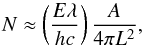 (1)where E ≈ 109−1010 J is the emitted optical energy, λ ≈ 656.28 nm is the dominant wavelength of the emissions, A = 73 m2 is the collecting area of the telescope, L ≈ 5 AU is the Earth-Jupiter distance, and h,c have their usual meaning. These quantities lead to N ≈ 4 × 10⁴ to 4 × 10⁵ photons at the detector. This number suggests that lightning can be plausibly detected, which was our motivation to attempt the detection of Jovian flashes from the Gran Telescopio de Canarias (GTC).
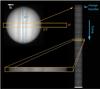 |
Fig. 1 Setup of our observations. The slit had a field of view of 2.5′ × 3′′ and was aligned along Jupiter’s polar axis. During the observation Jupiter had a visible diameter of about 41′. The slit was open during 50 ms, and after the exposure, the CCD charges were transferred to lower pixels, thus forming the stripe pattern image shown on the right. Each image consisted of 58 valid stripes, and we collected 208 images. For clarity, lengths in the picture are not to scale. |
2. Methods
Our observations were made on 14 March 2014, using the fast-photometry mode of GTC combined with the red tunable filter (RTF). Our setup is summarized in Fig. 1. The fast-photometry mask of OSIRIS covers a field of view (FOV) of 7′ × 3′′, but we windowed the CCD readout and used a FOV of only 2.5′ × 3′′, a window 1200 pixels wide. The center of the Jupiter disk was located at 2.78′′ from the CCD center, and the RTF was set to a central wavelength of 660.2 nm, and the minimum achievable width of 1.2 nm was used. The effective wavelength at which the RTF filter is tuned varies along the CCD. With this setup, the central wavelength was set to 656.3 nm (Hα line) in the center of the Jupiter disk. Given the angular size of Jupiter, the changes in this central wavelength are ±0.34 nm from pole to pole (the north pole being redder than the south pole). This change in wavelength is much smaller than the width of the filter. Over the sky area, the central wavelength of the RTF changes as well, but here the expected contribution is only that of cosmic rays impacting the detector, which is not wavelength sensitive.
Using the model spectra of Borucki et al. (1996) as a reference, we estimated the power fraction of the optical energy that passes through our filter. Assuming perfect transmission inside a window of 1.2 nm around 656.28 nm and no transmission outside, we estimate that we collected 3%−5% of the light from a lightning flash reaching the telescope, depending on whether the lightning originated at 5 bar or 1 bar. Following Dyudina et al. (2004), we consider the highest pressure more likely and therefore assumed a transmission rate T = 3% for our setup.
At the time of our observation, Jupiter was at about 4.85 AU, with an apparent diameter of 40.6′′. At that distance, lightning on a scale of 100 km subtends an angle of about 0.03′′; our signal-to-noise ratio would be highest at this angular resolution, but we were limited by the OSIRIS resolution of about 0.254′′ and, more importantly, by the natural seeing of about 1′′ (see below).
According to Borucki et al. (1996), the best signal-to-noise ratio is obtained when the selected exposure time is equal to the duration of a lightning flash. In our setup, individual exposure times were 50 ms, after which the charge was transferred to lower pixels in less than 1 ms. Shorter exposure times would have been desirable, but cannot be achieved with OSIRIS. Up to 58 valid subimages were obtained before the CCD was full and had to be readout in 18 s. We refer to each of these subimages as a frame, while the set of 58 consecutive frames obtained in a CCD readout is called a series. In total, 208 series (each with 58 frames) were collected, totalling 12 064 frames, which is equivalent to a total exposure time of 603.2 s.
Immediately after recording these data, we captured images of a distant star (55 Canc, Mv = 5.95) that we used to measure our seeing conditions. From these images we estimate that the maximum of the normalized point spread function (PSF) is about α = 0.015, meaning that a point source with a total intensity I produces a peak pixel intensity of about 0.015I.
Taking into account this smearing out and the fraction of light transmitted by our filter, our estimate of about 4 × 10⁴ to 4 × 10⁵ photons per flash collected by the telescope translates into a peak of between 18 and 180 photon counts. In general, and returning to (1) but accounting for the filter transmittance and smearing-out, an event with a peak count rate Ip corresponds to an optical energy at the source E = 4πhcL2Ip/λαAT ≈ Ip × (6.1 × 10⁷ J).
3. Data analysis
3.1. Statistical distribution of intensity fluctuations
Since the rotation of Jupiter and the displacement of cloud features in the planet have characteristic times much longer than the interval between two consecutive frames, the variations between frames whithin a single series may only be due to one of the following factors:
-
1.
Shot noise from the telescope’s CCD. Sometimes called photon noise, this refers to variations in the random arrival of photons to our detector. We neglect other forms of noise such as readout noise, which in OSIRIS is below 4.5 counts per pixel (Cabrera-Lavers 2013).
-
2.
Variations in the terrestrial atmosphere, seen as temporal variations in the transmittance that equally affect all pixels, but also changes in the PSF that distort the geometry of the cloud features in Jupiter.
-
3.
Spurious signals due to the incidence of a cosmic ray into the CCD during the exposure or readout time.
-
4.
Lightning flashes or any other transient event occuring in the Jovian atmosphere.
We adopt here the null hypothesis that the data can be explained by factors 1−3 alone, which means that there is no statistically significant detection of lightning flashes. To reach this conclusion, we first need to analyze the signal expected from each of the items above.
We first investigate the broad statistical features of our sample. Since each of the 208 series of frames (subexposures) was analyzed independently, we focus on one of them. Let Ii,j be the signal measured at pixel i in frame j, where 1 ≤ i ≤ M, 1 ≤ j ≤ N, with M = 1200 × 19 = 22 800 being the number of pixels in each subexposure and N = 58 the number of subexposures in each image. Transient events cause variations of Ii,j relative to the frames immediately preceding and following j, which we quantify as 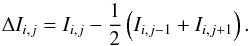 (2)This value is clearly undefined for the first and last frames in a series, which are not used here.
We collected all the values of ΔI in the observation and separated them into those within the sensor area illuminated by the planet and those in the region exposed only to the dark sky. The empirical distribution functions of each of these collections, normalized to unity, are shown in Fig. 2. The normalization allows us to compare the two distributions even though they result from different areas in the detector. Note that in this analysis we ignored the spatial distribution of the ΔI, that is, if a single cosmic ray left a mark in several pixels, we counted each of them individually.
The distribution from inside the planet consists of a large bulk followed by a power-law tail, with the transition between them being around ΔI ≈ 1500 counts (corresponding to about 8.2 × 10¹⁰ J optical energy at the source). The bulk, which is obviously absent from the sky distribution, contains the intensity variations due to shot noise entangled with variations in the atmospheric conditions (i.e., points 1 and 2 above). The tail, on the other hand, is very similar in the planet and the sky distributions. This suggests that these ΔI are unrelated to any process in Jupiter, but instead result from cosmic rays impacting the sensor (i.e., point 3 in the previous list).
Even though in this preliminary visual inspection of Fig. 2 we do not see any feature that deviates from the null hypothesis, it is still possible that a weak signal is hidden behind the noise and the artifacts that dominate the distribution. To rule out this possibility, we now engage in a more precise statistical analysis.
3.2. Cosmic-ray tail
We first consider the tails of the two distributions in Fig. 2. In principle, a difference in these two distributions would indicate energetic, transient emissions in Jupiter. However, we must be careful: even if these emissions do not exist, there would still be a slight difference in the tail distributions of the clear sky and the planet. The reason is that inside the planet the counts produced by each cosmic ray are added to the background noise, which is much higher than in the sky.
Therefore, to rule out any contribution of transient emissions from Jupiter, we compared the tail distribution of the planet with an artificial distribution derived from the sky data. We constructed this distribution by adding to each ΔI value in the sky sector a randomly chosen ΔI from within the planet. Neglecting the low probability that the chosen ΔI corresponds to a cosmic ray, the resulting distribution is what we would expect from inside the planet in the absence of lightning flashes. Limiting ourselves to ΔI> 1500, we applied a Kolmogorov-Smirnov test to the data from inside the planet and the artificial distribution. The resulting p-value of 0.3 is consistent with both distributions being identical, therefore we conclude that there is no statistically significant presence of flashes in the tail of the distribution.
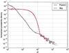 |
Fig. 2 Histogram of occurrences of values of ΔI for the detector area exposed to the planet and for the area exposed to the dark sky. |
3.3. Bulk of the distribution
After excluding lightning flashes in the tail of Fig. 2, we may still wonder whether there are flashes hidden within the bulk of the histogram. To address this possibility, we return to our list of possible causes of variation and explore how the bulk distribution is determined by items 1 and 2.
The shot noise in the number of photons reaching a pixel in the CCD follows a Poisson distribution. If the gain of the CCD is g = 1, the probability that the signal in a given pixel equals I is  (3)where μ is the expected value of I, uniquely characterizing the distribution. In general, μ depends on the pixel location i and the frame index j, but for clarity we have omitted the indices here. For a general g, the Poisson distribution applies not to the signal I, but to the number of photons collected by the CCD, gI:
  (4)The OSIRIS user manual (Cabrera-Lavers 2013) estimates g ≈ 0.90 for the CCD we used. However, since our measurements are very sensitive to small deviations in g, we describe below how we fitted g to minimize deviations from our data.
To test (4) against our observations, we need a good estimation of the expected value μ. If μ were independent of the frame j, we could have estimated it by averaging Iij over j. However, μ may be different between different exposures for a given pixel due to the variations in the atmospheric transmittance and PSF.
We thus arrive at the central point of our analysis: how to distinguish the shot noise from the random variations introduced by the atmosphere, given that we do not have an accurate model for the latter. The key here is that the variations caused by the atmosphere are strongly correlated between different pixels, whereas shot noise is uncorrelated. Therefore we can isolate the shot noise by removing from the variations in one pixel the part that is correlated with other pixels in the image.
We used the principal component analysis (PCA; Jolliffe 2002) to perform this separation. With this technique we decomposed the signal Iij as Iij = μij + rij where the μij, although different for each pixel, are heavily correlated and estimate the signal expected in the absence of noise. The shot noise is thus contained in the residua rij, which are mostly uncorrelated. In our analysis we obtained μij by projecting Iij into the subspace defined by its three first components.
As in any attempt to extract a signal from noisy data, we cannot avoid some amount of overfitting. In our case, this means that the expected values μij, because they result from a fit of the measured intensity, follow the data too closely and therefore underestimate the noise, ideally contained in rij. However, using a bootstraping method, we checked that the rij arise from shot noise by comparing their distribution with the distribution of random variables  that we sampled as follows: after obtaining μij, use them as parameters of a Poisson distribution to generate a new set of random
  ; then apply the PCA over these random intensities to obtain
  and such that
  . By construction, the result purely from Poissonian noise; by comparing the distributions of rij and we can find out if the rij can also be explained purely by noise. Note that although μij and are different, both derive from averaging over many data points, so their difference is much smaller than the noise.
However, note that the distribution of the new depends on the detector gain g, which we do not know precisely. Given the large number of sample points that we accumulated, even small deviations from the precise value of g cause statistically significant differences in the distributions of r and r′. To exclude that possibility, we searched for the g that minimizes the Kolmogorov-Smirnov distance between the two samples, including the full set of measurements. This was achieved for g ≈ 0.9118, close to the value g ≈ 0.9 provided by the OSIRIS manual (Cabrera-Lavers 2013). For this value we obtained a p-value of about 0.6, which is consistent with r and r′ being equally distributed and hence with the null hypothesis that r only contains noise.
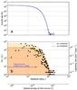 |
Fig. 3 a) Histogram of the residuals r after performing a principal components analysis to remove atmospheric variations. The residuals are distributed among equally spaced bins of width w = 10. b) Difference between the counts per bin in our data, nb and in a randomly generated sample that simulates shot noise, |

3.4. Detection threshold
The separation between noise and atmospheric variation enables us to quantify our detection threshold. We distributed the values of rij for all images and subexposures within equally spaced bins of width w = 10; the resulting histogram is plotted in Fig. 3a. The number of residues r falling into a bin b is nb. How large must nb be to distinguish it from random variations? We can estimate this threshold by comparing nb with  , the number of values from the purely random sample r′ that fell into the same bin. If nb is random, the variance of the difference
  is
is  (5)where the latter approximate equality arises because the number of events inside a bin is again Poisson-distributed.
To claim a significant deviation from randomness, the magnitude of the difference  must therefore be larger than a few times the standard deviation
  . In Fig. 3b we plot σ and 3σ together with the measured
  . Clearly, we lack a significant signal above the random background except in the cosmic-ray tail, which we have already discarded.
Since the σ and 3σ curves in Fig. 3b quantify the background noise of our observations, they also mark the detectability threshold and thus constrain the occurrence of flashes in Jupiter. For this reason, on the right vertical axis we translated these values into counts per square kilometer per year, assuming a constant and homogeneous distribution of flashes. Here we took into account the total observation time and the area of Jupiter covered by the slit. In principle, our results show that for a given excess intensity r, the number of flashes per second in Jupiter is below the 3σ curve: otherwise we would have observed them. However, note that this analysis does not account for the clustering of flashes in space or in time.
4. Discussion and conclusions
Although unsuccessful, our search may be useful for future investigations. The lowest horizontal axes in Fig. 3b measure the optical energy corresponding to a given count excess, where we have accounted for smearing and filter transmission. As we mentioned above, a strong flash in Jupiter would emit an optical energy of about 1010 J, leaving about 180 counts in our CCD. At about this value, our setup required at least some thousands of events per bin to distinguish them from noise. This number of flashes within our observation time corresponds to a flash rate of a few times 1 km-2 yr-1, far above the estimate of 4.2 × 10⁻³ km-2 yr-1 reported by Little et al. (1999). On the other hand, Fig. 3b shows that even a few flashes with energies around 1011 J would have been enough to distinguish them from cosmic rays; these energies are significantly above the maximum energy observed by in-situ spacecraft, however.
Our research, and in particular Fig. 3b, suggest several possible ways to increase the chances for detecting Jovian lightning from a ground-based telescope:
-
1.
The first way is to accumulate more observation time to increasethe signal-to-noise ratio. A short consideration shows thisapproach to be unrealistic: considering the rate estimated byLittle et al. (1999), we would needto improve our signal-to-noise ratio by a factor ofabout 103 to detect flashes of 109 J. This would entail increasing our observation time by a factor 106, which is obviously impossible.
-
A more promising approach would be to increase the peak pixel signal that a flash leaves in the CCD. As we said above, the atmosphere smeared out our signal by a factor α = 0.015; without that distortion, a 109 J-flash would create a signal of about 103 counts, where the curve of Fig. 3b moves below the expected rate, facilitating a detection. Reducing the atmospheric distortion can be accomplished with adaptive optics (AO), which would bring our resolution closer to the resolution limit of the telescope (0.254′′ for OSIRIS). This technique is not yet available at GTC, however.
-
3.
A complementary method to improve our detection threshold is to consider the clustering of lighting flashes. By mapping pixels to planet coordinates, we can search for regions that accumulate several high pixel values. This technique by itself is not enough within our setup: the number of candidate events detected with intensities corresponding for instance to a 1010 J-flash is still too large to detect patterns indicating a thunderstorm.
We finally note that the strongest barrier for our observation was the intense sunlight scattered by Jupiter. Observing a planet with part of its night-side facing Earth would strongly reduce the background noise, lowering the detection threshold. The only suitable candidate for this is Venus, and, as we mentioned in the introduction, these observations were carried out by Hansell et al. (1995) but have not been reproduced afterwards (Yair 2012).
As this preliminary work shows, although extraterrestrial lightning is intense enough to be detected from ground-based telescopes, it is very difficult to distinguish this signal from scattered sunlight in the dayside of external planets. However, the improved instrumentation and larger telescopes that will become available within the next decade offer a realistic chance of success in these observations. It is our hope that this work will provide a basis for future investigations in this direction.
Acknowledgments
A.L. and F.J.G.V. were supported by the Spanish Ministry of Economy and Competitiveness (MINECO) under projects AYA2011-29936-C05-02 and ESP2013-48032-C5-5-R and by the Junta de Andalucía, Proyecto de Excelencia FQM-5965. E.P. was supported by the MINECO ESP2013-48391-C4-2-R grant. Based on observations made with the Gran Telescopio Canarias (GTC), instaled in the Spanish Observatorio del Roque de los Muchachos of the Instituto de Astrofísica de Canarias, in the island of La Palma.
References
- Baines, K. H., Simon-Miller, A. A., Orton, G. S., et al. 2007, Science, 318, 226 [NASA ADS] [CrossRef] [Google Scholar]
- Borucki, W. J., McKay, C. P., Jebens, D., Lakkaraju, H. S., & Vanajakshi, C. T. 1996, Icarus, 123, 336 [NASA ADS] [CrossRef] [Google Scholar]
- Cabrera-Lavers, A. 2013, OSIRIS User Manual v3.1, Tech. rep., http://www.gtc.iac.es/instruments/osiris/media/OSIRIS-USER-MANUAL_v3_1.pdf [Google Scholar]
- Cook, II, A. F., Duxbury, T. C., & Hunt, G. E. 1979, Nature, 280, 794 [NASA ADS] [CrossRef] [Google Scholar]
- Dyudina, U. A., Ingersoll, A. P., Ewald, S. P., et al. 2010, Geophys. Res. Lett., 37, 9205 [Google Scholar]
- Dyudina, U. A., Ingersoll, A. P., Ewald, S. P., et al. 2013, Icarus, 226, 1020 [NASA ADS] [CrossRef] [Google Scholar]
- Dyudina, U. A., Del Genio, A. D., Ingersoll, A. P., et al. 2004, Icarus, 172, 24 [NASA ADS] [CrossRef] [Google Scholar]
- Fischer, G., Gurnett, D. A., Kurth, W. S., et al. 2008, Space Sci. Rev., 137, 271 [NASA ADS] [CrossRef] [Google Scholar]
- Gurnett, D. A., Shaw, R. R., Anderson, R. R., & Kurth, W. S. 1979, Geophys. Res. Lett., 6, 511 [NASA ADS] [CrossRef] [Google Scholar]
- Gurnett, D. A., Kurth, W. S., Cairns, I. H., & Granroth, L. J. 1990, J. Geophys. Res., 95, 20967 [NASA ADS] [CrossRef] [Google Scholar]
- Gurnett, D. A., Kurth, W. S., Roux, A., et al. 1991, Science, 253, 1522 [NASA ADS] [CrossRef] [Google Scholar]
- Hansell, S. A., Wells, W. K., & Hunten, D. M. 1995, Icarus, 117, 345 [NASA ADS] [CrossRef] [Google Scholar]
- Jolliffe, I. 2002, Principal Component Analysis, Springer Series in Statistics (New York, USA: Springer-Verlag) [Google Scholar]
- Kaiser, M. L., Desch, M. D., Farrell, W. M., & Zarka, P. 1991, J. Geophys. Res., 96, 19043 [NASA ADS] [CrossRef] [Google Scholar]
- LeBlanc, F., Aplin, K., Yair, Y., et al. 2008, Planetary Atmospheric Electricity, 1st edn. (Springer Publishing Company, Incorporated) [Google Scholar]
- Little, B., Anger, C. D., Ingersoll, A. P., et al. 1999, Icarus, 142, 306 [NASA ADS] [CrossRef] [Google Scholar]
- Magalhaes, J. A., & Borucki, W. J. 1991, Nature, 349, 311 [NASA ADS] [CrossRef] [Google Scholar]
- Porco, C. C., West, R. A., Squyres, S., et al. 2004, Space Sci. Rev., 115, 363 [NASA ADS] [CrossRef] [Google Scholar]
- Warwick, J. W., Pearce, J. B., Evans, D. R., et al. 1981, Science, 212, 239 [NASA ADS] [CrossRef] [PubMed] [Google Scholar]
- Yair, Y. 2012, Adv. Space Res., 50, 293 [NASA ADS] [CrossRef] [Google Scholar]
- Zakharenko, V., Mylostna, C., Konovalenko, A., et al. 2012, Planet. Space Sci., 61, 53 [NASA ADS] [CrossRef] [Google Scholar]
- Zarka, P., & Pedersen, B. M. 1986, Nature, 323, 605 [NASA ADS] [CrossRef] [Google Scholar]
All Figures
|
Fig. 1 Setup of our observations. The slit had a field of view of 2.5′ × 3′′ and was aligned along Jupiter’s polar axis. During the observation Jupiter had a visible diameter of about 41′. The slit was open during 50 ms, and after the exposure, the CCD charges were transferred to lower pixels, thus forming the stripe pattern image shown on the right. Each image consisted of 58 valid stripes, and we collected 208 images. For clarity, lengths in the picture are not to scale. |
| In the text | |
|
Fig. 2 Histogram of occurrences of values of ΔI for the detector area exposed to the planet and for the area exposed to the dark sky. |
| In the text | |
|
Fig. 3 a) Histogram of the residuals r after performing a principal components analysis to remove atmospheric variations. The residuals are distributed among equally spaced bins of width w = 10. b) Difference between the counts per bin in our data, nb and in a randomly generated sample that simulates shot noise, |
| In the text | |
Current usage metrics show cumulative count of Article Views (full-text article views including HTML views, PDF and ePub downloads, according to the available data) and Abstracts Views on Vision4Press platform.
Data correspond to usage on the plateform after 2015. The current usage metrics is available 48-96 hours after online publication and is updated daily on week days.
Initial download of the metrics may take a while.