| Issue |
A&A
Volume 577, May 2015
|
|
|---|---|---|
| Article Number | A34 | |
| Number of page(s) | 9 | |
| Section | The Sun | |
| DOI | https://doi.org/10.1051/0004-6361/201425387 | |
| Published online | 27 April 2015 | |
Visible light and ultraviolet observations of coronal structures: physical properties of an equatorial streamer and modelling of the F corona
INAF–Catania Astrophysical Observatory,
95123
Catania,
Italy
e-mail:
This email address is being protected from spambots. You need JavaScript enabled to view it.
Received: 21 November 2014
Accepted: 25 February 2015
Abstract
The present work studies the characteristics of an equatorial streamer visible above the east limb of the Sun on March 2008, during the most recent minimum of solar activity. We analysed the visible light coronagraphic images of SOHO/LASCO and the ultraviolet observations in the H I Lyα spectral line obtained by SOHO/UVCS, and exploited the Doppler dimming effect of the coronal Lyα line to derive the outflow velocity profile of the scattering neutral hydrogen atoms in the streamer region. Taking advantage of the synergy between visible light and ultraviolet observations, we were able to determine all the properties of the coronal structure. In particular, the actual extent of the streamer along the line of sight has been evaluated for the first time. In so doing, the solar wind outflow velocity turned out to be the only free parameter in the theoretical modelling of the Lyα intensity. We found nearly static conditions below 3.5 R⊙ along the streamer axis, whereas the solar wind flows at velocities from 40 km s-1 to 140 km s-1 in the altitude range 2.5–5.0 R⊙ along the southern boundary of the streamer. We also derived the intensity distribution of the F coronal component in the LASCO C2 field of view, by combining total and polarized brightness data. Finally, we investigated the dependence of the Lyα resonant scattering process on the kinetic temperature of the coronal neutral hydrogen atoms and found that the value of this temperature mostly affects the scattering process at low heliocentric distances, where the solar wind flows with low velocity.
Key words: Sun: corona / solar wind / Sun: UV radiation
© ESO, 2015
1. Introduction
Coronal streamers are quasi-stationary large-scale structures that are thought to be associated with underlying active regions and/or prominences. They are likely to be the result of a complex interaction between the surrounding solar wind and the large-scale magnetic field. Streamers are impressive near the maximum of the solar cycle, filling the solar corona at almost every latitude, while they are mainly located around the solar equator during minimum, forming the so-called streamer belt.
Streamers are tenuous structures with respect to the solar photosphere, and this made their early observations possible only during total solar eclipses. In the past decades, the ceaseless monitoring of the coronal features through the visible light (VL) images of the Large Angle and Spectrometric COronagraph (LASCO; Brueckner et al. 1995), the ultraviolet (UV) observations of the UltraViolet Coronagraph Spectrometer (UVCS; Kohl et al. 1995) onboard the SOlar and Heliospheric Observatory (SOHO; Domingo et al. 1995), and the stereoscopic investigation with the Solar TErrestrial RElations Observatory (STEREO; Kaiser et al. 2008) has significantly contributed to augmenting the knowledge of the physical properties of streamers and to identifying the sources of fast and slow solar winds.
The VL coronagraphic and UV spectrometric observations are usually used to investigate the solar wind at coronal level via the Doppler dimming technique (Hyder & Lytes 1970; Noci et al. 1987; Withbroe et al. 1982). In the regions where the solar wind flows, the emission of the coronal H I Lyα line (121.6 nm) is dimmed, and the dimming depends on the outflow velocity in the expanding corona. Therefore, one can examine how the solar wind flows into the corona and distinguish between fast and slow streams by measuring the intensity of this spectral line.
The scientific goal of the present work is to contribute to the study of the physical properties of coronal streamers, which is crucial for identifying the sources of the slow solar wind. We exploited the Doppler dimming effect of the coronal H I Lyα line to obtain the outflow velocity profile in an equatorial streamer visible on March 2008 by theoretically reproducing the Lyα intensity measured by UVCS.
As for any UV spectral line, the specific intensity of the H I Lyα line depends on the physical parameters of the emitting region. We used visible light polarized brightness images of the LASCO C2 coronagraph to derive some of them, such as electron density and temperature, and the extent of the streamer along the line of sight (LOS). We also determined the specific intensity of the coronal Lyα line from the contemporaneous spectrometric observations of UVCS and derived the kinetic temperature of the H I scattering atoms from the Doppler line broadening. In so doing, the solar wind outflow velocity turns out to be the only free parameter in the theoretical modelling of the Lyα intensity for the first time. It is worthwhile noting that in the past the extent of the streamer along the LOS has just been assumed (see Spadaro et al. 2007; Susino et al. 2008).
In addition, we provide an estimate of the contribution of the Fraunhofer corona (F corona) to the total visible emission by combining LASCO C2 data of total and polarized brightness. The visible light total brightness is mainly due to the emission of the Kontinuierlich corona (K corona), arising from the Thomson scattering of photospheric light by free coronal electrons, and of the F corona. The F corona is defined as the coronal component due to the scattering of photospheric light by the interplanetary dust, and it must be removed when measuring the intensity of Thomson-scattered radiation. Our aim is to evaluate an alternative to the use of an empirical F-corona model, when the total and polarized brightness can be simultaneously known.
In this context, we also assess the possibility of performing the present study by using the forthcoming instrument METIS (Antonucci et al. 2012), a coronagraph selected by the European Space Agency (ESA) for the scientific payload of the Solar Orbiter mission (Müller et al. 2013). Solar Orbiter, whose launch is scheduled in July 2017, is dedicated to investigating the linking of solar atmosphere phenomena to their evolution in the inner heliosphere. METIS will provide simultaneous imaging of the full corona from 1.6 to 5.5 R⊙, in total and polarized visible light, and in the H I Lyα line. However, it was not conceived to provide line profiles, and it does not allow a direct determination of the kinetic temperature of the scattering neutral hydrogen atoms in the corona. This induced us to investigate how the Lyα scattering process in corona depends on the value of kinetic temperature.
2. Coronal H I Lyα intensity
The emission of the coronal H I Lyα line is mainly due to two mechanisms: 1) collisional excitation by free electrons impact and 2) resonant scattering of chromospheric photons by neutral hydrogen atoms, with the first one accounting for only a small fraction of the total intensity of the radiative process (Gabriel 1971; Raymond et al. 1997). Resonant scattering of the solar chromospheric light by neutral hydrogen atoms thus becomes the primary tool for studying the corona at 121.6 nm. The intensity of the resonantly scattered component of the H I Lyα line depends directly upon the emitting source, but it is also sensitive to the speed of the coronal plasma, and this introduces the possibility of using the Doppler dimming effect to measure the outflow velocity of the solar wind.
An expression for the total intensity IS of the Lyα scattered radiation can be deduced as in Withbroe et al. (1982). Here we follow a simpler approach that allows us to compute the total scattered intensity, neglecting the determination of the Lyα line profile. The geometry of the scattering process and the adopted notation are illustrated in Fig. 1 (see e.g. Noci & Maccari 1999). If j(P,n) is the coronal emissivity in a point P where a chromospheric Lyα photon, moving in the direction n′, is absorbed by a hydrogen atom with velocity v and re-emitted in the direction n, we have 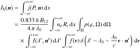 (1)where x is the direction along the LOS, c the light speed, h the Planck constant, B12 the Einstein coefficient related to the transition with central wavelength λ0, ne the electron density, Ri the neutral hydrogen fraction (function of the electron temperature), and Ω the solid angle under which the point P subtends the solar disk. The geometric factor p(ϕ,Ω) = [ 11 + 3(n·n′)2 ] /12 represents the probability that the absorbed photon, coming from the direction n′, will be scattered through the angle ϕ in the direction n, and I(λ′,n′) is the specific intensity of the chromospheric profile. Moreover, f(v) is the velocity distribution function of the coronal hydrogen atoms (function of the kinetic temperature), and the Dirac delta function takes into account that the chromospheric photons incident on P from different directions n′ within the solid angle Ω that can be scattered by coronal atoms with velocity v are those with
  .
.
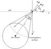 |
Fig. 1 Adopted geometry for the resonant scattering process in the coronal point P. The Cartesian y-axis points outwards from the plane of the page. |
If a Maxwellian velocity distribution is adopted for the scattering atoms, the last integral in Eq. (1)can be analytically solved. By using the xyz right-handed coordinate system of Fig. 1, the expression for IS(n) can also be numerically integrated, and in particular, one obtains n·n′ = cosϕ and v·n′ = vwcos(φc − ϕ) + vn′, where vw is the solar wind outflow velocity, φc is the angle between the directions of vw and n, and vn′ is the component of the thermal speed of the hydrogen atom in the direction n′. We assumed uniform chromospheric intensity and used the analytical form of the profile proposed by Auchère (2005); it is a sum of three Gaussians and has the following expression: ![Mathematical equation: \begin{equation} I(\lambda^\prime,\vec{n^\prime})=I(\lambda^\prime)=I_\mathrm{t}\displaystyle\sum_{i=1}^{3}\,\left[\frac{a_{i}}{\sigma_{i}\sqrt{\pi}}{\rm e}^{-(\lambda^\prime-\lambda_\mathrm{0}-\delta\lambda^\prime_{i})^2/\sigma_{i}^2}\right] \label{gaussians} \end{equation}](/articles/aa/full_html/2015/05/aa25387-14/aa25387-14-eq31.png) (2)where It is the total intensity of an elementary surface of the chromosphere. The assumption of uniform intensity of the solar disk is valid when investigating Lyα radiation coming from the coronal region near equatorial latitudes (Auchère 2005), and it allows us to neglect the dependence on the solid angle Ω of the chromospheric specific intensity. Measurements of H I outflow velocity via the Doppler dimming effect depend directly on the value of chromospheric Lyα intensity, which varies by a factor of about 1.8 through the solar cycle (Woods et al. 2000). From the sets of irradiance measurements carried out by Lemaire et al. (2002) at solar minimum, we obtained It = 105 erg cm-2 s-1 sr-1. The values of ai, σi, e
(2)where It is the total intensity of an elementary surface of the chromosphere. The assumption of uniform intensity of the solar disk is valid when investigating Lyα radiation coming from the coronal region near equatorial latitudes (Auchère 2005), and it allows us to neglect the dependence on the solid angle Ω of the chromospheric specific intensity. Measurements of H I outflow velocity via the Doppler dimming effect depend directly on the value of chromospheric Lyα intensity, which varies by a factor of about 1.8 through the solar cycle (Woods et al. 2000). From the sets of irradiance measurements carried out by Lemaire et al. (2002) at solar minimum, we obtained It = 105 erg cm-2 s-1 sr-1. The values of ai, σi, e  in Eq. (2)are reported in Auchère (2005), and the computed profile is shown in Fig. 2.
In this work we used the theoretical expression reported in Eq. (1)to reproduce the intensity of the resonantly scattered component of the coronal H I Lyα line measured by UVCS, during observations of an equatorial streamer visible on March 2008. Our purpose was to derive the outflow velocity of the scattering atoms at different heliocentric distances in the streamer region, by iteratively reproducing the set of observational results as closely as possible. Equation (1)can be solved after determining all the physical properties of the streamer. We used LASCO C2 data to estimate the electron density and temperature, and the extent along the LOS of the coronal structure. In addition, we exploited the information on the Lyα line profile obtained by UVCS to determine the velocity distribution function f(v) of the neutral hydrogen atoms, assuming an isotropic Maxwellian distribution.
3. Observations
We studied the physical properties of an equatorial streamer during the most recent minimum phase of the solar cycle, taking advantage of synergy of visible light and ultraviolet observations. We used UV spectral data collected during investigation of coronal dynamics and outflow velocity carried out by UVCS in 2008 from March 10 at 17:34 UT to March 11 at 17:47 UT. The spectrometric observations consist of radial scans of the streamer at 1.77, 2.53, 3.03, 4.03, and 5.03 R⊙ above the eastern limb of the Sun in the 70°–130° range of polar angle (PA, measured counterclockwise from solar north pole). Specific intensities of the H I Lyα spectral line have been measured by UVCS with a spatial binning of eight pixels, giving a spatial resolution of 56 arcsec (7 arcsec per pixel) along a 40 arcmin entrance slit. The slit width has been set equal to 50 μm at 1.77, 2.53, 3.03 R⊙, and to 102 μm at 4.03 and 5.03 R⊙, in order to optimize both spectral resolution and photon flux. The exposure time was 200 s in all cases, and the number of exposures was chosen for each position of the entrance slit so as to optimize the signal-to-noise ratio. Owing to the on-orbit degradation of the performance of the UVCS detector with time, we were able to determine the Lyα intensity at the slit positions only along two radial paths: at 85° PA, which corresponds to the streamer axis on the plane of the sky (POS), and 95° PA, which outlines the southern boundary of the streamer.
The streamer has also been observed by LASCO C2 in visible light total (B) and polarized brightness (pB). During the time interval of the UVCS observations, LASCO provided total brightness images with about a 20-min time cadence and four pB images. Thanks to the quiescent condition of the solar corona, we only considered the pB image taken at 9:00 UT on March 11, 2008. Figure 3 reports the instantaneous positions of the UVCS slit during the radial scans in the LASCO C2 field of view (FOV), which ranges from 2.5 to 6.5 R⊙.
 |
Fig. 3 LASCO C2 pB image taken at 9:00 UT on March 11, 2008, and UVCS slit positions at 1.77, 2.53, 3.03, 4.03, and 5.03 R⊙ above the east limb of the Sun. The dotted lines indicate the two radial paths along which we were able to determine the Lyα intensity from the UVCS observations. The dash-dotted line outlines the limb of the solar disk. |
4. VL data analysis
4.1. Physical parameter estimate
Visible light observations are typically used to derive the radial electron density profile in the corona. Van De Hulst (1950) developed a method based on the inversion of the pB intensity in order to determine the coronal electron density ne as a function of the heliocentric distance r, according to the following formula (Billings 1966; Hayes et al. 2001; Van De Hulst 1950): ![Mathematical equation: \begin{equation} pB(x)=C\!\displaystyle\int_{x}^{\infty}\!\!\!\!n_\mathrm{e}(r)\,[\mathcal{A}(r)-\mathcal{B}(r)]\frac{x^2}{r\sqrt{r^2-x^2}}\,\mathrm{d}r \label{pb} \end{equation}](/articles/aa/full_html/2015/05/aa25387-14/aa25387-14-eq42.png) (3)where C is a conversion factor,
(3)where C is a conversion factor,  and ℬ are geometric factors (Billings 1966; Van De Hulst 1950), and x is the projected distance on the POS.
The radial profiles are usually computed on the hypothesis that the electron density is symmetric with respect to the POS along the LOS. We also assumed that the radial electron density profiles can be expressed by the polynomial form ne(r) = ∑ k(αkr− k), as described in Hayes et al. (2001). Then we substituted the expression of ne(r) in Eq. (3), with k varying between 1 and 4 in order to avoid the unwanted instabilities common to high-degree polynomial fits and used a multivariate least-squares fit of the resulting equation to obtain the coefficients αk that best reproduce the pB intensity of the LASCO C2 image. These coefficients were substituted into the polynomial form of the electron density to derive the radial density profiles for the full LASCO C2 FOV. Figure 4 reports the resulting profiles in the streamer region from 80° to 100° PA (one dotted line for each degree), and, for comparison, the average profile calculated by Gibson et al. (1999), who modelled the electron density of a streamer at solar minimum. Both results have been obtained by the inversion method of pB data, and they show very good agreement in the altitude range from 2.5 to 6.2 R⊙. We also took the fraction of polarization p of the F corona in the density calculations into account. This contribution is negligible at low heliocentric distances (Mann 1992), but can become significant at higher distances and should be removed from the pB data when observing the extended corona. Within the LASCO C2 FOV, p is about zero for r< 4.95R⊙, whereas it is given by p = 0.0067 r−0.0332 for r = 4.95–6.0 R⊙ and by p = 0.009 r−0.047 for r> 6.0R⊙ (see Koutchmy & Lamy 1985). We computed the polynomial fits of the coronal electron density values by first removing the fraction of polarization of the F corona from the pB data and then not doing so, and found an average variation in the density profiles of about 4%. Our results also agree with those obtained through the inversion method by Spadaro et al. (2007) and Susino et al. (2008), who studied the physical properties of a mid-latitude quiescent streamer visible on May 2004, whereas the median density solutions calculated by Frazin et al. (2003) and Strachan et al. (2002) along the streamer axis are higher by a factor of about 2. Antonucci et al. (2005) determined average coronal electron densities from the analysis of the OVI resonance doublet and found ne = (8.5 ± 0.6) × 105 cm-3 at 2.3 R⊙ and ne = (3.3 ± 0.6) × 105 cm-3 at 3.5 R⊙ within the region of their streamer, and ne = (1.8 ± 0.3) × 105 cm-3 and ne = (7.0 ± 1.8) × 104 cm-3 at the same altitudes out of the streamer. These values agree with ours.
 |
Fig. 4 Radial electron density profiles computed in the streamer region from 80° to 100° PA (dotted lines), while the solid line indicates, for comparison, the profile calculated by Gibson et al. (1999). The radial electron density profiles obtained at 85° PA (dashed line) and 95° PA (dash-dotted line) are shown. |
Once the electron density had been derived, we deduced the electron temperature Te. We assumed a balance between thermal pressure and gravity in an ideal coronal plasma, as described in Gibson et al. (1999). This can be reasonably applied when the outflow speed is well below the sound speed (about 150 km s-1 for a coronal plasma at 1 MK, see e.g. Priest 1987), so that the wind velocity is a minor term in force balance. The assumption of hydrostatic equilibrium only holds at heliocentric distances below 3.5–4.5 R⊙, depending on the PA of the considered radial profiles, while at greater heights the high outflow velocity determined in this study should be considered in force balance (see also the discussion at the end of Sect. 5). In this case, therefore, the values of electron temperature deduced from the electron density, according to Gibson et al. (1999), are only a first approximation estimate. Figure 5 shows the empirical profiles of Te calculated from 80° to 100° PA (one dotted line for each degree), between 2.5 and 6.2 R⊙, and, for comparison, the profile (solid line) deduced by Gibson et al. (1999). These results agree with the Te profiles found by Spadaro et al. (2007) and Susino et al. (2008) and are consistent at 2.7 R⊙ with the value obtained by Fineschi et al. (1998), Te = (1.1 ± 0.3) × 106 K, who measured the profile of the electron scattered H I Lyα line in an equatorial streamer by UVCS. The values of Te are then used to determine the neutral hydrogen fraction Ri, which is in turn used to compute the H I outflow velocity through the Doppler dimming effect.
To reproduce the intensity of the coronal H I Lyα line, as expressed by Eq. (1), we need to determine the streamer extent along the LOS. We were able to evaluate this length scale for the first time by using the information on the electron density, again, and developing a method similar to the one discussed by Dolei et al. (2014b). We used the routine calc_cme_mass.pro available in the SolarSoftware library, which calculates the number of electrons providing the intensity in each pixel of the LASCO C2 pB images. The calc_cme_mass.pro routine recalls eltheory.pro, which exploits the Thomson-scattering theory to compute the value of polarized brightness for a single electron as a function of the heliocentric distance (e.g. Minnaert 1930; Van De Hulst 1950). In the optically thin regime, the ratio between the LASCO C2 pB and the pB for a single electron gives the number of electrons along the LOS that provide the LASCO C2 intensity. We obtained the number of electrons for each pixel of the LASCO C2 image and, consequently, the number of electrons per square centimetre (electrons cm-2), i.e. the column density. To derive the extent of the streamer region, we finally considered the different electron density values along a given LOS, as deduced by the radial profiles of Fig. 4. We integrated these densities over increasing distances from the POS until recovering the corresponding column density value previously computed. The resulting distance can be considered as a rough measure of the streamer length scale along the examined LOS. This procedure was repeated for any LOS in order to shape the whole coronal structure, and as an example, Fig. 6 reports the extent at 85° PA as seen from the solar north pole. Our result agrees well with what is assumed by Spadaro et al. (2007) and Susino et al. (2008), who supposed that the bulk of the coronal emission from a streamer is contained within ±0.2–0.3 R⊙ from the POS.
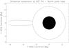 |
Fig. 6 Streamer extent at 85° PA as seen from the solar north pole. The black circle is the Sun, and the dash-dotted line indicates the border of the region hidden from the LASCO C2 occulter. The Cartesian X-axis of the heliocentric Earth equatorial (HEEQ) coordinate system points towards Earth, i.e. towards LASCO. |
4.2. F-corona modelling
The derivation of the coronal electron density from polarized brightness measurements is one of the primary study in solar physics. Actually, total and polarized brightness are complementary; however, B inversion is not a standard method for determining the electron density in corona. The visible light total brightness is mainly due to the emission of the K corona, which arises from the Thomson-scattered radiation, and F corona, owing to the scattered photospheric light by the dust grains. After removing the F corona, stray light, and other spurious contributions, an expression similar to Eq. (3)can be obtained for B as follows (Billings 1966; Hayes et al. 2001; Van De Hulst 1950): ![Mathematical equation: \begin{equation} B(x)=C\!\displaystyle\int_{x}^{\infty}\!\!\!\!n_\mathrm{e}(r)\,\left[\left(\frac{2r^2}{x^2}-1\right)\mathcal{A}(r)+\mathcal{B}(r)\right]\frac{x^2}{r\sqrt{r^2-x^2}}\,\mathrm{d}r \label{tb}. \end{equation}](/articles/aa/full_html/2015/05/aa25387-14/aa25387-14-eq66.png) (4)The lack of a reliable model of F corona precludes the use of total brightness to calculate electron density, even though B is usually much easier to obtain than pB.
(4)The lack of a reliable model of F corona precludes the use of total brightness to calculate electron density, even though B is usually much easier to obtain than pB.
In recent years, several authors have investigated the intensity of the F corona. For instance, Kimura & Mann (1998) discussed the emission of the interplanetary dust in the wavelength range from the visible to the mid-infrared and showed that the hump of the near-infrared brightness at 4 R⊙, sometimes observed in corona, is related to the physical properties of dust grains along the LOS rather than to the existence of a spherical dust ring. The hypothesis of an axisymmetric model of the F corona from the analysis of its morphology and photometry was first proposed by Koutchmy & Lamy (1985); they studied the infrared observations of the dust grains and obtained an expression of the F-corona intensity as a function of the heliocentric distance, which is the most quoted at present. Quémerais & Lamy (2002) used this empirical relationship to remove the dust component from the LASCO total brightness images and obtained the electron density by the inversion method of B. On the other hand, Hayes et al. (2001) also used the technique of the B inversion to derive the electron density profile in the LASCO FOV, without using an empirical F-corona model. They iteratively subtracted a minimum brightness to remove long-lived coronal features and estimate the F-corona contribution; however, their method strongly depends on the specific image, so it must be changed.
We considered the Saito et al. (1977) approach to be a valid method of measuring the intensity of the F corona, under the condition that the electron density depends on the heliocentric distance only radially. Their technique first relies upon determination of the coronal electron density by the pB inversion, according to Eq. (3), to derive a model of K-corona brightness by Eq. (4), which in turn is subtracted from the measured total brightness to obtain the intensity of the F corona. This approach can be easily applied to the visible light data when B and pB are simultaneously known. In the case of LASCO observations, the B images are provided with about 20-min time cadence, while the pB images are taken every six hours. However, we exploited the quiescent condition of the solar corona on March 11, 2008, and used the LASCO C2 total and polarized brightness data obtained at 9:07 and 9:00 UT, respectively. Figure 7 shows the intensity distribution of the F corona in the full FOV of LASCO C2 and some contour levels in units of 1 × 10⁻⁹ mean solar brightness (MSB).
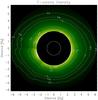 |
Fig. 7 Intensity map of the F-corona in the LASCO C2 FOV, obtained combining the total and polarized brightness taken on March 11, 2008, at 9:07 and 9:00 UT, respectively. The contour levels (dotted lines) are reported in units of 1 × 10⁻⁹ mean solar brightness (MSB). The solid line outlines the limb of the solar disk. |
This illustration induces the following considerations:
-
1.
The brightness distribution appears oblate above2.5 R⊙. In Fig. 8 we report the ellipticity of the intensity distribution, defined as
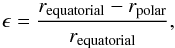 (5)where requatorial and rpolar are the radius vector along the equator (270° PA) and north pole (0° PA) corresponding to an identical F-corona brightness, as a function of requatorial. The profile of the ellipticity is very similar to what is found by Saito et al. (1977), who investigated the equatorial and polar K and F coronal components near solar minimum from the WL coronagraphic data of Skylab (MacQueen et al. 1974).
 -
2.
Contour levels along the streamer region highlight lower intensities than expected at increasing distance. This cannot plausibly be a real feature of the F corona, and it indicates an oversubtraction of the K-corona from the streamer. This is likely due to higher uncertainties in the values of electron density. The radial dependence of the density profile on the heliocentric distance is a good approximation, but it may be a limitation in computing the K coronal component from asymmetric structures, such as streamers (see e.g. Fainshtein et al. 2010; Saito et al. 1977).
Figure 9 shows the profiles of total brightness, K corona, and F corona along the equatorial (90° and 270° PA) and north polar (0° PA) regions. The F-corona profiles obtained by Koutchmy & Lamy (1985) are also reported for comparison. The F corona dominates the K corona, making it difficult to recover the fainter Thomson-scattered radiation (see e.g. Hayes et al. 2001). The F-corona profile computed at 90° PA appears to be less bright than the one calculated by Koutchmy & Lamy (1985), though both profiles exhibit the same slope. However, this difference seems to be comparable to the unexpected decrease in the intensity distribution of the F corona along the streamer region, as shown in Fig. 7. On the other hand, the Koutchmy & Lamy (1985) profile is brighter than the total brightness at 270° PA and lower than what is computed at 0° PA, making it tricky to use the empirical expression in modelling the coronal features with visible light observations.
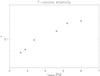 |
Fig. 8 Ellipticity of the F-corona intensity as given by Eq. (5). The plotted points refer to requatorial corresponding to the contour levels reported in Fig. 7. |
In summary, the Saito et al. (1977) method allows the F-corona intensity to be directly determined from visible light observations, when simultaneously measuring total and polarized brightness. Therefore, the technique can be used better in the case of STEREO coronagraphic observations. However, during investigations of eruptive events with STEREO it is necessary to take into account that the total brightness can be affected by the Hα emission of the chromospheric neutral hydrogen atoms raised into the corona, as discussed by Dolei et al. (2014a). Actually, this approach will turn out to be very useful in the perspective of the METIS instrument, which will provide simultaneous total and polarized brightness images between 1.6 and 5.5 R⊙ and in the spectral range 580–640 nm.
 |
Fig. 9 From left to right: coronal intensity at 90°, 270°, and 0° PA as a function of the heliocentric distance, in units of MSB. The solid line is the total brightness, the dashed line represents the K-corona emission, and the dotted line outlines the F-corona emission. The Koutchmy & Lamy (1985) F-corona model (dash-dotted line) is also reported for comparison. The total brightness was measured at 9:07 UT on March 11, 2008, and the K corona and F corona were derived by using the pB image taken at 9:00 UT on March 11, 2008. |
5. UV data analysis: Lyα line intensity and H I kinetic temperature
Spectrometric observations performed by UVCS allow measuring the specific intensity of the coronal H I Lyα line and deriving the velocity distribution function of the scattering hydrogen atoms in corona. We used UVCS data in the H I Lyα spectral line and adopted the Data Analysis and processing Software (DAS, developed by C. Benna, A. Van Ballegoijen, J. Raymond, and S. Giordano) for flat-field correction and for wavelength and radiometric calibration. In particular, the line-fitting routine sulfit.pro1, written for Interactive Data Language (IDL) environment, has been created to automatically estimate and remove the stray light contribution to the coronal H I Lyα line, as well as the contribution from the interplanetary Lyα line contained in the observed Lyα radiation. Subtraction of the background and instrumental line broadening correction have also been performed before determining line intensities (Kohl et al. 1997).
For each scan, we selected the number of spatial bins along the UVCS entrance slit corresponding to the streamer width on the POS from 80° to 100° PA. Then, we averaged over time and over the spatial bins covering 10° PA, from 80° to 90° PA and from 90° to 100° PA, to obtain values of Lyα intensity in the streamer region. Figure 10 reports the total intensity of the H I Lyα line as a function of the heliocentric distance, around the spatial positions corresponding to 85° and 95° PA, which identify the regions of the streamer axis and the southern boundary of the streamer, respectively. The H I Lyα intensity distributions fall off with altitude by about two orders of magnitude, owing to the linear dependence on the density of hydrogen atoms. The plotted error bars were computed as the standard deviation (± 1σ) of the Poisson photon-counting statistics. The larger error bar affecting the data point at 1.77 R⊙ and 85° PA can be attributed to both the lower number of exposures at this heliocentric distance and the degradation of the detector area corresponding to the segment of the UVCS slit collecting the radiation coming from 85° PA.
We also calculated the H I kinetic temperature THI, which was deduced from the 1/e half widths of the Lyα spectral line, in order to determine the velocity distribution function of the hydrogen atoms in corona. Figure 11 shows the kinetic temperature profiles along the two radial paths at 85° and 95° PA. The plotted error bars (± 1σ) have been estimated from the uncertainties affecting the line widths, through the error propagation statistical treatment (see Zangrilli et al. 1999). We must point out that we cannot rule out larger uncertainties in the instrumental function than estimated, owing to the on-orbit degradation of the performance of the UVCS detector with time. The computed kinetic temperatures are in broad agreement with the results reported in Antonucci et al. (2005) and Strachan et al. (2002), who analysed observations of coronal streamers during the minimum activity phase of the solar cycle, while they are higher than those determined by Spadaro et al. (2007) and Susino et al. (2008). Frazin et al. (2003) also studied a streamer at solar minimum and found slightly lower kinetic temperatures at high heliocentric distance. They obtained THI = (1.9 ± 0.1) × 106 K at 2.6 R⊙ and THI = (1.4 ± 0.1) × 106 K at 5.1 R⊙.
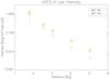 |
Fig. 10 UVCS H I Lyα line intensity at 1.77, 2.53, 3.03, 4.03, and 5.03 R⊙, along the streamer axis (85° PA, orange squares) and the southern boundary of the streamer (95° PA, green circles). The error bars are smaller than the symbol size for certain points. |
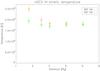 |
Fig. 11 UVCS H I kinetic temperature at 1.77, 2.53, 3.03, 4.03, and 5.03 R⊙, along the streamer axis (85° PA, orange diamonds) and the southern boundary of the streamer (95° PA, green triangles). |
Figures 5 and 11 show quite different electron and H I kinetic temperatures, particularly above 3.5–4.0 R⊙. Even if we consider the possibility of a broader instrumental profile, and then even lower values for the computed kinetic temperatures, the result is not consistent with the method used to determine the electron temperatures. Gibson et al. (1999) assumed a single fluid in the hydrostatic force balance, yielding an average temperature of the coronal gas rather than an actual electron or ion temperature. They justified their assumption by the results of Raymond et al. (1997), who found that electron and proton temperature were not significantly different in the core of their streamer, at heliocentric distances below 2 R⊙. At greater heights, where densities are much lower, this equality may not hold, and the results obtained by Gibson et al. (1999) are no longer reliable. In the attempt to remove this inconsistency, at least in part, we assumed a constant value of electron temperature when considering radial distances outside the streamer region. Figure 3 allows us to establish that measurements at heliocentric distances higher than 4.5 R⊙ at 85° PA (above the streamer cusp) and 3.5 R⊙ at 95° PA concern coronal regions out of the streamer. Therefore, above these heights, the electron temperature was assumed to be equal to Te = 8 × 105 cm-3 at 85° PA and Te = 7 × 105 cm-3 at 95° PA, as can be approximatively deduced from Fig. 5.
6. Solar wind outflow velocity profiles
To obtain the outflow velocity profiles in the equatorial streamer visible in March 2008 by theoretically reproducing the H I Lyα intensity measured by UVCS, we used the physical quantities previously described, substituting them into Eq. (1). We performed iterations on the wind velocity vw to reproduce the Lyα intensity measured by UVCS as closely as possible, and we restricted our analysis to the two radial paths at 85° and 95° PA. The values of H I outflow velocity were initially set equal to zero, which is reasonably supported by much observational evidence, suggesting that streamers are characterized by low-velocity outflows (e.g. Strachan et al. 2002; Uzzo et al. 2006).
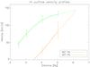 |
Fig. 12 Radial H I outflow velocity profiles along the streamer axis (85° PA, orange line) and the southern boundary of the streamer (95° PA, green line). The error bars refer to the uncertainties estimated at the various heliocentric distances as described in the text. |
Subsequently, the speeds were progressively increased to match the spectrometric observations, until obtaining the empirical velocity profiles reported in Fig. 12. The error bars were derived in terms of the lowest and highest speed values that still allow the observed line intensities to be reproduced, within the observational uncertainties (see Fig. 10). Along the streamer axis (85° PA), evidence of a significant deviation from static conditions only appears at about 3.5–4.0 R⊙, with an abrupt steepening of the outflow velocity profile at greater heliocentric distances. At latitudes corresponding to the southern boundary of the streamer (95° PA), the scenario is substantially different: the solar wind flows at velocities from 40 km s-1 at 2.5 R⊙ to 140 km s-1 at 5.0 R⊙.
In addition, by extrapolating the two curves of Fig. 12 up to 6.2 R⊙ (dashed lines), which is the maximum height where we calculated the electron density in the LASCO C2 FOV, the values of outflow speed appear to converge. Our results are higher by a factor of about 2 than those obtained by Spadaro et al. (2007) and Susino et al. (2008) within the streamer region, whereas the outflow velocities derived along the streamer boundary agree quite closely.
7. Discussion and conclusions
The present work is part of the studies dedicated to the observations of the coronal structures. We dealt with the data analysis of LASCO coronagraphic and UVCS spectrometric observations of an equatorial streamer at solar minimum. The results have allowed us to estimate the characteristics of a streamer, such as electron density, electron temperature, extent along the LOS, H I kinetic temperature, and outflow velocity. For the first time, we were able to directly derive all these physical properties from the observations, except for the H I outflow velocity, which was determined after theoretically reproducing the observed Lyα intensity.
In addition, we used the visible light images in total and polarized brightness to derive the intensity distribution of the F coronal component in the full FOV of LASCO C2. This technique can be adopted when B and pB are simultaneously known, and it avoids the use of an empirical expression for the F coronal emission, during investigation of the solar corona with visible-light coronagraphic observations. It is worthwhile noting that the fraction of polarization of the F-corona is negligible below 5 R⊙, and of the order of 1% at higher heliocentric distances. A good estimate of the stray light contribution is mandatory for getting meaningful results.
In the future, our results will contribute to defining the diagnostic techniques of the METIS coronagraph. The instrument is designed to make a unique contribution to the objectives of the Solar Orbiter mission; in particular, it will investigate the coronal region between 1.6 and 5.5 R⊙, which is crucial in linking the solar atmosphere phenomena to their evolution in the inner heliosphere. METIS will provide visible light and H I Lyα intensities of the coronal structures. However, since it was not conceived to provide line profiles from spectrometric observations, it will not allow the coronal H I velocity distribution to be estimated, which is a function of the proton kinetic temperature. This aspect induced us to investigate how the Lyα resonant scattering process depends on the kinetic temperature, under the condition of assuming its value.
Figure 13 reports four normalized scattering profiles. These are expressed by the last integral in Eq. (1), and their shape and shift in wavelength depend on the value of kinetic temperature and solar wind velocity, respectively. The normalized incident H I Lyα chromospheric profile (i.e. divided by its total intensity It) proposed by Auchère (2005) is also reported. We selected THI = 2.6 × 10⁶ K and THI = 1.6 × 10⁶ K, which are approximatively the highest and lowest values derived from the UVCS observations examined in this work (see Fig. 11), and calculated the integral of the scattering profile subtended by the incident one, i.e. the overlapping between the two profiles, in the range of outflow velocity between 0 and 200 km s-1. We found that the overlapping is greater for the lower kinetic temperature, in the case of wind velocity equal to zero. Conversely, the overlapping is greater for the higher kinetic temperature, when the solar wind flows with high speed. Figure 14 shows the variation of overlapping (normalized intensity) as a function of the outflow velocity, for the two investigated kinetic temperature values. The modulus of the difference between the two previous curves indicates that an uncertainty within the range of kinetic temperature values measured by UVCS can induce an error up to 10% on the determination of the theoretical Lyα intensity. This can influence, in turn, the estimate of the H I outflow velocity up to ±10−20 km s-1. We also deduced that the THI value mostly affects the Lyα scattering at low heliocentric distances in the streamer region, where the solar wind flows with low velocity.
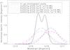 |
Fig. 13 Normalized incident H I Lyα chromospheric profile (black solid line) proposed by Auchère (2005) and four normalized scattering profiles depending on the value of kinetic temperature (THI = 2.6 × 10⁶ K, red lines, and THI = 1.6 × 10⁶ K, blue lines) and solar wind velocity (vw = 0 km s-1, dash-dot-dotted lines, and vw = 200 km s-1, long-dashed lines). |
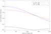 |
Fig. 14 Integral of the normalized scattering profile subtended by the incident chromospheric one in the outflow velocity range 0–200 km s-1 for THI = 2.6 × 10⁶ K (red line) and THI = 1.6 × 10⁶ K (blue line). The black line outlines the modulus of the difference between the two previous curves. |
We conclude that the knowledge of the kinetic temperature is fundamental to reliably evaluating the solar wind outflow velocity by using the Doppler dimming of the coronal H I Lyα line. In relation to the future investigations with METIS, it is necessary to compensate for the lack of spectrometric observations. A good opportunity is given by the UVCS Lyα observations carried out since 1996 until 2012. Such data can be used to determine a wide set of H I kinetic temperatures, which are relevant to different coronal structures and different phases of the solar activity cycle, in order to properly adopt them in the analysis of METIS observations. This extensive work will be the subject of a forthcoming investigation.
Available from the Harvard-Smithsonian Center for Astrophysics website: cfa-www.harvard.edu/uvcs
Acknowledgments
The authors thank the referee for helpful comments that led to a sounder version of the paper. The authors also thank A. Vourlidas for his help in computing the electron density by the inversion method of the visible light data. This work was partly supported by the Agenzia Spaziale Italiana through contract ASI/INAF No. I/013/12/0.
References
- Antonucci, E., Abbo, L., & Dodero, M. A. 2005, A&A, 435, 699 [NASA ADS] [CrossRef] [EDP Sciences] [Google Scholar]
- Antonucci, E., Fineschi, S., Naletto, G., et al. 2012, SPIE, 8443, 9 [Google Scholar]
- Auchère, F. 2005, ApJ, 622, 737 [NASA ADS] [CrossRef] [Google Scholar]
- Billings, D. E. 1966, A guide to the Solar Corona (New York: Academic Press) [Google Scholar]
- Brueckner, G. E., Howard, R. A., Koomen, M. J., et al. 1995, Sol. Phys., 162, 357 [NASA ADS] [CrossRef] [Google Scholar]
- Dolei, S., Bemporad, A., & Spadaro, D. 2014a, A&A, 562, A74 [NASA ADS] [CrossRef] [EDP Sciences] [Google Scholar]
- Dolei, S., Romano, P., Spadaro, D., & Ventura, R. 2014b, A&A, 567, A9 [NASA ADS] [CrossRef] [EDP Sciences] [Google Scholar]
- Domingo, V., Fleck, B., & Poland, A. I. 1995, Sol. Phys., 162, 1 [NASA ADS] [CrossRef] [Google Scholar]
- Fainshtein, V. G., Tsivileva, D. M., & Kashapova, L. K. 2010, Sol. Phys., 267, 203 [NASA ADS] [CrossRef] [Google Scholar]
- Fineschi, S., Gardner, L. D., Kohl, J. L., Romoli, M., & Noci, G. 1998, SPIE, 3443, 67 [Google Scholar]
- Frazin, R. A., Cranmer, S. R., & Kohl, J. L. 2003, ApJ, 597, 1145 [NASA ADS] [CrossRef] [Google Scholar]
- Gabriel, A. H. 1971, Sol. Phys., 21, 392 [NASA ADS] [CrossRef] [Google Scholar]
- Gibson, S. E., Fludra, A., Bagenal, F., et al. 1999, J. Geophys. Res., 104, 9691 [NASA ADS] [CrossRef] [Google Scholar]
- Hayes, A. P., Vourlidas, A., & Howard, R. A. 2001, ApJ, 548, 1081 [NASA ADS] [CrossRef] [Google Scholar]
- Hyder, C. L., & Lytes, B. W. 1970, Sol. Phys., 14, 147 [NASA ADS] [Google Scholar]
- Kaiser, M. L., Kucera, T. A., Davila, J. M., et al. 2008, Space Sci. Rev., 136, 5 [NASA ADS] [CrossRef] [Google Scholar]
- Kimura, H., & Mann, I. 1998, Earth Planets Space, 50, 493 [NASA ADS] [CrossRef] [Google Scholar]
- Kohl, J. L., Esser, R., Gardner, L. D., et al. 1995, Sol. Phys., 162, 313 [NASA ADS] [CrossRef] [Google Scholar]
- Kohl, J. L., Noci, G., Antonucci, E., et al. 1997, Sol. Phys., 175, 613 [NASA ADS] [CrossRef] [Google Scholar]
- Koutchmy, S., & Lamy, P. L. 1985, Properties and Interactions of Interplanetary Dust, eds. R. H. Giese, & P. L. Lamy (Dordrecht: Reidel), 63 [Google Scholar]
- Lemaire, P., Emerich, C., Vial, J.-C., et al. 2002, in From Solar Min to Max: Half a Solar Cycle with SOHO, ed. A. Wilson, ESA SP, 508 (Noordwijk: ESA), 219 [Google Scholar]
- MacQueen, R. M., Gosling, J. T., Hildner, E., et al. 1974, SPIE, 44, 207 [NASA ADS] [CrossRef] [Google Scholar]
- Mann, I. 1992, A&A, 261, 329 [NASA ADS] [Google Scholar]
- Minnaert, M. 1930, ZA, 1, 209 [Google Scholar]
- Müller, D., Marsden, R. G., St. Cyr, O. C., & Gilbert, H. R. 2013, Sol. Phys., 285, 25 [NASA ADS] [CrossRef] [Google Scholar]
- Noci, G., & Maccari, L. 1999, A&A, 341, 275 [NASA ADS] [Google Scholar]
- Noci, G., Kohl, J. L., & Withbroe, G. L. 1987, ApJ, 315, 706 [NASA ADS] [CrossRef] [Google Scholar]
- Priest, E. R. 1987, Solar Magneto-Hydrodynamics (Dordrecht: Reidel) [Google Scholar]
- Quémerais, E., & Lamy, P. 2002, A&A 393, 295 [NASA ADS] [CrossRef] [EDP Sciences] [Google Scholar]
- Raymond, J. C., Kohl, J. L., Noci, G., et al. 1997, Sol. Phys., 175, 645 [NASA ADS] [CrossRef] [Google Scholar]
- Saito, K., Poland, A. I., & Munro, R. H. 1977, Sol. Phys., 55, 121 [NASA ADS] [CrossRef] [Google Scholar]
- Spadaro, D., Susino, R., Ventura, R., Vourlidas, A., & Landi, E. 2007, A&A, 475, 707 [NASA ADS] [CrossRef] [EDP Sciences] [Google Scholar]
- Strachan, L., Suleiman, R., Panasyuk, A. V., Biesecker, D. A., & Kohl, J. L. 2002, ApJ, 571, 1008 [Google Scholar]
- Susino, R., Ventura, R., Spadaro, D., Vourlidas, A., & Landi, E. 2008, A&A, 488, 303 [NASA ADS] [CrossRef] [EDP Sciences] [Google Scholar]
- Uzzo, M., Strachan, L., Vourlidas, A., Ko, Y.-K., & Raymond, J. C. 2006, ApJ, 645, 720 [NASA ADS] [CrossRef] [Google Scholar]
- Van De Hulst, H. C. 1950, Bull. Astron. Inst. Netherland, 410, 135 [Google Scholar]
- Withbroe, G. L., Kohl, J. L., Weiser, H., & Munro, R. H. 1982, Space Sci. Rev., 33, 17 [NASA ADS] [CrossRef] [Google Scholar]
- Woods, T. N., Tobiska, W. K., Rottman, G. J., & Worden, J. R. 2000, J. Geophys. Res., 105, 27195 [NASA ADS] [CrossRef] [Google Scholar]
- Zangrilli, L., Nicolosi, P., Poletto, G., et al. 1999, A&A, 342, 592 [NASA ADS] [Google Scholar]
All Figures
|
Fig. 1 Adopted geometry for the resonant scattering process in the coronal point P. The Cartesian y-axis points outwards from the plane of the page. |
| In the text | |
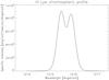 |
Fig. 2 Chromospheric H I Lyα line profile computed as a sum of 3 Gaussians (see Eq. (2)). |
| In the text | |
|
Fig. 3 LASCO C2 pB image taken at 9:00 UT on March 11, 2008, and UVCS slit positions at 1.77, 2.53, 3.03, 4.03, and 5.03 R⊙ above the east limb of the Sun. The dotted lines indicate the two radial paths along which we were able to determine the Lyα intensity from the UVCS observations. The dash-dotted line outlines the limb of the solar disk. |
| In the text | |
|
Fig. 4 Radial electron density profiles computed in the streamer region from 80° to 100° PA (dotted lines), while the solid line indicates, for comparison, the profile calculated by Gibson et al. (1999). The radial electron density profiles obtained at 85° PA (dashed line) and 95° PA (dash-dotted line) are shown. |
| In the text | |
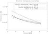 |
Fig. 5 As in Fig. 4, for the radial electron temperature profiles. |
| In the text | |
|
Fig. 6 Streamer extent at 85° PA as seen from the solar north pole. The black circle is the Sun, and the dash-dotted line indicates the border of the region hidden from the LASCO C2 occulter. The Cartesian X-axis of the heliocentric Earth equatorial (HEEQ) coordinate system points towards Earth, i.e. towards LASCO. |
| In the text | |
|
Fig. 7 Intensity map of the F-corona in the LASCO C2 FOV, obtained combining the total and polarized brightness taken on March 11, 2008, at 9:07 and 9:00 UT, respectively. The contour levels (dotted lines) are reported in units of 1 × 10⁻⁹ mean solar brightness (MSB). The solid line outlines the limb of the solar disk. |
| In the text | |
|
Fig. 8 Ellipticity of the F-corona intensity as given by Eq. (5). The plotted points refer to requatorial corresponding to the contour levels reported in Fig. 7. |
| In the text | |
|
Fig. 9 From left to right: coronal intensity at 90°, 270°, and 0° PA as a function of the heliocentric distance, in units of MSB. The solid line is the total brightness, the dashed line represents the K-corona emission, and the dotted line outlines the F-corona emission. The Koutchmy & Lamy (1985) F-corona model (dash-dotted line) is also reported for comparison. The total brightness was measured at 9:07 UT on March 11, 2008, and the K corona and F corona were derived by using the pB image taken at 9:00 UT on March 11, 2008. |
| In the text | |
|
Fig. 10 UVCS H I Lyα line intensity at 1.77, 2.53, 3.03, 4.03, and 5.03 R⊙, along the streamer axis (85° PA, orange squares) and the southern boundary of the streamer (95° PA, green circles). The error bars are smaller than the symbol size for certain points. |
| In the text | |
|
Fig. 11 UVCS H I kinetic temperature at 1.77, 2.53, 3.03, 4.03, and 5.03 R⊙, along the streamer axis (85° PA, orange diamonds) and the southern boundary of the streamer (95° PA, green triangles). |
| In the text | |
|
Fig. 12 Radial H I outflow velocity profiles along the streamer axis (85° PA, orange line) and the southern boundary of the streamer (95° PA, green line). The error bars refer to the uncertainties estimated at the various heliocentric distances as described in the text. |
| In the text | |
|
Fig. 13 Normalized incident H I Lyα chromospheric profile (black solid line) proposed by Auchère (2005) and four normalized scattering profiles depending on the value of kinetic temperature (THI = 2.6 × 10⁶ K, red lines, and THI = 1.6 × 10⁶ K, blue lines) and solar wind velocity (vw = 0 km s-1, dash-dot-dotted lines, and vw = 200 km s-1, long-dashed lines). |
| In the text | |
|
Fig. 14 Integral of the normalized scattering profile subtended by the incident chromospheric one in the outflow velocity range 0–200 km s-1 for THI = 2.6 × 10⁶ K (red line) and THI = 1.6 × 10⁶ K (blue line). The black line outlines the modulus of the difference between the two previous curves. |
| In the text | |
Current usage metrics show cumulative count of Article Views (full-text article views including HTML views, PDF and ePub downloads, according to the available data) and Abstracts Views on Vision4Press platform.
Data correspond to usage on the plateform after 2015. The current usage metrics is available 48-96 hours after online publication and is updated daily on week days.
Initial download of the metrics may take a while.