| Issue |
A&A
Volume 577, May 2015
|
|
|---|---|---|
| Article Number | A147 | |
| Number of page(s) | 10 | |
| Section | Planets and planetary systems | |
| DOI | https://doi.org/10.1051/0004-6361/201424620 | |
| Published online | 20 May 2015 | |
Characterizing spectral continuity in SDSS u′g′r′i′z′ asteroid photometry
1
Observatório Nacional (COAA), Rua General José Cristino 77, 20921-400
São Cristóvão, Rio de Janeiro RJ,
Brazil
e-mail:
This email address is being protected from spambots. You need JavaScript enabled to view it.
2
LESIA, Observatoire de Paris, CNRS, UPMC, Université
Paris-Diderot, 5 place Jules
Janssen, 92195
Meudon,
France
Received: 16 July 2014
Accepted: 7 March 2015
Abstract
Context. The 4th release of the SDSS Moving Object Catalog (SDSSMOC) is presently the largest photometric dataset of asteroids. Up to this point, the release of large asteroid datasets has always been followed by a redefinition of asteroid taxonomy. In the years that followed the release of the first SDSSMOC, several classification schemes using its data were proposed, all using the taxonomic classes from previous taxonomies. However, no successful attempt has been made to derive a new taxonomic system directly from the SDSS dataset.
Aims. The scope of the work is to propose a different interpretation scheme for gauging u′g′r′i′z′ asteroid observations based on the continuity of spectral features. The scheme is integrated into previous taxonomic labeling, but is not dependent on them.
Methods. We analyzed the behavior of asteroid sampling through principal components analysis to understand the role of uncertainties in the SDSSMOC. We identified that asteroids in this space follow two separate linear trends using reflectances in the visible, which is characteristic of their spectrophotometric features.
Results. Introducing taxonomic classes, we are able to interpret both trends as representative of featured and featureless spectra. The evolution within the trend is connected mainly to the band depth for featured asteroids and to the spectral slope for featureless ones. We defined a different taxonomic system that allowed us to only classify asteroids by two labels.
Conclusions. We have classified 69% of all SDSSMOC sample, which is a robustness higher than reached by previous SDSS classifications. Furthermore, as an example, we present the behavior of asteroid (5129) Groom, whose taxonomic labeling changes according to one of the trends owing to phase reddening. Now, such behavior can be characterized by the variation of one single parameter, its position in the trend.
Key words: catalogs / minor planets, asteroids: general / methods: statistical / astronomical databases: miscellaneous
© ESO, 2015
1. Introduction
Characterization of the compositional versus dynamical distribution of the asteroid population has relied on large datasets. In particular, the definition of asteroid classes, or taxonomies, has been historically linked to the development of new sets of asteroid observations. The first taxonomy, called CMZ (Chapman et al. 1975), began with the TRIAD catalog (Tucson Revised Index of Asteroid Data; Bowell et al. 1978). This dataset was composed of radiometric, photometric, and polarimetric measurements of 110 asteroids obtained from 1972 to 1978 (Morrison & Zellner 2007). The derived taxonomy divided the asteroids among S (“Stone”), C (“Carbonaceous”), and U (“Unclassified”), plus a single type representing Vesta alone.
The second generation of taxonomies, in the mid-1980s, was boosted by the Eight-Color Asteroid Survey (ECAS; Zellner et al. 1985) and gave birth to three taxonomic schemes: Tholen (1984), Barucci et al. (1987), and Tedesco et al. (1989). The so-called Tholen taxonomy (Tholen & Barucci 1989) used principal component analysis and minimal tree techniques to divide the asteroids into 14 classes – S, C, G, B, F, A, D, T, E, M, P, R and V – defined by their IRAS albedo and colors.
A third generation of taxonomies came with the advent of asteroid spectroscopy. Using visible spectra from the Small Main-belt Asteroid Spectroscopic Survey II (SMASS II) and a methodology similar to Tholens’ (plus visual inspection for spectral features), Bus & Binzel (2002) increased the number of classes to 26. Some years later, a near infrared (NIR) extension to this system, based on data for 371 asteroids (DeMeo & Binzel 2008), was developed by DeMeo et al. (2009), decreasing the number of classes to 23.
More recently, the release of the Sloan Digital Sky Survey (SDSS; Stoughton et al. 2002) and its subproduct, the Moving Objects Catalog (SDSSMOC; Ivezić et al. 2001, 2002), allowed the development of several studies analyzing the distribution and taxonomic classification of asteroids using the four colors of the survey. This is the largest asteroid color catalog available with about four hundred thousand detections and reaching asteroids as small as 1 km. Up to now, several authors have applied a myriad of different approaches in order to use its data to classify asteroids according to previous taxonomies (Ivezić et al. 2001; Nesvorný et al. 2005; Roig & Gil-Hutton 2006; Parker et al. 2008; Carvano et al. 2010). Even though these SDSS taxonomic classifications have proven to be extremely useful in characterizing the distribution of spectral types in the main belt, they also end up hiding much of the spectral diversity that may be present within each class (and between classes) in the SDSS dataset. Also, these methodologies are unable to detect any new spectral type that may exist in the sample.
An attempt to derive a new taxonomic system directly from the SDSS dataset was presented in a previous work (Hasselmann et al. 2013). In this paper, a modified version of the G-mode clustering algorithm was applied to the SDSSMOC. The G-mode algorithm is an unsupervised classification method that depends on only one free parameter, the confidence level q1. The final number of classes obtained varied with the adopted value of q1 from 1.0 to 3.0. However, subsequent tests showed that the classes obtained in this way were of limited practical use, since either the classes obtained were too inclusive in terms of spectral shapes or the number of unclassified samples ended up being too high.
The lack of success of this attempt is due to two characteristics of the SDSS dataset. One is the relatively high uncertainties of the observations of the fainter objects, which dominate the sample. The other is the sheer number of the observations in the dataset. Their combined effect is to blur the distinction between the classes.
Therefore, our goal here is to propose a different approach to interpreting u′g′r′i′z′ asteroid photometry. We investigate the continuity of spectral features and propose a more suitable scheme based on this assumption and only relying on the information given by the dataset. To interpret the proposed scheme, we then integrate it with the traditional taxonomies. We regard the present work mainly as exploratory, where the techniques used here are applicable to other datasets, such as the ones that will be generated by the Gaia mission (Delbó et al. 2012) and the LSSST (Jones et al. 2014).
A brief description of the SDSSMOC4 data and an explanation of the sampling procedure are given in Sects. 2 and 3. The technique for resolving and defining the identified trends are given in Sect. 3.3, while in Sect. 3.4 we add the Carvano groups to the new spatial configuration and discuss their placement in relation to the identified features and the scheme as a classification tool. The results are discussed in Sect. 4, along with the asteroid classification. We conclude and summarize our results in Sect. 5.
2. Selection of sample from SDSS Moving Object Catalog
The fourth release of SDSS Moving Objects Catalog is now the largest photometric dataset. of small solar system bodies (Ivezić et al. 2002; Ivezic et al. 2010), containing 471 569 detections of moving objects, where 202 101 are linked to 104 449 unique objects from the ASTORB list (Bowell et al. 1994). The SDSSMOC is composed of a sample of asteroids and, in much smaller number, comets (Solontoi et al. 2010). Moreover, the catalog may contain asteroid of sizes ranging from around 60 km (considering H = 11.0 and geometric albedo of 5%) to 700 m (H = 18.0 and geometric albedo of 25%) and members of several families (Parker et al. 2008).
Observations obtained from 519 observing runs up to March 2007, using the u′, g′, r′, i′z′ filter system (Fukugita et al. 1996) provide PSF magnitudes and the corresponding uncertainties at 355.7 nm, 482.5 nm, 626.1 nm, 767.2 nm, and 909.7 nm band centers and at bandwidths of 46.3 nm, 98.8 nm, 95.5 nm, 106.4 nm, and 124.8 nm, respectively. The PSF magnitude of the sources is measured by fitting the point spread function model to the detected objects (Stoughton et al. 2002). Since the colors were obtained almost simultaneously, rotational variations can be neglected for most of the observed asteroids. The SDSS magnitudes are in the asinh photometric system (Lupton et al. 1999), which are convert to flux density1 in order to derive the reflectances (Rj = { u,r,i,z }) corrected from solar contribution2 and normalized at g′ band.
In what follows, all observations of undesignated asteroids have been excluded, along with all detections 15 degrees from the Galactic plane owing to including sources in crowded stellar regions, and all observations with | Dec | < 1.26 and negative galactic latitude, as recommended by the SDSSMOC authors3. The resulting SDSSMOC sample contains 103 627 detections linked to 70 240 asteroids. In the following section, this sample was used to preliminarily characterize the spectral continuity and to select the best subsample for tracing their linear equation.
2.1. Analysis of the sample
All the major characteristics of asteroid spectra in the visible – presence of the 1 micron band, spectral slope, and drop in the UV – are sampled by the SDSS colors, and the relative importance of each characteristic is what ultimately defines the taxonomic classes (at least on the taxonomic schemes exclusively based on spectral information). These spectral characteristics induce correlations between the SDSS-derived reflectances.
Figure 1 shows the plots of Rr vs. Ri, Ri vs. Rz, and Ru vs. Rr for the selected SDSSMOC sample. In the first plot, a general positive correlation between the two variables is evident and reflects the behavior of the spectral slope of the asteroid spectra. In the second plot, the objects are more scattered, but some concentrations emerges overlapped with the general positive correlation between Ri and Rz, possibly implying a finer structure of the behavior of the sample in the reflectance space. Two denser clusters of objects are also present in the last plot, but Ru and Rr are not correlated.
To better understand the observed behaviors, we superimposed some taxonomic classes on these plots. To do so, we selected a sample composed of those SDSS asteroids that were previously observed spectroscopically and that have a reliable taxonomic classification. We chose the S3OS2 survey, a spectroscopic sample obtained with uniform instrumental conditions (Lazzaro et al. 2004), and we found 100 asteroids from this survey that have at least one SDSS detection. Using these “matching” observations, we calculated (1) the variance-covariance matrix of their four photometric variables and (2) the coordinates (and relative error bars) in the space of the photometric variables of the center of the taxonomic classes present in the sample. In Fig. 1, each taxonomic type is represented by an ellipse whose semi-axes are defined by the eigenvectors of the variance-covariance matrix (± 2σ) plotted over the SDSSMOC sample.
In the Ri and Rz plot, two different trends emerge when the taxonomic classes are taken into account: the first contains the taxonomic classes of asteroid with featureless spectra (B, C, X, and D types), which have a slightly higher slope than that of the whole sample; the other includes the taxonomic class to which asteroids presenting 1-micron absorption in their spectra belong (A, S and V types). However, the overlap of the taxonomic classes seen in Fig. 1 indicates that the reflectances are not the best variable space for quantifying trends in the spectral features. Another problem here is also the contamination of the dataset by noisy observations. In what follows, we transform the asteroid reflectance to the more suitable set of variables and derive a new methodology for obtaining the linear equation to observed trends.
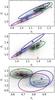 |
Fig. 1 SDSSMOC reflectances plotted beside the taxonomic locus of SDSS asteroids with S3OS2 classification. In the background, there is a density plot with all SDSS observations. |
3. Methodology
3.1. Principal component analysis
The issue of the best variable space can be addressed by applying principal component analysis (PCA), which has been widely used in connection with asteroid taxonomy and which constitutes the backbone of both Tholen and Bus taxonomic systems (Tholen 1984; Bus & Binzel 2002). PCA have also played an important role in the analysis of SDSS photometry before (Ivezić et al. 2002; Nesvorný et al. 2005; Roig & Gil-Hutton 2006).
The PCA rearranges all data placement and dimensionality by characterizing it through their principal correlated axes (e.g., Press et al. 1988; Jolliffe 1986). The principal components (abbreviated to PC for representing the variables and not the method) carry different amounts of sample variance, usually connected to information contained in data, allowing correlations in the data to become more pronounced. The PC were computed by singular value decomposition (Wall et al. 2003) method using the Scikit-learn package for the Python programming language (Pedregosa et al. 2011). We applied it with whitening and kept the same number of variables. The whitening is a normalization that rescales the data by dividing the component matrix by each PC standard deviations, thereby maximizing the output for real correlations and equalizing the variables. Whitening does not alter real correlations found in the data, but only improves visualization. Then, the equation of transformation of reflectances to PC is given by 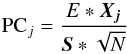 (1)where \begin{lxirformule}$\vec{X_{j}}$\end{lxirformule} is a SDSS observation, in reflectance; E is the eigenvector matrix, containing the weight of each reflectance on the definition of each PC in each row; S is the standard deviation vector; and N is the total sample size. The transformation gives us a new four-dimensional variable PCj.
We can now use the distribution of the principal components to visualize the relation between spectral characteristics and the SDSS reflectances better and to analyze how this is affected by uncertainties in the data.
3.2. Probing the role of the uncertainties in the SDSSMOC
Characteristics of the SDSSMOC samples.
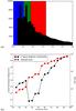 |
Fig. 2 a) Distribution of errors in the u′-band. The blue, green, and red backgrounds denote the Q1, Q2, and Q3, respectively. b) Plot of the u′-band normalized median error and sample size according to percentile ranks. |
The SDSSMOC contains observations of moving objects taken at different observational configurations, atmospheric conditions, stellar background, and position on the CCD. All these variables contribute to the uncertainties, or noise, of the data, which might reflect on the observed spectral continuity. Thus, to understand the effect of noise on the data set, the SDSSMOC sample was selected at three standard percentile ranks disstinguished in the distribution of uncertainties of the four filters. The percentile rank defines how much, in percentage points, of the data is found under an upper error limit. This kind of progressive sorting allows visualizing and analyzing the increase in the noise weight on the SDSSMOC sample.
We then used quartiles of the uncertainty distribution containing 25%, 50%, and 75% of the sample to define three subsamples: Q1, Q2, and Q3 (a given example in Fig. 2a presents the three sampling in the u′-band). Table 1 gives, for each SDSS filter, the upper error limits and sample size of Q1, Q2, and Q3, as well as their total standard deviation, total median uncertainties, and completeness. The completeness is the magnitude limit where the reliability of point sources to be detected drops to 95%, and the photometric measurements has lower quality4.
In Fig. 3, we plot PC3 vs. PC1 and PC3 vs. PC2 for the three quartiles, and it is clearly shown how the increase in the noise blurs the information contained in the data and the increase in size modifies the PC calculated independently for each sample. In PC3 vs. PC1 of Q1, the data distribution resembles what is observed by Warell & Lagerkvist (2007), which used 1332 SMASSII spectra to derive a taxonomic classification for Gaia photometric data. In our plot, two groups with elongated shapes appears. These two groups are related to spectra with and without absorption band (C and S). The remaining points are too sparse to derive any conclusion about their distribution. The PC3 vs. PC2, on the other hand, is dominated by the errors that blur the separation between the clusters of featureless spectra and spectra with the one-micron band.
In the PC space of Q2, it is possible to visualize two clear concentrations, spreading in the PC3 direction. These concentrations, which are better described as trends, are best resolved in the PC3 vs. PC2 space. It is noteworthy that although PC3 contains the largest spread, the largest part of the error is contained in PC1. Therefore, that these two concentrations are not unimodal outside the C and S groups indicates the existence of a continuous distribution of spectral types.
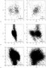 |
Fig. 3 PC2 vs. PC1 and PC3 vs. PC2 for a) 1st (Q1); b) 2nd (Q2); and c) 3rd quartile (Q3) samples. The principal components of each sample have been computed independently. The error bars, contained in the bottom right corner, represent the average uncertainty in the two axes. |
Finally, in Q3, the sample is highly dominated by uncertainties, and the C and S groups are barely distinguished from each other, although the trends are still visible. Moreover, there are no large differences between the eigenvector matrix of the Q2 and Q3, which indicates the robustness of these correlations in the data, which are unchanged even when the data quality decreases.
To select the sample that discerns the trends better, we then sampled the SDSSMOC uncertainties in several percentile ranks and computed the normalized median error for each SDSS filter. This quantity measures the relative importance of the formal photometric errors in the dispersion of the data. The result, when sampling from ranks of 15% to 100%, is that the normalized median error in Ru, Rr, Rz, and Ri vary from 25–82%, 7–18%, 10–15%, and 9–27%, respectively. The u′-band normalized median error has the largest variation, because this band has the lowest quantum efficiency among the four SDSS filters at five times less than the r′-band (Gunn et al. 1998). Nonetheless, we prefer not removing the u′-band, because it is the sole filter probing the near ultraviolet, and it brings important information, since in this spectral region, owing to charge transfer inside iron-bearing minerals, an absorption band may be present, causing a significant drop in the spectra.
Therefore, we decided to analyze the quality of each sample relative to the u′-band normalized median error. This behavior is shown in Fig. 2b, where three regimes of data sorting can be perceived. If the sampling is too restrictive, with scores below 30%, the sample size is too small and dominated by errors, as is the case for Q1 (Fig. 3a). If the sampling is loose, increase in sample size correlates to the increase in noise, which means that the sample is also dominated by errors. Therefore, only between scores of 30% to 50% do we find a minima in the u′ relative uncertainty and a near plateau in sample size. On the basis of these considerations, we decided to continue our analysis using Q2, since it offers the best ratio between uncertainty and size and keeps the trends clearly separated.
The eigenvector matrix (E) and W weight vector for SDSSMOC-Q2 are given by
![Mathematical equation: \begin{eqnarray} &&E=\left[\begin{array}{cccc} 0.228 & 0.296 & 0.289 & 0.286\\ -1.209 & 0.206 & 0.505 & 0.2378\\ 0.106 & 1.232 & 0.750 & -2.119\\ 1.075 & -4.762 & 4.973 & -0.955 \end{array}\right] \\[3mm] && \vec{W}=S^{2}/N=\left[\begin{array}{c} 0.82\\ 0.14\\ 0.04\\ 0.005 \end{array}\right] . \end{eqnarray}](/articles/aa/full_html/2015/05/aa24620-14/aa24620-14-eq26.png) Given vector W, then S can be easily derived. Vector W represents the variance weight ratio of each PC. The PC values of each SDSS observation can be computed by inserting E and S into Eq. (1). For Q2, N = 7190. The slope of the asteroid spectra is reflected in the large amount of variance contained in PC1, while PC4 can be neglected since it holds less than 1% of the total variance. The space PC2-PC3 will thus be used since it is the most representative.
Given vector W, then S can be easily derived. Vector W represents the variance weight ratio of each PC. The PC values of each SDSS observation can be computed by inserting E and S into Eq. (1). For Q2, N = 7190. The slope of the asteroid spectra is reflected in the large amount of variance contained in PC1, while PC4 can be neglected since it holds less than 1% of the total variance. The space PC2-PC3 will thus be used since it is the most representative.
The variables for the chosen subset are strongly linearily correlated as indicated by the 82% of variance accounted by PC1, which also contains an equal proportion of each SDSS band, implying that it is intrinsically connected to the spectral slope (Nesvorný et al. 2005). PC2 weighs on Ru and Ri, and the negative sign of the score of Ru means that when spectral slope is high, the ultraviolet drop is generally deeper. PC3 correlates with Rz, the variable containing the information on the one-micron silicate absorption band. Therefore, trends in the spectral features that are relevant to classification can now be discerned in PC space. To use this characteristic, we need to obtain equations of the axis that define the trends in the PC space.
3.3. The linear equations for the spectral trends in PC space
The next step in our analysis will be to obtain the linear equations for the trends that can be used for classification and quantification purposes. To perform this, we divided the observations into regions and replaced them by vector, where the only information kept was their position and their direction. Then, we clustered them according to their vicinity and common alignment. This was performed by applying a multidimensional histogram tool from Numpy5 and Scipy.hierarchy tools6. The procedure is summarized in the following steps:
-
1.
The SDSSMOC-Q2 is partitioned into four-dimensional cells,were each PC is divided into seven regions (74 = 2401 cells).
-
2.
Cells containing over 15 observations had their PC median (xi) and variance-covariance matrix recorded. The median gives the center of the cells, while the first eigenvector (ei) of variance-covariance matrix indicates the main direction of correlation of each cell.
-
3.
The distance among all cells are calculated through the equation:
 The first eigenvector is included in the distance equation to account for cells of similar orientation.
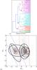
Fig. 4 a) Binary tree dendrogram. Each superior node supports several lower pairs. Different colors highlight the biggest nodes. b) Trends. The ellipses are the representation in PC space of the nodes of same roman letter in panel a). The nodes I and IV represent the equation for the Blue and Red trends. The contours are the projected ellipsoids. The dotted lines are the projected cylinder obtained through the secondary eigenvectors of the variance-covariance matrix of the I and IV nodes.
-
4.
The cells are hierarchically arranged according to their distances as computed above. Similar cells are organized by pairs until reaching a binary tree structure (Bentley 1979). The dendrogram in Fig. 4a shows how the sectors are coordinated. The nodes are points where pairs met, representing the pairs below and forming a supercluster. Inspecting the nodes allowed us to search for correlation features among the observations, such as the observed trends.
-
5.
Two nodes (I and IV, Fig. 4b) contain most of the samples belonging to the trends recognized in the previous analysis. These nodes form superclusters that have the median and variance-covariance matrix calculated from all observations composing it. From the variance-covariance matrices, we computed the four eigenvectors that gives four main axes of each supercluster. The first eigenvector is the main axis, and it represents the orientation and direction of the trends. Then, from the main axis we obtain the linear equation for each trend in the full PC space:


From now on, we decided to address the one-micron band featured and featureless trends to Red and Blue, because of the colors chosen to represent them in Fig. 4b.
These equations allow us to compute the observation’s distance (d) from and position (z) for each trend. The projection of the lines describing the two trends on the PC3-PC2 plane are given in Fig. 4b. The position in the main axis of one trend quantifies the intensity of the related spectral feature (band depth or spectral slope/UV-drop) and is calculated by the scalar product of the main axis vector and the observation vector PCj. An observation is regarded as belonging to one trend if its distance with respect to each trend center satisfies the following condition: ![Mathematical equation: \begin{eqnarray} \vec{d}_{\rm red}&=&\left[\begin{array}{cccc} -0.1195 & -0.5328 & -0.0056 & -0.8377\\ -0.0944 & -0.8325 & -0.0518 & 0.5434\\ 0.9854 & -0.1472 & 0.0716 & -0.0474 \end{array}\right] \nonumber \\[2mm] && \times \left[\begin{array}{c} PC1-0.204\\ PC2-0.590\\ PC3+0.154\\ PC4-0.694 \end{array}\right]_{\rm obs} \\[2mm] \vec{d}_{\rm blue}&=&\left[\begin{array}{cccc} -0.2306 & 0.2464 & -0.0755 & -0.9382\\ 0.0324 & 0.8577 & 0.4810 & 0.1786\\ 0.9263 & -0.1086 & 0.2335 & -0.2750 \end{array}\right]\nonumber \\[2mm] && \times \left[\begin{array}{c} PC1+0.147\\ PC2+1.201\\ PC3+0.407\\ PC4-0.788 \end{array}\right]_{\rm obs} \end{eqnarray}](/articles/aa/full_html/2015/05/aa24620-14/aa24620-14-eq40.png)
 where the three rows of the matrix are given by the secondary eigenvectors characterizing each trend. It is important to note that one observation may belong to a single trend or to both.
3.4. Locus of asteroid classes
Once the trends are defined in the PC2-PC3 plane, we can relate them to the asteroid taxonomic classification and look where the groups are located in this PC space. The superposition of the taxonomic classes to the PC2-PC3 plot will help in interpreting the meaning of the two trends in terms of the spectral behavior of the asteroid. We decided to use the photometric classification available in the literature (Hasselmann et al. 2011) to which we add the B group (not included in the original work) using SDSSMOC observations spectroscopically classified as B and F in Neese (2010). We applied the same procedure as described in Sect. 3 to insert these taxonomic groups in the PC space. Figure 5 shows the 2σ locus of each class overlapped with the distribution of Q2.
The center of the classes in the PC space can now be projected into both axes defining the trends. For each class in each trend, Table 2 gives its distance and position, as defined in Sect. 3.3. The values of the z-distances along each trend were shifted so that the S class is at the origin of the Red trend and the C class is at the origin of the Blue trend. The position of the class in each trend and their possible interpretations are discussed further in the following section.
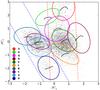 |
Fig. 5 Loci of the taxonomic classes in PC3 vs. PC2 space, represented by ellipses where the axes represent 2σ of the distributions. The 2σ confidence region for the Blue and the Red trends is indicated by the dotted lines. |
Distance and position of the center of the taxonomic groups on the trends.
4. Discussion
In the scheme represented by Fig. 5, the Blue contains the asteroid belonging to the C→X→D classes characterized by featureless spectra, while the Red trend refers to asteroid classified as L→S→Q→V types that have absorption features in their spectra. As expected, C and S classes gather most of observations for each trend, while all the other classes seem to “leak” out from them. Following the B→D direction in the Blue trend, the spectral slope increases as a consequence of the PC2 along the trend, corresponding to a deeper and deeper drop in the u′-band reflectance. The Red trend vertically crosses the PC2-PC3 plane at quasi constant values of PC2 in the direction L→V. There is clearly a spectral continuity from spectra with a higher slope bearing hints of a 1-micron shallow band to spectra with lower slopes and deeper bands. The O and A loci fall partially out of the confidence region of the Red trend and, together with the Q-types locus, form a O→Q→A sequence, almost parallel to the Blue trend. This sequence has its change in spectral slope and u′-band drop. They have similar evolution to the Blue trend, where both features increase from O→A, so much like the C→D sense.
It is noteworthy that there are diverse loci that are largely superimposed, in particular, C and X, S and L, and S and Q. Such superimposition is observed in all the PC space and is not an effect of projection. These classes have differences that are based solely on the varied strength of their spectral features, mostly spectral slope and depth of silicate band, which we have demonstrated are continuous.
This is therefore a direct consequence of the adopted reference taxonomy and the lack of some of these criteria when a different set of variables is used. In our representation what is important is that spectrophotometric data have an internal coherence, that is to say that a continuum of the spectral behavior of the asteroids of the SDSSMOC is maintained. In fact the aim of our analysis is to discuss and interpret the structure of that continuum and to use it to better characterize the analyzed population, as well as to gauge observational effects (i.e., phase reddening), which may modify the specta of asteroids. This kind of approach has been done on much smaller data sets by Bell (1986) and by Barucci et al. (1987).
Bell collapsed the Tholen taxonomic classes into three superclasses (primitive, igneous, metamorphic), thereby accounting for the degree of metamorphic heating the asteroid has undergone. Barucci et al. propose four evolutionary trends to interpret the asteroid composition nature through a taxonomy scheme based on the ECAS (Zellner et al. 1985) and the IRAS albedo catalog. These trends account for i) the volatile content reduction; ii) the evolution of the primitive solar nebula condensate toward enstatite silicates; iii) the increasing of the differentiation; and iv) the effect of the collision and fragmentation of differentiated bodies. Since that work, however, it has been realized that there are several factors that may influence the shape of an asteroid spectrum that is not directly related to composition. Two examples are space weathering (Moroz et al. 1996; Gaffey 2010; Lantz et al. 2013; Miller et al. 2014) and phase reddening (Sanchez et al. 2012).
The Blue trend accounts for the dark primitive asteroids. Increasing values of PC3 could be interpreted in terms of variation in the bulk chemical and mineralogical composition from the more primitive (D type) toward the more evolved dark B-type objects (Yang & Jewitt 2010; Perna et al. 2014), which could also account for a decrease in volatiles or organics present on their surfaces. However, similar effects could also arise from space weathering or phase reddening. Also, spectra of asteroids with compositions similar to enstatite chondrites and achondrites and metallic meteorites would also fall in this blue trend (i.e., Carvano et al. 2003). Finally, asteroids with compositions dominated by olivine-pyroxene whose bands have been suppressed for any reason (i.e., Reddy et al. 2011, 2014) would also plot on the Blue trend.
The Red trend describes the behavior of the spectra of asteroids dominated by a olivine-pyroxene composition. Increasing values of PC3 could indicate their difference in the silicate compositions that are characterized by a progressive increase in the amount of pyroxene-olivine going from L to V types. Nonetheless, phase reddening and space weathering also affect the PC3 by changing the spectral slope and band depth, which moves the asteroid spectrum in the trend’s direction. Inside the confidence band of both trends, not much can be said about variability on the PC2, where the errors have a major influence. Objects having more extreme spectral characteristics (such as those of A or O asteroids) occupy the border of the trend’s band of confidence.
4.1. Asteroid classification
One application of the methodology developed in the previous section is to classify the spectra of asteroids according to their position inside the trends. To this effect we gathered the complete SDSSMOC sample of 202 101 detections and classified using the procedure described in Sect. 3.3. We obtain a classification of 139 233 observations corresponding to 79 647 asteroids, where 39.85% belongs to Blue/featureless trend and 54.05% to the Red/featured trend. Only 5.85% of the observations are contained in the region intersected by both trends. Although carrying less information about the shape of spectra when compared to other proposed classification schemes, this classification can be applied to a considerably larger number of observations. In comparison with the previous SDSSMOC classification by Carvano et al. (2010), we find an increase of 29.5% in the capability of classifying asteroid observations, which could not be classified by the authors. This represents 31 767 new observations being classified.
 |
Fig. 6 a) Eight SDSS observations of asteroid (5129) Groom plotted in the scheme proposed. The error bars represent the errors transformed to PC space. The spectra of the observations are plotted together in the lower corner of the graph. The specific SDSS observation IDs are s14307, s0e2e7, sca267, sc8e1d, scf0dc, scdde4, scc719, and scbc65. b) Three asteroids with multiple observations presenting spectral variability. The SDSSMOC observation IDs for each asteroid: (2252) CERGA (blue): s3bafc, s3f6f3, s3eea4, s41189, s424bf, sbbb68, sf0125, sef985, sef5d2; (3631) Sigyn (purple): s16290, s16001, sf0e38, s042fc, s132c2; and (55926) 1998 FE60 (black): s17150, s18825, s17c18, s3924d, s2cd9b. |
A second application of the developed methodology is to provide an alternative way to classify asteroids on SDSS-based taxonomies. This can be accomplished by calculating the PC using Eqs. (1)–(3) and then plotting the coordinates in a diagram like Fig. 5, along with the boundaries of each class. Besides this visual classification is also possible to calculate the distance to the center of the taxonomic groups. These distances are also a quantitative indicator of how much the spectra of the observation deviates from each class template, which corresponds to the center each group. This allows for more efficient automated searches for specific spectral characteristics.
As example of one application of our scheme, we selected one asteroid, (5129) Groom, observed eight times by the SDSS. In Hasselmann et al. (2011), (5129) Groom is classified as Sp, but one observation is Lp, and the other one is Sp/Lp. When we plot these observations in Fig. 6a, we find them contained inside the Red trend, although spanning three groups: L, S, and Q. Using the scheme proposed here, we are thus able to verify that the observations increase in their zred from − 0.571, so well inside the L group, up to 0.591, at the bottom of the Q group. This variability cannot be attributed to phase reddening, owing to the small phase angle range (from 4.5 up to 11 degrees) of the diverse observations, and might be related to compositional differences across the object surface.
We may extend this application and verify asteroid spectral variabilities inside the boundaries of the taxonomic groups. We present in Fig. 6b, for example, three asteroids with multiple observations in the B group: (2252) CERGA (9 obs.), (3631) Sigyn (5 obs.), and (55926) 1998 FE60 (5 obs.). All these asteroids present spectral variablity that exceeds their intrinsical errors and the average uncertainty of all SDSSMOC-Q2 sample. The variability is substantial not only along the PC3, but also along the PC2, as in the case of the asteroid (2252) CERGA.
5. Conclusions and results
Using a subset of the visible reflectances from the SDSSMOC catalog, we found that asteroids follow mainly two continuous trends that describe their spectral behavior. These are barely visible in the reflectance space, but emerge clearly when data are translated into the PC space. Information drawn from the adopted dataset is contained within a band of the PC2-PC3 plane defined by the direction of each trend. These trends represent the evolutionary track of the two main characteristics of asteroid spectra: the presence and depth of the 1-μm band and the spectral slope.
It is noteworthy that most of the classified SDSSMOC data belongs to one of the two trends. A total of 29.5% more of the objects have been classified in Carvano et al. (2010). This demonstrates that some objects in between the formal taxonomic classes are taken into account. The given equations for the lines representing the trends, allows any object to be classified (asteroid, meteorite, or comet) for which the u′g′r′i′z′ photometry is available.
As a data product resulting from this work, we applied the PC transformation given in Eq. (1) to all observations of the SDSSMOC, and then used Eqs. (4) and (5) to calculate the distances of each observations along the axis that describe each trend. These lists will be made available as a product in the NASA PDS Archive, along with a revised version of the classification by Carvano et al. (2010), which includes the B class. The classification can be used to perceive how any observation compares with the template spectra of a given class in terms of band depth and spectral slope, allowing more refined searches inside the large data sets as the SDSSMOC. For this purpose, all SDSSMOC observations were further classified as Red, Blue or Red+Blue. In this sense, the scheme here described, although carrying less information, is more appropriate for observations outside the formal taxonomic boundaries.
In conclusion, we were able to distinguish the basic asteroid spectra trends by analyzing a selected sample of high-quality observations from SDSSMOC data. The addition of taxonomic locus helped us to give a compositional interpretation to both trends. Although the scheme was derived from a specific dataset, any observation in a similar photometric system, or any low-resolution spectrum convoluted with SDSS bandpasses, may also be classified.
http://www.sdss3.org/dr8/imaging/other_info.php#completeness
Acknowledgments
The authors thank CNPq, process No. 402085/2012-4, for the support. FAPERJ and CAPES are also acknowledged for diverse grants and fellowships to D.L., J.M.C., and P.H.H.
References
- Barucci, M. A., Capria, M. T., Coradini, A., & Fulchignoni, M. 1987, Icarus, 72, 304 [NASA ADS] [CrossRef] [Google Scholar]
- Bell, J. F. 1986, in Lunar and Planetary Sci. Conf., 17, 986 [Google Scholar]
- Bentley, J. L. 1979, IEEE Trans. Software Eng., 5, 333 [CrossRef] [Google Scholar]
- Bowell, E., Chapman, C. R., Gradie, J. C., Morrison, D., & Zellner, B. 1978, Icarus, 35, 313 [NASA ADS] [CrossRef] [Google Scholar]
- Bowell, E., Muinonen, K., & Wasserman, L. H. 1994, in Asteroids, Comets, Meteors 1993, eds. A. Milani, M. di Martino, & A. Cellino, IAU Symp., 160, 477 [Google Scholar]
- Bus, S. J., & Binzel, R. P. 2002, Icarus, 158, 146 [NASA ADS] [CrossRef] [Google Scholar]
- Carvano, J. M., Mothé-Diniz, T., & Lazzaro, D. 2003, Icarus, 161, 356 [NASA ADS] [CrossRef] [Google Scholar]
- Carvano, J. M., Hasselmann, P. H., Lazzaro, D., & Mothé-Diniz, T. 2010, A&A, 510, A43 [NASA ADS] [CrossRef] [EDP Sciences] [Google Scholar]
- Chapman, C. R., Morrison, D., & Zellner, B. 1975, Icarus, 25, 104 [NASA ADS] [CrossRef] [Google Scholar]
- Delbó, M., Gayon-Markt, J., Busso, G., et al. 2012, Planet. Space Sci., 73, 86 [NASA ADS] [CrossRef] [Google Scholar]
- DeMeo, F., & Binzel, R. P. 2008, Icarus, 194, 436 [NASA ADS] [CrossRef] [Google Scholar]
- DeMeo, F. E., Binzel, R. P., Slivan, S. M., & Bus, S. J. 2009, Icarus, 202, 160 [NASA ADS] [CrossRef] [Google Scholar]
- Fukugita, M., Ichikawa, T., Gunn, J. E., et al. 1996, ApJ, 111, 1748 [Google Scholar]
- Gaffey, M. J. 2010, Icarus, 209, 564 [NASA ADS] [CrossRef] [Google Scholar]
- Gunn, J. E., Carr, M., Rockosi, C., et al. 1998, AJ, 116, 3040 [NASA ADS] [CrossRef] [Google Scholar]
- Hasselmann, P. H., Carvano, J. M., & Lazzaro, D. 2011, NASA Planetary Data System, 145 [Google Scholar]
- Hasselmann, P. H., Carvano, J. M., & Lazzaro, D. 2013, in Proc. 12th Python in Science Conf. (SciPy 2013), 48 [Google Scholar]
- Ivezić, Ž., Tabachnik, S., Rafikov, R., et al. 2001, ApJ, 122, 2749 [Google Scholar]
- Ivezić, Z., Juric, M., Lupton, R. H., Tabachnik, S., & Quinn, T. 2002, in SPIE Conf. Ser. 4836, eds. J. A. Tyson, & S. Wolff, 98 [Google Scholar]
- Ivezic, Z., Juric, M., Lupton, R. H., et al. 2010, NASA Planetary Data System, 124 [Google Scholar]
- Jolliffe, I. T. 1986, Principal Component Analysis (New York: Springer-Verlag) [Google Scholar]
- Jones, R. L., Ivezic, Z., Malhotra, R., et al. 2014, in AAS/Division for Planetary Sciences Meeting Abstracts, 46, 214.13 [Google Scholar]
- Lantz, C., Clark, B. E., Barucci, M. A., & Lauretta, D. S. 2013, A&A, 554, A138 [NASA ADS] [CrossRef] [EDP Sciences] [Google Scholar]
- Lazzaro, D., Angeli, C. A., Carvano, J. M., et al. 2004, Icarus, 172, 179 [CrossRef] [Google Scholar]
- Lupton, R. H., Gunn, J. E., & Szalay, A. S. 1999, ApJ, 118, 1406 [Google Scholar]
- Miller, K. A., De Ruette, N., Harlow, G., Domingue, D. L., & Savin, D. W. 2014, in AAS Meet. Abstr., 224, 119.11 [Google Scholar]
- Moroz, L. V., Fisenko, A. V., Semjonova, L. F., Pieters, C. M., & Korotaeva, N. N. 1996, Icarus, 122, 366 [NASA ADS] [CrossRef] [Google Scholar]
- Morrison, D., & Zellner, B. 2007, NASA Planetary Data System, 74 [Google Scholar]
- Neese, C. 2010, NASA Planetary Data System, 123 [Google Scholar]
- Nesvorný, D., Jedicke, R., Whiteley, R. J., & Ivezić., Ž. 2005, Icarus, 173, 132 [NASA ADS] [CrossRef] [Google Scholar]
- Parker, A., Ivezić, Ž., Jurić, M., et al. 2008, Icarus, 198, 138 [NASA ADS] [CrossRef] [Google Scholar]
- Pedregosa, F., Varoquaux, G., Gramfort, A., et al. 2011, J. Machine Learning Res., 12, 2825 [Google Scholar]
- Perna, D., Alvarez-Candal, A., Fornasier, S., et al. 2014, A&A, 568, L6 [NASA ADS] [CrossRef] [EDP Sciences] [Google Scholar]
- Press, W. H., Flannery, B. P., Teukolsky, S. A., & Vetterling, W. T. 1988, Numerical Recipes in C: The Art of Scientific Computing (New York: Cambridge University Press) [Google Scholar]
- Reddy, V., Carvano, J. M., Lazzaro, D., et al. 2011, Icarus, 216, 184 [NASA ADS] [CrossRef] [Google Scholar]
- Reddy, V., Sanchez, J. A., Bottke, W. F., et al. 2014, Icarus, 237, 116 [NASA ADS] [CrossRef] [Google Scholar]
- Roig, F., & Gil-Hutton, R. 2006, Icarus, 183, 411 [NASA ADS] [CrossRef] [Google Scholar]
- Sanchez, J. A., Reddy, V., Nathues, A., et al. 2012, Icarus, 220, 36 [NASA ADS] [CrossRef] [Google Scholar]
- Solontoi, M., Ivezić, Ž., West, A. A., et al. 2010, Icarus, 205, 605 [NASA ADS] [CrossRef] [Google Scholar]
- Stoughton, C., Lupton, R. H., Bernardi, M., et al. 2002, ApJ, 123, 485 [Google Scholar]
- Tedesco, E. F., Williams, J. G., Matson, D. L., et al. 1989, ApJ, 97, 580 [Google Scholar]
- Tholen, D. J. 1984, Ph.D. Thesis, Arizona Univ., Tucson [Google Scholar]
- Tholen, D. J., & Barucci, M. A. 1989, in Asteroids II, eds. R. P. Binzel, T. Gehrels, & M. S. Matthews, 298 [Google Scholar]
- Wall, M. E., Rechtsteiner, A., & Rocha, L. M. 2003, in A Practical Approach to Microarray Data Analysis, eds. Berrar D. P., Dubitzky W., & Granzow M. (Norwel: Kluwer), 91 [Google Scholar]
- Warell, J., & Lagerkvist, C.-I. 2007, A&A, 467, 749 [NASA ADS] [CrossRef] [EDP Sciences] [Google Scholar]
- Yang, B., & Jewitt, D. 2010, AJ, 140, 692 [NASA ADS] [CrossRef] [Google Scholar]
- Zellner, B., Tholen, D. J., & Tedesco, E. F. 1985, Icarus, 61, 355 [NASA ADS] [CrossRef] [Google Scholar]
All Tables
All Figures
|
Fig. 1 SDSSMOC reflectances plotted beside the taxonomic locus of SDSS asteroids with S3OS2 classification. In the background, there is a density plot with all SDSS observations. |
| In the text | |
|
Fig. 2 a) Distribution of errors in the u′-band. The blue, green, and red backgrounds denote the Q1, Q2, and Q3, respectively. b) Plot of the u′-band normalized median error and sample size according to percentile ranks. |
| In the text | |
|
Fig. 3 PC2 vs. PC1 and PC3 vs. PC2 for a) 1st (Q1); b) 2nd (Q2); and c) 3rd quartile (Q3) samples. The principal components of each sample have been computed independently. The error bars, contained in the bottom right corner, represent the average uncertainty in the two axes. |
| In the text | |
|
Fig. 4 a) Binary tree dendrogram. Each superior node supports several lower pairs. Different colors highlight the biggest nodes. b) Trends. The ellipses are the representation in PC space of the nodes of same roman letter in panel a). The nodes I and IV represent the equation for the Blue and Red trends. The contours are the projected ellipsoids. The dotted lines are the projected cylinder obtained through the secondary eigenvectors of the variance-covariance matrix of the I and IV nodes. |
| In the text | |
|
Fig. 5 Loci of the taxonomic classes in PC3 vs. PC2 space, represented by ellipses where the axes represent 2σ of the distributions. The 2σ confidence region for the Blue and the Red trends is indicated by the dotted lines. |
| In the text | |
|
Fig. 6 a) Eight SDSS observations of asteroid (5129) Groom plotted in the scheme proposed. The error bars represent the errors transformed to PC space. The spectra of the observations are plotted together in the lower corner of the graph. The specific SDSS observation IDs are s14307, s0e2e7, sca267, sc8e1d, scf0dc, scdde4, scc719, and scbc65. b) Three asteroids with multiple observations presenting spectral variability. The SDSSMOC observation IDs for each asteroid: (2252) CERGA (blue): s3bafc, s3f6f3, s3eea4, s41189, s424bf, sbbb68, sf0125, sef985, sef5d2; (3631) Sigyn (purple): s16290, s16001, sf0e38, s042fc, s132c2; and (55926) 1998 FE60 (black): s17150, s18825, s17c18, s3924d, s2cd9b. |
| In the text | |
Current usage metrics show cumulative count of Article Views (full-text article views including HTML views, PDF and ePub downloads, according to the available data) and Abstracts Views on Vision4Press platform.
Data correspond to usage on the plateform after 2015. The current usage metrics is available 48-96 hours after online publication and is updated daily on week days.
Initial download of the metrics may take a while.