| Issue |
A&A
Volume 576, April 2015
|
|
|---|---|---|
| Article Number | L1 | |
| Number of page(s) | 4 | |
| Section | Letters | |
| DOI | https://doi.org/10.1051/0004-6361/201525650 | |
| Published online | 13 March 2015 | |
Molecular clouds have power-law probability distribution functions
1 University of Milan, Department of Physics, via Celoria 16, 20133 Milan, Italy
e-mail: This email address is being protected from spambots. You need JavaScript enabled to view it.
2 University of Vienna, Türkenschanzstrasse 17, 1180 Vienna, Austria
3 Harvard-Smithsonian Center for Astrophysics, Mail Stop 72, 60 Garden Street, Cambridge, MA 02138, USA
Received: 12 January 2015
Accepted: 9 February 2015
Abstract
In this Letter we investigate the shape of the probability distribution of column densities (PDF) in molecular clouds. Through the use of low-noise, extinction-calibrated Herschel/Planck emission data for eight molecular clouds, we demonstrate that, contrary to common belief, the PDFs of molecular clouds are not described well by log-normal functions, but are instead power laws with exponents close to two and with breaks between AK ≃ 0.1 and 0.2 mag, so close to the CO self-shielding limit and not far from the transition between molecular and atomic gas. Additionally, we argue that the intrinsic functional form of the PDF cannot be securely determined below AK ≃ 0.1 mag, limiting our ability to investigate more complex models for the shape of the cloud PDF.
Key words: ISM: clouds / dust, extinction / ISM: structure / methods: data analysis
© ESO, 2015
1. Introduction
In the past couple of decades, the column density probability distribution function of dark molecular clouds (hereafter PDF) has received much attention. The PDF is arguably one of the easiest quantities to measure (but see below Sect. 2). Moreover, it is robustly predicted by many theoretical studies (e.g. Vazquez-Semadeni 1994; Padoan et al. 1997; Scalo et al. 1998; Federrath et al. 2010) to follow a log-normal distribution, and this prediction has been apparently confirmed (at least up to a few magnitudes of visual extinction) by several observations (Lombardi et al. 2008; Goodman et al. 2009; Lombardi et al. 2010, 2011; Schneider et al. 2013; Alves de Oliveira et al. 2014; but see Tassis et al. 2010). Finally, departures from log-normality at high densities have been associated to the star formation activity of molecular clouds (e.g., Kainulainen et al. 2009; Lombardi et al. 2010; Schneider et al. 2013; see also Kainulainen et al. 2014).
In spite of the profuse efforts to measure the PDF, many of the observational results obtained so far are lacking a rigorous discussion of their range of validity and of the possible systematic effects on them. Moreover, PDFs obtained from various observations have been compared to the theoretical log-normal model, ignoring the limitations of both the observations and the theoretical predictions.
In this Letter we reconsider the measurements of PDFs and show that many of the claims made so far do not pass critical scrutiny. We highlight a number of observational issues related to the measurements of the PDF and show that this quantity cannot be robustly measured below AK ~ 0.1 mag. Using dust emission maps obtained from Herschel and Planck data, we show that for AK ≳ 0.2 mag, the PDFs of different molecular clouds follow with good approximation a power law, whose slope in many cases appears to be close to, or slightly steeper than, −2. Finally, in the range 0.1 mag, to 0.2 mag, there is a break from the power law at low extinctions.
2. Limitations in the measurement of the PDF
Technically, the PDF is derived as a simple (normalized) histogram of the column density measurements within some area of the sky that includes a molecular cloud. We assume here that the column density measurements are expressed in terms of K-band extinction AK and that data are binned in log 10AK (that is, the PDF is really a probability distribution for the logarithm base ten of the extinction). A direct bin in AK is also possible, and the associated probability distribution differs from the logarithmic one by a simple multiplicative term ∝AK.
Molecular clouds are mostly made of molecular hydrogen and helium, two species which are very difficult to detect at the low temperatures that characterize these objects. As a result, the column density of molecular clouds, from which the PDF is derived, is generally obtained from different tracers, such as dust (extinction in the optical and near-infrared and thermal emission in the far-infrared and submillimeter) or molecules with significant dipole moments (such as  CO or
CO or  CO). Each method has different advantages and limitations that should be understood and taken into consideration when comparing the observational PDFs with the theoretical predictions.
In the rest of this Letter, we assume that column density measurements are obtained through unbiased estimators. In reality, different techniques suffer from various biases, which will affect different parts of the PDF. However, a discussion of the biases related to column density measurements is beyond the scope of this Letter. Here, instead, we consider biases arising in the PDFs from unbiased column density measurements. Specifically, here we minimize measurement biases by using a combination of Herschel and Planck/IRAS emission data, calibrated with a 2MASS/Nicest extinction map (following Lombardi et al. 2014).
In general, PDFs are affected by four main biases: resolution, noise, boundaries, and superposition effects, which are the subjects of the following sections.
2.1. Resolution and noise biases
Each method of probing the column density has a finite resolution and different noise levels (with the two being inversely proportional to each other, for a given sensitivity). The effects of a finite resolution on the PDF are difficult to predict and quantify, because they depend on the (unresolved) small-scale structure of the cloud. Generally, extinction measurements demonstrate that clouds tend to be relatively smooth at low column densities; i.e., they show only small local variations in extinction, compared to their denser parts, which are very uneven, and therefore the most affected by resolution (see Lombardi et al. 2010). Thus, observations with finite resolutions will often “move” mass from the denser parts to the less dense ones, and the observed PDFs will thus show a lack of dense material.
The effects of statistical noise can instead be characterized better: noise acts by smoothing the intrinsic PDF over AK with a size of the smoothing kernel equal to the average noise level within each bin. Therefore, the noise level sets the resolution in extinction of the PDF. Depending on the technique used to derive the cloud column density, the noise level can be constant in the field or can vary. For near-infrared (NIR) extinction studies, the K-band extinction measurements toward a star have a typical error around 0.15 mag, and therefore NIR extinction maps have a fraction of this noise level (because several individual extinction measurements are averaged within each resolution element): however, since the use of more stars per resolution element comes at the price of lower resolution, typical errors on NIR extinction maps are in the range 0.03 mag to 0.10 mag. Moreover, since the density of background stars decreases in the denser regions of molecular clouds, the noise of NIR extinction maps increases with the dust column density. This level of noise has a significant impact on the lower end of the PDF (where the signal-to-noise ratio approaches unity) and makes it virtually impossible to characterize the PDF for AK ≲ 0.1 mag with NIR extinction (see Alves et al. 2014). The statistical noise of other tracers, such as dust emission or CO observations, depends on the depth of the observation and (at least in principle) can be significantly below 0.1 mag (but see below).
On top of statistical noise, many column density tracers are also plagued by systematic errors. As mentioned above, we do not consider these, but it is worth recalling that extinction studies are affected by unresolved substructures and foreground stars, especially for high column densities (Lombardi 2009); dust emission maps suffer from temperature gradients along the line of sight and inaccuracies in the dust opacity model; and radio observations are plagued by a very limited dynamic range (which essentially prevents the study of the PDF).
2.2. Projection and boundary bias
Our view of molecular clouds is confused by projection effects: the volume probed to derive the PDF is a cone, and intervening material along the line of sight essentially makes it impossible to probe the PDFs at low column densities (and, in some cases, close to the Galactic plane, at medium densities too)1.
As a consequence, molecular cloud boundaries generally are not well defined in dust emission or extinction maps. Even for clouds relatively distant from the galactic plane (such as Orion, Taurus, or Perseus) it is difficult to go below AK ~ 0.1 mag: that is, iso-contours corresponding to lower values of extinction of one cloud are generally merged with unrelated cloud material in the foreground and background.
Operationally, the choice of the sky area used to derive the PDF clearly affects the measurement of the PDF. Including or excluding regions angularly close to the cloud has an impact on the overall shape of the PDF, especially at low column densities. For example, larger boundaries generally tend to extend the PDF to lower values of AK.
3. Herschel-derived PDF of nearby clouds
Because of the effects discussed in Sect. 2, in order to measure the PDFs of molecular clouds we need to use well-calibrated data with the highest dynamic range and a large areal coverage of the clouds. Therefore, we follow Lombardi et al. (2014) by using Herschel emission maps complemented with Planck/IRAS data for the outskirts of the clouds to derive column densities. We finally convert the optical depth to extinction using 2MASS/Nicest maps.
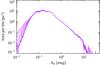 |
Fig. 1 Effect of 11 different boundaries used to derive the PDF of Orion B (dark: smaller area, light: larger area, by equal steps of ~4%). The effect on the PDF is almost exclusively confined to AK< 0.1 mag. |
As argued in the previous section, the PDF is expected to be affected by choice of cloud boundaries. Figure 1 shows how the histogram of the bin areas (thus essentially unnormalized PDFs) of Orion B changes when using different boundaries. As expected, this has a strong impact on AK< 0.1 mag, while the high end of the PDF is left unchanged.
As mentioned earlier, unrelated foreground or background material can contribute to the observed PDF. One way to correct for this is to look at the lowest extinction value in a large area around the cloud and to remove this amount from the extinction map (see also Schneider et al. 2015). Of course, this is a crude approximation since the subtracted column density is taken to be constant within the field. As a result, we expect “corrected” column densities to be affected by an additional noise equal to the average scatter of the superimposed material. This quantity, however, can be estimated (although approximately) by checking the off-field column density scatter and by applying a set of offsets that spans the same range in extinction. To test the bias associated with such a correction, we subtracted different extinction offsets to the PDF of Orion B. The result of this experiment (Fig. 2) demonstrates that this operation mostly affects the low end of the PDF: in particular, large offset corrections make the PDF peak broader (in a log-log plot) and move it to the left.
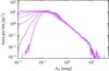 |
Fig. 2 Effect of 11 different offsets for the superposition bias correction in the PDF of Orion B (by steps of 0.02 mag). |
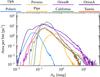 |
Fig. 3 Areas per extinction bin of different molecular clouds from Herschel/Planck dust-emission data. Bins span 0.01 dex. |
These simple tests demonstrate that the low end of the PDF is essentially unconstrained by the observations. We thus limit our investigation to the PDF at medium-to-high column densities. Figure 3 shows the raw histograms of bin areas for a set of molecular clouds, with boundaries selected from 2MASS/Nicest extinction maps (see Lombardi et al. 2006, 2008, 2010, 2011)2. We stress that using Planck data for the outskirts of the clouds was critical for investigating regions outside the Herschel coverage but still at relatively high values of extinction. Clearly there is a wide variety of PDF shapes, and in almost all cases there, they do not look like simple log-normal functions (which would appear as parabolae here). However, as discussed earlier, each cloud is affected by different levels of contamination due to unrelated foreground and background material. To remove this bias, we proceed as in Fig. 2 and subtract, for each cloud, a custom offset appropriately determined by careful examination of the outskirts of each object and list in Table1.
The result is shown as (normalized) PDFs in Fig. 4. Interestingly, many of the differences at AK ~ 0.1 mag to 0.5 mag evident in Fig. 3 are absent or mitigated in Fig. 4, suggesting that they are artificially induced by superposition of unrelated foreground and background material.
At extinctions >0.2 mag, the PDFs exhibit power-law shapes spanning approximately two decades with slopes ranging roughly between −4 and −2 (see Fig. 4 and Table1 where we list the indexes derived from a fit of the PDFs). In addition, they exhibit a turnover from a power law form near AK ~ 0.2 mag. Log-normal PDFs, which would appear as simple symmetric parabolae in these plots, are not evident for AK> 0.1 mag, with the possible exception of Polaris. Rather, it is evident that PDFs are very asymmetric in the log-log plot. Again, Polaris is a notable exception in this plot: it is more symmetric and displays a break at significantly lower column densities, as well as a steeper slope at the high extinction side. As argued above, the differences shown by clouds below AK ~ 0.1 mag are not significant; therefore, we cannot even assess whether there is a universal shape for the PDF in this regime, and in case there is, if the PDF is flat or increasing in this interval. Moreover, in this regime much of the measured extinction is likely to come from unrelated, more diffuse, atomic and molecular gas along the line of sight, rather than from the molecular cloud itself. At such low extinctions, it would be very difficult to separate any contribution to the intrinsic cloud PDF arising from a cloud’s own (more diffuse) outermost layers.
Extinction correction, the computed slopes n of the power law of the various clouds’ PDFs and the clouds’ Galactic latitudes b.
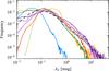 |
Fig. 4 PDFs of molecular clouds considered in this Letter, together with the PDF generated by a simple toy model (truncated isothermal profile, see Sect. 4) as a black dashed line. The PDFs have been corrected for the superposition bias by subtracting a constant offset to the dust extinction maps used to derive them. |
4. Discussion
Our inability to investigate the low end of the PDF limits our ability to distinguish different models for its shape. However, the data discussed in this Letter already provides enough information to draw some conclusions.
First, there is no indication that these PDFs are simple log-normal functions. Second, at high extinction, the PDFs are best described by power laws, with a break at AK ~ 0.15 mag. We observe that clouds with lower star formation activity (such as Polaris and Pipe) seem to be characterized by steeper slopes than more active star-forming clouds (such as Orion A and B, Ophiuchus, and Perseus). This is expected, since a steeper slope implies a lack of high-density material, hence reduced star formation activity (see Lombardi et al. 2013; and Lada et al. 2013). Interestingly, this result is consistent with recent simulations of turbulent cloud evolution that suggest that the slopes of the high extinction end of PDFs systematically vary with the age of the molecular cloud (Ward et al. 2014). In these simulations, Ward et al. find that an initially log-normal PDF develops a power-law tail that becomes increasingly prominent until it ultimately dominates the PDF above extinctions of AK ~ 0.2 mag. During this evolution the power-law indices systematically decrease with time, approaching a value of −2 after about 5 Myr. Although it is true that some portion of the PDF above 0.2 mag could still be fit by the arc of a broad log normal with a peak at lower extinctions (Alves de Oliveira et al. 2014; Ward et al. 2014), the observations simply require a function no more complicated than a power law in this regime. Unfortunately, the various biases present prohibit our ability to investigate the actual form of the cloud PDF below ~0.1 mag. Even though more complex models might account for, and be consistent with, a portion of the PDF above 0.2 mag, they are not required by the data. Thus, although other observations, such as cloud velocity fields, fractal boundaries, and scaling relations, may physically motivate turbulent cloud models, the observed PDFs by themselves cannot because in the regime where a log-normal distribution might exist, the intrinsic PDFs cannot be probed (see also Beaumont et al. 2012).
There is a clear indication that the power-law regime has a break at low values of extinction. Since the break is in an area that is still largely unaffected by the biases discussed in this Letter (see Fig. 1), we trust that the break is real. The location of the break coincides approximately with the column density required for CO self-shielding and is near the column density threshold for the H2-to-HI transition (AK ~ 0.04 to 0.1 mag; Sternberg et al. 2014; Planck Collaboration XIX 2011; Wolfire et al. 2010). This suggests that the break might be related to either or both of these thresholds. Also, the slope ~−2 of the power law is reminiscent of an isothermal profile (Lombardi et al. 2014). Therefore, it is reasonable to consider the PDF associated with a pressure-truncated isothermal profile to see if the associated PDF shares any similarity with the PDFs observed in real molecular clouds. We consider the toy model of truncated (singular) isothermal profile. The associated PDF can be provided in parametric form: 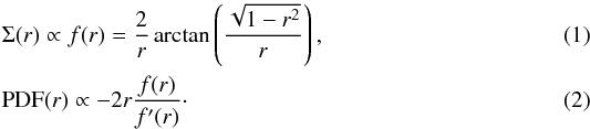 In this parametrization, r is the radius normalized to the truncation radius and Σ(r) the column density or extinction. In the limit of small r, substituting Eq. (1)in Eq. (2), we obtain PDF ∝ Σ-2. By plotting Eqs. (1)and (2), one sees that the function implicitly defined here broadly resembles the PDFs of many molecular clouds considered in this Letter (Fig. 4): this function has a slope of −2 for high column densities, and it peaks at the radius rbreak ≃ 0.72rtrunc, i.e., close to the truncation radius.
Of course, it is unrealistic to think that real clouds can follow spherically symmetric singular isothermal profiles exactly, with perfectly sharp outer edges. More naturally, an effective pressure truncation could result from a rapid increase in the local cloud sound speed, owing for example, to the transition from molecular to atomic gas or to a rapid increase in temperature or turbulence across the cloud boundaries. In the spherical approximation, AK ∝ Σ ∝ r-1 and the break of the PDF occurs at 1/0.72 ≃ 1.4 times the truncation column density. Since we observe the peak in the PDFs of many clouds at AK ~ 0.1 mag to 0.2 mag, we can argue that the truncation must occur around AK ~ 0.07 mag to 0.14 mag. As mentioned above, these values are not too far from the column density threshold for the H2-to-HI transition. (The exact location of this transition depends on several physical conditions of the cloud, such as the ultraviolet background and the exposure to cosmic rays.)
Another alternative is to imagine that molecular clouds can be (approximately) described as the sum of several isothermal spheres (for example, each corresponding a core). Individually, the PDF of each core would be a power law, and therefore the PDF of the entire cloud would also follow a power law. However, since the volume available for each core is limited (by the presence of the other cores), the resulting PDF shows a depression at low column densities with respect to the pure power law implied by (infinite) isothermal profiles. Therefore, this simple model could qualitatively explain the general shapes of the observed PDFs.
These interpretations are just a few of the several possible ones. Unfortunately, our inability to investigate the low end of the PDF makes it very difficult to distinguish among them. In particular, because of the intrinsic limitations of the column density measurements, presumed log-normal PDFs of clouds cannot be validated by such observations.
This is strictly true for dust extinction and emission studies. However, for relatively uncrowded regions, CO measurements have some power to remove this confusion using velocity information.
As discussed in the text, this figure is constructed directly from histograms of the logarithm of the column density map of each cloud, and differs by a simple scaling factor ∝ AK from Figs. 17 and 18 of Lombardi et al. (2014), which are constructed as derivative of the area function.
Acknowledgments
M.L. acknowledges financial support from PRIN MIUR 2010–2011, project “The Chemical and Dynamical Evolution of the Milky Way and Local Group Galaxies.”
References
- Alves, J., Lombardi, M., & Lada, C. J. 2014, A&A, 565, A18 [NASA ADS] [CrossRef] [EDP Sciences] [Google Scholar]
- Alves de Oliveira, C., Schneider, N., Merín, B., et al. 2014, A&A, 568, A98 [NASA ADS] [CrossRef] [EDP Sciences] [Google Scholar]
- Beaumont, C. N., Goodman, A. A., Alves, J. F., et al. 2012, MNRAS, 423, 2579 [NASA ADS] [CrossRef] [Google Scholar]
- Federrath, C., Roman-Duval, J., Klessen, R. S., Schmidt, W., & Mac Low, M.-M. 2010, A&A, 512, A81 [NASA ADS] [CrossRef] [EDP Sciences] [Google Scholar]
- Goodman, A. A., Pineda, J. E., & Schnee, S. L. 2009, ApJ, 692, 91 [NASA ADS] [CrossRef] [Google Scholar]
- Kainulainen, J., Beuther, H., Henning, T., & Plume, R. 2009, A&A, 508, L35 [NASA ADS] [CrossRef] [EDP Sciences] [Google Scholar]
- Kainulainen, J., Federrath, C., & Henning, T. 2014, Science, 344, 183 [NASA ADS] [CrossRef] [Google Scholar]
- Lada, C. J., Lombardi, M., Roman-Zuniga, C., Forbrich, J., & Alves, J. F. 2013, ApJ, 778, 133 [NASA ADS] [CrossRef] [Google Scholar]
- Lombardi, M. 2009, A&A, 493, 735 [NASA ADS] [CrossRef] [EDP Sciences] [Google Scholar]
- Lombardi, M., Alves, J., & Lada, C. J. 2006, A&A, 454, 781 [NASA ADS] [CrossRef] [EDP Sciences] [Google Scholar]
- Lombardi, M., Lada, C. J., & Alves, J. 2008, A&A, 489, 143 [NASA ADS] [CrossRef] [EDP Sciences] [Google Scholar]
- Lombardi, M., Lada, C. J., & Alves, J. 2010, A&A, 512, A67 [NASA ADS] [CrossRef] [EDP Sciences] [Google Scholar]
- Lombardi, M., Alves, J., & Lada, C. J. 2011, A&A, 535, A16 [NASA ADS] [CrossRef] [EDP Sciences] [Google Scholar]
- Lombardi, M., Lada, C. J., & Alves, J. 2013, A&A, 559, A90 [NASA ADS] [CrossRef] [EDP Sciences] [Google Scholar]
- Lombardi, M., Bouy, H., Alves, J., & Lada, C. J. 2014, A&A, 566, A45 [NASA ADS] [CrossRef] [EDP Sciences] [Google Scholar]
- Padoan, P., Jones, B. J. T., & Nordlund, A. P. 1997, ApJ, 474, 730 [NASA ADS] [CrossRef] [Google Scholar]
- Planck Collaboration XIX. 2011, A&A, 536, A19 [NASA ADS] [CrossRef] [EDP Sciences] [Google Scholar]
- Scalo, J., Vazquez-Semadeni, E., Chappell, D., & Passot, T. 1998, ApJ, 504, 835 [NASA ADS] [CrossRef] [Google Scholar]
- Schneider, N., André, P., Könyves, V., et al. 2013, ApJ, 766, L17 [NASA ADS] [CrossRef] [Google Scholar]
- Schneider, N., Ossenkopf, V., Csengeri, T., et al. 2015, A&A, 575, A79 [NASA ADS] [CrossRef] [EDP Sciences] [Google Scholar]
- Sternberg, A., Le Petit, F., Roueff, E., & Le Bourlot, J. 2014, ApJ, 790, 10 [NASA ADS] [CrossRef] [MathSciNet] [Google Scholar]
- Tassis, K., Christie, D. A., Urban, A., et al. 2010, MNRAS, 408, 1089 [NASA ADS] [CrossRef] [Google Scholar]
- Vazquez-Semadeni, E. 1994, ApJ, 423, 681 [NASA ADS] [CrossRef] [Google Scholar]
- Ward, R. L., Wadsley, J., & Sills, A. 2014, MNRAS, 445, 1575 [NASA ADS] [CrossRef] [Google Scholar]
- Wolfire, M. G., Hollenbach, D., & McKee, C. F. 2010, ApJ, 716, 1191 [NASA ADS] [CrossRef] [Google Scholar]
All Tables
Extinction correction, the computed slopes n of the power law of the various clouds’ PDFs and the clouds’ Galactic latitudes b.
All Figures
|
Fig. 1 Effect of 11 different boundaries used to derive the PDF of Orion B (dark: smaller area, light: larger area, by equal steps of ~4%). The effect on the PDF is almost exclusively confined to AK< 0.1 mag. |
| In the text | |
|
Fig. 2 Effect of 11 different offsets for the superposition bias correction in the PDF of Orion B (by steps of 0.02 mag). |
| In the text | |
|
Fig. 3 Areas per extinction bin of different molecular clouds from Herschel/Planck dust-emission data. Bins span 0.01 dex. |
| In the text | |
|
Fig. 4 PDFs of molecular clouds considered in this Letter, together with the PDF generated by a simple toy model (truncated isothermal profile, see Sect. 4) as a black dashed line. The PDFs have been corrected for the superposition bias by subtracting a constant offset to the dust extinction maps used to derive them. |
| In the text | |
Current usage metrics show cumulative count of Article Views (full-text article views including HTML views, PDF and ePub downloads, according to the available data) and Abstracts Views on Vision4Press platform.
Data correspond to usage on the plateform after 2015. The current usage metrics is available 48-96 hours after online publication and is updated daily on week days.
Initial download of the metrics may take a while.