| Issue |
A&A
Volume 576, April 2015
|
|
|---|---|---|
| Article Number | A17 | |
| Number of page(s) | 6 | |
| Section | Extragalactic astronomy | |
| DOI | https://doi.org/10.1051/0004-6361/201425563 | |
| Published online | 13 March 2015 | |
Research Note
A search for chaos in the optical light curve of a blazar: W2R 1926+42
1 Institute of Astronomy with NAO, Bulgarian Academy of Sciences, 1784 Sofia, Bulgaria
e-mail: bachevr@astro.bas.bg
2 Department of Physics, Indian Institute of Science, 560012 Bangalore, India
Received: 20 December 2014
Accepted: 5 January 2015
Aims. In this work we search for the signatures of low-dimensional chaos in the temporal behavior of the Kepler-field blazar W2R 1946+42.
Methods. We use a publicly available, ~160 000-point-long and mostly equally spaced light curve of W2R 1946+42. We apply the correlation integral method to both real datasets and phase randomized surrogates.
Results. We are not able to confirm the presence of low-dimensional chaos in the light curve. This result, however, still leads to some important implications for blazar emission mechanisms, which are discussed.
Key words: chaos / BL Lacertae objects: general / BL Lacertae objects: individual: W2R 1946+42
© ESO, 2015
1. Introduction
Within the large family of active galactic nuclei (AGN), blazars are the only members whose emission is produced primarily in a relativistic jet via synchrotron and inverse-Compton processes. To be identified as a blazar, the jet should be oriented at a small angle to the line of sight. The blazar spectral energy distribution (SED) consists of two peaks: a synchrotron one that usually peaks in the optical region, and an inverse-Compton one, peaking in the X/γ-ray region.
Like most of the other AGN types, blazars are known to be highly variable in the optical. In fact, they are the only AGN class for which evidence of significant variations clearly exists even on intranight time scales (Bachev et al. 2012, and the references therein). Blazar optical variability (i.e., the synchrotron peak variability) on long-term time scales can generally be described as unpredictable and lacking any periodicity (see, however, e.g. Gupta et al. 2009). In spite of the extensive studies throughout the years, no clear reason for such blazar variations has been positively identified. Unlike the radio-quiet AGN, where accretion disk instabilities are usually invoked to account for the variations, the blazar case requires that similar “variability drivers” be searched for in the processes taking place in a relativistic jet. They range from purely geometrical ones (changing the Doppler factor of the emitting blob and/or microlensing from intervening foreground objects) to a complex evolution of the relativistic particles’ energy distribution (interplay between particle acceleration and synchrotron or inverse-Compton losses). In any case, studying blazar light curves may provide a better clue to the physics of the relativistic jets, provided sufficient data are available.
A way to explore apparently random and non-periodic time series is to search for low-dimensional deterministic chaos, which may allow a purely stochastic process to be distinguished from a process driven by a nonlinear (and presumably chaotic) dynamical system. While the former case most likely implies the presence of many factors acting independently (e.g., many independent emitting components), the latter suggests that the entire system might be governed by a small (say 3−5) number of degrees of freedom.
One approach to search for low-dimensional chaotic signatures in a time series is to apply the correlation integral (CI) method (Grassberger & Procaccia 1983, see also Sect. 2.2). In the past, similar analyses have been performed for AGN on EXOSAT X-ray light curves of several, mostly radio-quiet objects, leading to no conclusive results (Lehto et al. 1993), perhaps owing to the insufficient number of data points, ranging from ~300 to ~4000 for the different sources, as well as to the relatively larger photometric uncertainty.
No conclusive results for the presence of low-dimensional chaos have been obtained either for 3C 345 (Provenzale et al. 1994), based on the 800-point-long optical dataset with linearly interpolated missing parts. Indications of the possible fractal nature of the light curves of a few other blazars were found by Marchenko & Hagen-Thorn (1997); however, again – huge missing parts of the light curves were replaced by means of interpolation. Nonlinear (and perhaps chaotic) variability has been found by Gliozzi et al. (2002) in a 10 000-point X-ray light curve of Akn 564, a radio-quiet AGN observed by Ginga satellite. Chaotic signatures in ~ 20 000-point-long light curves in the X-ray binary GRS 1915+105 (Misra et al. 2004) was also reported.
Dataset description.
As mentioned above, most of the previous work has focused on Seyfert 1 galaxies, whose observed properties are very different from those of BL Lacs. For example, BL Lacs are very rapidly variable, highly polarized, often exhibit superluminal motion and emit up to TeV energies, while Seyfert 1-s do not exhibit such properties. Moreover, the physics is also believed to be different between them: beamed versus relatively isotropic emission.
In this paper, we apply the correlation integral method to search for low-dimensional chaotic signatures in the optical light curve of W2R 1926+42 – a blazar within the Kepler satellite field (Edelson et al. 2013). This object has by far the largest-ever optical dataset (consisting of almost 160 000 data points in total), owing to the unique Kepler capability of repeatedly observing the same field. More importantly, large segments of equispaced data are available, which is specifically required by the CI method. In this work, to the best of our knowledge, the CI analysis is applied for the first time on such a large equidistant optical dataset of a blazar. Figure 1 shows the entire light curve of W2R 1926+42. Clearly, the object shows rapid and significant variability over five times in terms of count rates, allowing a formal distinction of “low” and “high” states, which will be treated separately later in our analysis.
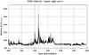 |
Fig. 1 Long-term light curve of W2R 1926+42 from Kepler. |
The plan of the paper is the following. In the next section, we describe the dataset under consideration and the CI method used. Subsequently, we discuss the method followed to search for chaos in data and results in Sect. 3 and present a discussion in Sect. 4. Finally, we end with a summary in Sect. 5.
2. Search for chaos
2.1. Dataset
W2R 1926+42 (19:26:31 +42:09:59, z = 0.155) is a BL Lac (an “LBL”, Padovani & Giommi 1995) object that happens to fall in the Kepler satellite field (Edelson et al. 2013). The Kepler continuous monitoring covers a time period of about 1.6 years (quarters 11 through 17), starting 29 September 2011, with a sampling of about 30 min and a duty cycle of about 90%. The typical photometric errors are less than 0.002%. From all available datasets, we identified 18 uniformly sampled segments of lengths ranging from about 1300 to about 16 000 points (PDCSAP_FLUX data, covering roughly the 4300−8900 Å range). Occasionally, where some data points (one rarely up to five) are missing, those are replaced by of linear interpolation, since the CI method requires equidistant sampling. For longer missing parts, the entire dataset had to be divided into separate segments. Any remaining parts with lengths less than of 1000 points (if such) are not considered in this analysis.
Although covered by long cadence datasets (“llc”), the short cadence data (“slc”, sampling of about a minute) are treated separately because they provide a much larger time resolution and dataset length. For the short cadence datasets where photometric errors are larger (up to 0.02%), a median filter is applied over every three data points. This procedure helps to largely reduce some spurious effects of significantly deviating single points and to reduce almost twice the photometric error value, of course with the price of reducing the dataset lengths. The data segments used in this analysis are given in Table 1. The start and end times are in days (BJD-2 454 833) and N is the number of the points in the segment.
2.2. Tests
The solution of a nonlinear dissipative dynamical system is known as attractor, if it stays bound within a finite volume of the phase space (e.g., Lorenz attractor; Lorenz 1963). An attractor is strange, if it has a noninteger dimension. The trajectories of a strange attractor evolve in a finite volume of the phase space, never returning to the same point. The divergence between two infinitesimally close trajectories increases exponentially in time making the long-term predictions impossible.
The CI method is a suitable approach for revealing signatures of low-dimensional chaotic behavior in time series data (Vio et al. 1992). The method relies on constructing a new (empirical) phase space from the available N discrete data points. The dataset (e.g., the light curve) is separated into segments of length d. Each segment can be considered as a d-dimensional vector (Xi), embedded in the d-dimensional empirical phase space. The number of the vector pairs within a distance below r is computed as a function of r for different d and related to the total number of pairs (np) for that d. Thus, the correlation integral can be expressed as
where Θ is the Heaviside′s function. Therefore, if the dimension of the attractor is D, then
 Increasing the embedded dimension d therefore leads to saturation when d>D, which can be used for estimating the attractor dimension
 where Dc is the correlation dimension of the attractor and can be a noninteger value. Knowledge of Dc allows determining the number of differential equations, thus describing the dynamical system, N, which is the first integer value, larger than Dc and therefore makes it possible to draw conclusions about the physical process driving the variability.
The so-called Ruelle’s criterion (Ruelle 1990) relates the maximum dimension of an attractor (if present), that can be detected from a time series of N points, with N itself as Dmax ≤ 2log N, which in our case means Dmax = 6 − 8, depending on the segment.
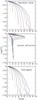 |
Fig. 2 CI diagrams for random noise (upper panel), Lorenz attractor (middle panel), and phase-randomized Lorenz attractor surrogate (lower panel). For presentation purposes, different embedded dimensions, d = 1,2,...10 (from left to right) are shown in different colors. |
As pointed out by Lehto et al. (1993), the results from the CI method might be significantly contaminated if a strong periodic component (D = 1) is present in the data. Broadly speaking, false results of chaotic signatures might be an artifact of the exact shape of the power-density spectrum (PDS) of the dataset. Therefore, one should also perform the CI test on surrogate data, that is, what has been generated from the original data PDS after phase-randomization (Schreiber & Schmitz 1996; Karak et al. 2010). If the chaotic signature of the original time series is real, this should not be present in the surrogate.
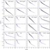 |
Fig. 3 CI diagrams for different segments of the blazar light curve for different embedding dimensions, same as in Fig. 2: the last 3 digits of the dataset (see Table 1) are indicated. The upper panel of each box is for the real dataset, the lower one is for the phase-randomized surrogate. None of the diagrams shows clear indication for a strange attractor of low dimension, especially considering that the “surrogate” diagrams are very similar to the ones of the real data. |
3. Results
Before applying the CI method to real data, we tested it with light curves of known correlation dimension. Figure 2 (upper panel) shows the results for a 1500-point-long random noise light curve (infinite dimension). The figure shows the variation of log CI with its slope dlog CI/ dlog r, for different embedded dimensions (d = 1...10), each presented by a separate curve (of different color in the electronic version). As one sees, each embedded dimension saturates at its corresponding value, indicating that there is no low-dimensional attractor in these data, as expected. Next (Fig. 2, middle panel) is for a 1500-point-long Lorenz attractor light curve (Dc = 2.06). Here all embedded dimensions of d> 2 saturate around 2.06, indeed revealing the presence of a low-dimensional attractor. Finally, in the lower panel of Fig. 2, we see the results for the same Lorenz light curve, this time phase-randomized (surrogate data). As expected, no long dimensional saturation can be seen, meaning that phase randomization destroys the attractor (provided such is present, which is the case for a Lorenz attractor).
This simple test suggests that if a low-dimensional attractor is really present in the original dataset, it should not be seen in the phase-randomized surrogates; i.e., both log CI versus dlog CI/ dlog r plots should differ significantly.
Figure 3 shows CI diagrams for different segments of the blazar light curve. Although the pattern does not resemble the one of the pure random noise, we cannot find any evidence of saturation (i.e., the presence of a low-dimensional attractor) in any of the segments. Since we have only tested for the first ten embedded dimensions, one can conclude, based on this test, that the correlation dimension (also very similar to the so-called fractal dimension) could indeed be greater than 10. However, the goal usually is to find “low” dimensional chaos with D ~ 3−4, which may indeed be useful for constraining or developing the theory, as discussed below. Furthermore, the surrogates show very similar patterns to the real datasets, meaning that any peculiarity should be attributed to the particular structures in the light curve PDS. Actually, the results are somewhat similar to those reported by Lehto et al. (1993) for their shot-noise model, as well as for most of the sources they studied, even though the emission mechanisms in these two (blazar and non-blazar) types of objects are very different.
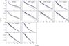 |
Fig. 3 continued. |
4. Discussion
Finding low-dimensional behavior in a dynamical system (in our case, a light curve) can be hugely important for the theoretical models, because it may limit the number of independent variables (or the number of equations) that governs the system entirely. People often invoke the so-called single-zone model to reproduce the observed blazar SED. In this model the synchrotron radiation, which is responsible for the optical emission, is controlled by only a few parameters – electron density, magnetic field, Doppler factor, etc. Therefore, if the single-zone models actually work most of the time, one should expect to find low-dimensional (say D ≃ 3 − 4) behavior in blazar light curves.
Indeed, the electron energy density evolution due to external injection and (synchrotron and synchrotron self-Compton, SSC) radiation losses is described by the Fokker-Planck (kinetic) equation (Kardashev 1962): ![\begin{eqnarray*} \frac{\partial n(\gamma,t)}{\partial t} = \frac{\partial }{\partial \gamma}\left[|\dot{\gamma}_{\rm tot}|n(\gamma,t) \right] + S(\gamma,t) \end{eqnarray*}](/articles/aa/full_html/2015/04/aa25563-14/aa25563-14-eq34.png) where n(γ,t) is the relativistic-particle energy distribution,
where n(γ,t) is the relativistic-particle energy distribution,  is the total loss and S(γ,t) is the energy injection (source) term. The synchrotron spectrum (at least its optical part) is entirely determined by n(γ,t) (e.g., Tsang & Kirk 2007, Appendix A). In a case of a single monochromatic injection (as frequently assumed), the solution of the kinetic equation is “trivial” in the sense that it cannot account for the intermittent blazar variability (Fig. 1).
The energy injection (particle acceleration) mechanism is generally unknown; however, if the injection occurs near the jet base it might be considered deterministic in nature, rather than completely stochastic. The reason for this assumption is that in such a case the accretion flow and/or black hole properties (such as spin) should control the relativistic particle acceleration entirely. Deterministic injection will perhaps lead to deterministic optical variability, evidence of which we did not find from our results.
One way to account for the apparently stochastic light curves, which would be consistent to a grater extent with our findings, is to invoke a large number of active zones (emitting blobs). The overall light curve in this case will be stochastic in nature, independently of the exact injection mechanism in each zone.
One such mechanism is based on magnetic reconnections that may occur within the jet and accelerate electrons locally to relativistic energies, thus leading to variability that is intermittent and stochastic in nature. The light curve will perhaps be similar to the shot noise case – i.e., randomly distributed in time and amplitude explosive events (flares) possibly with different characteristic times. The flares can occur completely at random or can be a representation of the so-called self organized criticality (SOC), i.e. when one reconnection may lead to an avalanche of subsequent reconnections (see Aschwanden 2014, for a recent review). The latter possibility is supported by the often-reported 1 /f shape of the blazar PDS’s.
Another way to account for the observed variability is to invoke the presence of turbulence in the jet. In these models either turbulent flow passes through a standing shock (e.g., Marscher 2014) leading to instant energy injection in the corresponding (shock crossing) plasma volume or the opposite: a shock wave passes though a turbulent medium (Marscher et al. 1992; Kirk et al. 1998). The turbulent flow in these works is modeled as an ensemble of cells with different properties (randomly distributed within certain limits), which will naturally lead to stochastic overall variability. This approach, however, might be an oversimplification of turbulence. Although no fully developed theory of turbulence exists, turbulence and chaos seem to be deeply related (Procaccia 1984). In fact, low-dimensional fractal structures have been found in turbulent jets in lab experiments (Zhao et al. 2008), so if turbulence is playing a major role in shaping blazar jets, one might expect to witness not only fractal spatial structure but perhaps also fractal temporal behavior (i.e., low-dimensional chaos in the light curves). On the other hand, depending on the exact shock geometry and line-of-sight angle, light crossing time delays between emitting cells might be expected (Marscher 2014), which may somehow affect the overall light curve and eventually conceal the presence of low-dimensional chaos. But as we stressed above no fully developed turbulence theory is available, so it is difficult to judge whether a turbulent blazar jet should manifest chaotic temporal behavior or not.
It is interesting to note that there is no practical difference between the CI diagrams for segments covering the high states and the low states of the light curve. One would normally think that for the low states, there should be fewer active regions (perhaps even only one), contributing to the emission. If there were many independent regions contributing to the emission, it would be unlikely to find a low-dimensional attractor in the light curve. On the other hand, it would be more likely to find it if a single zone (of a very few) is generating the energy. Not finding a difference in the CI diagrams means there is perhaps no huge difference in the number of zones for low and high states (i.e., when a significant number in both cases). Another explanation, of course, is that the temporal evolution of a single zone is too stochastic to be described in terms of low-dimensional chaos. Or maybe the entire picture of the blazar emission generation is more complex than we have previously thought.
5. Summary
We have applied the CI method to the longest-ever available dataset of a light curve of a Kepler blazar – W2R 1946+42 to search for signatures of low-dimension chaotic behavior. Our results do not reveal this for any of the segments, which cover both high and low states of the blazar.
Although not entirely conclusive, these results may suggest the mechanism of particle acceleration. Models, based on a “single engine” that operates perhaps close to the jet base seem unlikely. Models that rely on the presence of many independent active zones, such as multiple magnetic reconnections or turbulence within the jet, are plausible.
Further tests are, however, required for a firm conclusion.
Acknowledgments
This paper is supported by Bulgarian National Science Fund through grant NTS BIn 01/9 (2013) and an Indo-Bulgarian Project funded by Department of Science and Technology, India, with grant No. INT/BULGARIA/P-8/12.
References
- Aschwanden, M. 2014, ApJ, 782, 54 [NASA ADS] [CrossRef] [Google Scholar]
- Bachev, R., Semkov, E., Strigachev, A., et al. 2012, MNRAS, 424, 2625 [NASA ADS] [CrossRef] [Google Scholar]
- Edelson, R., Mushotzky, R., Vaughan, S., et al. 2013, ApJ, 766, 16 [NASA ADS] [CrossRef] [Google Scholar]
- Gliozzi, M., Brinkmann, W., Räth, C., et al. 2002, A&A, 391, 875 [NASA ADS] [CrossRef] [EDP Sciences] [Google Scholar]
- Grassberger, P., & Procaccia, I. 1983, Phys. Rev. Lett., 50, 448 [Google Scholar]
- Gupta, A. C., Srivastava, A. K., & Wiita, P. J. 2009, ApJ, 690, 216 [NASA ADS] [CrossRef] [Google Scholar]
- Karak, B., Dutta, J., & Mukhopadhyay, B. 2010, ApJ, 708, 862 [NASA ADS] [CrossRef] [Google Scholar]
- Kardashev, N. S. 1962, Sov. Astron. J., 6, 317 [NASA ADS] [Google Scholar]
- Kirk, J. G., Rieger, F. M., & Mastichiadis, A. 1998, A&A, 333, 452 [NASA ADS] [Google Scholar]
- Lehto, H., Czerny, B., & McHardy, I. 1993, MNRAS, 261, 125 [NASA ADS] [CrossRef] [Google Scholar]
- Lorenz, E. N. 1963, J. Atm. Sci., 20, 130 [Google Scholar]
- Marchenko, S. G., & Hagen-Thorn, A. V. 1997, Astrophys., 40, 222 [NASA ADS] [CrossRef] [Google Scholar]
- Marscher, A. P. 2014, ApJ, 780, 87 [NASA ADS] [CrossRef] [Google Scholar]
- Marscher, A. P., Gear, W. K., & Travis, J. P, 1992, in Variability of Blazars, eds. E. Valtaoja, & M. Valtonen (Cambridge Univ. Press), 85 [Google Scholar]
- Misra, R., Harikrishnan, K. P., Mukhopadhyay, B., Ambika, G., & Kembhavi, A. K. 2004, ApJ, 609, 313 [NASA ADS] [CrossRef] [Google Scholar]
- Padovani, P., & Giommi, P. 1995, ApJ, 444, 567 [NASA ADS] [CrossRef] [Google Scholar]
- Procaccia, I. 1984, J. Stat. Phys., 36, 649 [NASA ADS] [CrossRef] [Google Scholar]
- Provenzale, A., Vio, R., & Cristiani, S. 1994, ApJ, 428, 591 [NASA ADS] [CrossRef] [Google Scholar]
- Ruelle, D. 1990, in Deterministic chaos: the science and the fiction, Proc. R. Soc. Lond., 427, 241 [NASA ADS] [CrossRef] [Google Scholar]
- Schreiber, T., & Schmitz, A. 1996, Phys. Rev. Lett., 77, 635 [NASA ADS] [CrossRef] [PubMed] [Google Scholar]
- Tsang, O., & Kirk, J. G. 2007, A&A, 463, 145 [NASA ADS] [CrossRef] [EDP Sciences] [Google Scholar]
- Vio, R., Cristiani, S., Lessi, O., & Provenzale, A. 1992, ApJ, 391, 518 [NASA ADS] [CrossRef] [Google Scholar]
- Zhao, Y. X., Yi, S. H., Tian, L.F., He, L., & Cheng, Z. Y. 2008, Sci. China Ser. G., 51, 1134 [CrossRef] [Google Scholar]
All Tables
All Figures
|
Fig. 1 Long-term light curve of W2R 1926+42 from Kepler. |
| In the text | |
|
Fig. 2 CI diagrams for random noise (upper panel), Lorenz attractor (middle panel), and phase-randomized Lorenz attractor surrogate (lower panel). For presentation purposes, different embedded dimensions, d = 1,2,...10 (from left to right) are shown in different colors. |
| In the text | |
|
Fig. 3 CI diagrams for different segments of the blazar light curve for different embedding dimensions, same as in Fig. 2: the last 3 digits of the dataset (see Table 1) are indicated. The upper panel of each box is for the real dataset, the lower one is for the phase-randomized surrogate. None of the diagrams shows clear indication for a strange attractor of low dimension, especially considering that the “surrogate” diagrams are very similar to the ones of the real data. |
| In the text | |
|
Fig. 3 continued. |
| In the text | |
Current usage metrics show cumulative count of Article Views (full-text article views including HTML views, PDF and ePub downloads, according to the available data) and Abstracts Views on Vision4Press platform.
Data correspond to usage on the plateform after 2015. The current usage metrics is available 48-96 hours after online publication and is updated daily on week days.
Initial download of the metrics may take a while.