| Issue |
A&A
Volume 576, April 2015
|
|
|---|---|---|
| Article Number | A132 | |
| Number of page(s) | 14 | |
| Section | Numerical methods and codes | |
| DOI | https://doi.org/10.1051/0004-6361/201424801 | |
| Published online | 20 April 2015 | |
Determining spectroscopic redshifts by using k nearest neighbor regression
I. Description of method and analysis
Heidelberger Institut für Theoretische Studien (HITS), Schloss-Wolfsbrunnenweg 35 69118 Heidelberg Germany
e-mail:
dennis.kuegler@h-its.org
Received: 13 August 2014
Accepted: 6 February 2015
Context. In astronomy, new approaches to process and analyze the exponentially increasing amount of data are inevitable. For spectra, such as in the Sloan Digital Sky Survey spectral database, usually templates of well-known classes are used for classification. In case the fitting of a template fails, wrong spectral properties (e.g. redshift) are derived. Validation of the derived properties is the key to understand the caveats of the template-based method.
Aims. In this paper we present a method for statistically computing the redshift z based on a similarity approach. This allows us to determine redshifts in spectra for emission and absorption features without using any predefined model. Additionally, we show how to determine the redshift based on single features. As a consequence we are, for example, able to filter objects that show multiple redshift components.
Methods. The redshift calculation is performed by comparing predefined regions in the spectra and individually applying a nearest neighbor regression model to each predefined emission and absorption region.
Results. The choice of the model parameters controls the quality and the completeness of the redshifts. For ≈90% of the analyzed 16 000 spectra of our reference and test sample, a certain redshift can be computed that is comparable to the completeness of SDSS (96%). The redshift calculation yields a precision for every individually tested feature that is comparable to the overall precision of the redshifts of SDSS. Using the new method to compute redshifts, we could also identify 14 spectra with a significant shift between emission and absorption or between emission and emission lines. The results already show the immense power of this simple machine-learning approach for investigating huge databases such as the SDSS.
Key words: methods: data analysis / astronomical databases: miscellaneous / methods: statistical / galaxies: distances and redshifts / catalogs
© ESO, 2015
1. Introduction
In the past decades, the rapidly increasing amount of available data has been one of the greatest challenges in astronomy. In contrast to the amount of data, the number of techniques and the knowledge of how to analyze these large data sets has only increased slowly over time. When the first digital, photometric all-sky surveys were performed, the amount of available data was already too large to be inspected manually. With the advent of spectroscopic surveys and additional photometric surveys in multiple wavelengths, the available data volume increased so rapidly that novel approaches are mandatory.
So far, the most successful survey in astronomy has been the Sloan Digital Sky Survey (SDSS, York et al. 2000), which in its current 10th data release (DR10, Ahn et al. 2014) contains photometry for one billion objects and spectra covering the near-UV to the near-IR for roughly three million objects. In the future, surveys such as the Large Sky Area Multi-Object Fiber Spectroscopic Telescope (LAMOST, Cui et al. 2012) will reach this amount of data in a fraction of the time needed by SDSS. Thus more advanced techniques for handling those immense data streams have to be developed.
The determination of spectral redshifts and classifications of the SDSS spectra is based on template fitting. Therefore generalized templates are created by combining spectra of similar objects for all empirically determined classes of objects. By fitting those templates to the spectra, a number of predefined properties, such as redshift, can be individually computed for every object. The best fitting template is determined by applying all available templates to the data while allowing for some variation in a set of parameters (e.g. width of features) and testing the reliability of every model by computing a reduced χ2. Instead of using the full information available, just a simplified model with a limited flexibility is applied, which does not allow a more detailed discussion of individual properties. Furthermore, the choice of the reference spectra and the creation of these templates have a strong impact on the determined properties.
With this publication we want to emphasize the power of statistical learning in huge spectral databases. From here on, “huge” refers to a large number of entities and dimensions. While this approach can in principle be applied to any database, we focus on SDSS. There are many applications of machine-learning techniques in astronomy (see Borne 2009; Ball & Brunner 2010). So far, spectroscopically derived properties have mainly been used as ground truth to estimate redshifts on photometric data, for example in Laurino et al. (2011), Gieseke et al. (2011), Polsterer et al. (2013). In contrast less attention has been paid to the application of machine learning to the spectral data itself (see Richards et al. 2009; Meusinger et al. 2012), which can be mainly attributed to the “curse of dimensionality” (see Bellman & Bellman 1961). The ultimate goal would be to obtain spectral properties that are not based on the created templates but rather on the rich experience existing in the database instead.
The algorithm presented in this paper will perform a consistency check of the redshift calculated by the SDSS pipeline. We therefore assume that the majority of the spectra is fairly well described by one of the templates, so the redshift is determined to be reasonably precise. Of course the templates do not describe all kinds of objects perfectly, thus at least some will be misfit. The great improvement in calculating redshifts based on a data-driven approach is that the redshifts can be determined model-independent. This method is suitable for determining redshifts of unknown spectra and in a forth-coming paper we will present a value-added catalog of redshifts to the existing SDSS spectra. In this paper we focus on the technical side and explain the impact of the choice of different model parameters. To highlight the power of this new method, some outliers in terms of redshift in the used subsample are presented. The motivation for employing new methods for redshift computation is manifold:
-
1.
Validation: cross-validating the self-consistency of the computed redshifts is crucial for understanding caveats of the SDSS pipeline. The independent determination of a redshift increases the confidence and the number of reliable redshifts.
-
2.
Calculating redshifts: we are able to determine model-independent redshifts of existing and future spectra with high precision. This is possible since we are determining the redshift as an ensemble property and thus the theoretical resolution can be improved statistically with the number of similar spectra in the reference database, as well as with the dimension of the feature vector.
-
3.
Rare objects: many different attempts have been performed to find rare objects showing shifts between spectral features in the SDSS spectral database (see Bolton et al. 2004; Tsalmantza et al. 2011). With the presented method we will be able to detect more of those since our method can deal with lower signal-to-noise ratio (S/N) than with template fits.
-
4.
Unexpected behavior: this can be caused by objects of a previously unknown class or by a superposition of two classes. Those objects might possibly be the science drivers in the near future. Also, artifacts in the reduction pipeline/in the data can be discovered.
The paper is structured as follows. Section 2 describes the data used for creating and testing our model. In Sect. 3 we explain the basic approach used in our method in more detail. In Sect. 4 we discuss the performance of our method in terms of precision and reliability. Also some outliers and peculiar objects are discussed in more detail. A summary and an outlook follow in Sect. 5. In a follow-up paper, we describe the value-added catalog that gives redshifts for all available objects based on specific spectral regions. Additionally, a catalog containing all detected outliers will be presented there.
2. The SDSS spectroscopic database
For testing our method, we are analyzing the spectroscopic database of SDSS. This survey uses a dedicated 2.5 m mirror telescope located at the Apache Point Observatory (New Mexico, USA) to map the northern galactic cap and is a joint project by USA, Japan, Korea, and Germany.
The telescope was first used to image different stripes of the northern hemisphere in five filter bands using the drift scan method. Subsequently, interesting objects were selected by brightness limits and different color cuts for spectroscopy (R = λ/ Δλ ≈ 2000) with 3600 Å ≤ λ ≤ 10 000 Å (Eisenstein et al. 2001; Richards et al. 2002; Strauss et al. 2002). Those selection criteria have a direct impact on the quality of reference sample. In the current DR10 (Ahn et al. 2014) more than three million spectra were taken of which far more than two million are nonstellar sources according to the SDSS-classification.
It is important to mention that depending on the applied learning technique, a large number of reference objects with a representative sampling is mandatory. With millions of objects, the SDSS is more than sufficiently large1.
2.1. Data calibration/SDSS pipeline
As mentioned in the caveats of SDSS, the night sky subtraction can suffer from severe inaccuracy by rapidly changing conditions, e.g., auroral activity. Thus the night sky subtraction leaves a severe signature in some of the spectra, which is sometimes not taken into account correctly in the error estimation. As a consequence, faint features in the vicinity of strong night sky emission lines might be artifacts. The spectra are automatically labeled, both flux- and wavelength-calibrated, and eventually combined with potentially pre-existing observed spectra of the same object.
In a second step, the calibrated spectra were processed via an identification pipeline that assigned a redshift, a classification, and a velocity dispersion to the individual spectra (Bolton et al. 2012). The classification and redshift determination was performed with a principal component analysis (PCA) of a rest-frame shifted training sample. A linear combination of eigenspectra were then shifted with respect to flux and wavelength until a minimal residual was reached. The precision of the redshift for a single line is limited by the resolution per pixel (~ 100 km s-1) of the spectrograph but can be improved by computing it independently for all lines that are available. This method is extremely efficient for spectra that show the expected behavior and as confirmed by performing a self-consistency check later on, and the quality of the SDSS redshifts has high reliability.
2.2. Reference and test sample
The analysis of the method was performed on a small subsample of the SDSS data in order to make the different model and parameter evaluations computationally feasible. The analysis of the algorithm is limited to the plates 0266 to 0289, including the exposures of all modified Julian dates (MJDs). Additionally, the sample was restricted to the redshift range between 0.01 ≤ z ≤ 0.5. The selected restriction allows a more reliable prediction of the regression value because the density of reference targets in the direct neighborhood is sufficiently high. The chosen subsample includes 16 049 spectra in total. The redshift distribution of the spectra can be found in Fig. 1. In the following, this sample is used as reference and test set at the same time; that is, we will perform a leave-one-out cross validation. That means that all but the target spectrum are reference spectra. Since we are only able to compute redshifts within the covered feature space, under-represented objects (high-redshifted galaxies, QSO) will yield worse redshifts than normally represented redshifts.
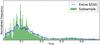 |
Fig. 1 Comparison of the redshift distribution of the selected subsample (green) and the entire SDSS (blue). There is a steep drop in the frequency toward redshifts z> 0.25. Single redshift bins are apparently undersampled. |
3. Applied method
The basic idea for determining the spectroscopic redshift z is to perform a comparison between similar objects. This is done by finding objects that look similar in terms of Euclidean distance and then computing the regression value of the unknown target by comparing it to the redshifts of the most similar spectra.
To be able to compare the spectra, instead of using the plain SDSS spectra we have to pre-process them. The method is a purely data-driven approach without deriving a generalization, and thus the quality of the redshifts relies directly on the chosen reference sample. While this seems contradictory on first sight, the method performs comparably on a smaller but representative reference set. It is obvious that the choice of a representative reference sample can only be obtained when domain-knowledge is included. Limiting the reference sample in redshift space would limit the derived values, respectively.
3.1. k nearest neighbor regression
Our method is based on k nearest neighbor (kNN) regression, which is a commonly used technique in statistical learning (Hastie et al. 2009). All spectra have d datapoints (corresponding to the individual flux measurements in the spectra) and are thus members of a d-dimensional feature space. The reference sample ℛ consists of m entities and corresponds to the number of reference spectra from which the model learns, 16 048 in this case. Mathematically this sample can be described with  (1)where
  is the ith d-dimensional input vector (spectrum under consideration) corresponding to the flux value in each pixel, and yi is the redshift value z assigned by the SDSS pipeline.
The kNN regression is based on calculating similarities in the d-dimensional feature space. For any d-dimensional feature vector  , the similarity to a reference object can be estimated with distance measure
  . The most commonly used metrics are
  The impact of the choice of the metric on the final results was only marginal. Therefore we only use the common Euclidean distance. In general, the neighborhood
  is determined on the basis of the representation of the reference objects in the feature space, such that
  (2)however, here we make use of a modified version:
  (3)Different algorithms exist for finding the k most similar spectra . The most straight-forward one is the brute-force method where each spectrum is simply compared to each of the others and the distance is computed. In contrast, spatial structures exist (kd-, ball-trees) that are able to structure the data in advance. The average time to find the closest spectra is thus significantly lower once the search structure is created. When experimenting with spatial trees, we learned that the dimension of our data is apparently so high and the data themselves are so unstructured that spatial trees do not perform significantly better than the brute-force method, and as a consequence only the brute force method is used throughout the paper and for the future catalog.
The considered kNN regression is limited to interpolating values within the reference sample. As a consequence, redshifts of objects with extremely high redshift or very peculiar spectral features cannot be determined correctly.
3.2. Requirements
The method of kNN regression can only work efficiently if the following requirements are met:
-
1.
The majority of the redshift determinations by SDSS is correct. In the following the deviation of the SDSS redshifts in comparison to the correct redshift is assumed to be small. This is verified by comparing our results to the redshifts determined by SDSS. One has to keep in mind that for a large fraction of the data, the template fitting works quite well, and the redshifts are fairly reliable.
-
2.
The number of objects in the reference data set is large compared to the dimensionality. This is already met in our test subsample. Nonetheless this is quite surprising because the number of entities is approximately the number of dimensions (4000). It appears that the multidimensional feature space is sufficiently homogeneously populated with reference objects. Applying this method to the entire database will just strengthen that assumption further.
-
3.
It is possible to distinguish noise from real signals for most of the data. This requirement is harder to meet because the distinction between signals and noise, especially for low S/N spectral lines, has always been a huge challenge for astronomers. In this work, we use an approach that is based on a simple similarity measure used by the type of the applied regression method. The basic assumption is that when a detectable line exists anywhere in the spectrum, it should be possible to find similar spectra that, within their errors, have a similar redshift. Those form a sharp distribution around the real value. On the other hand, a spectrum that contains pure noise will yield an even distribution of redshift values over the entire tested redshift range, and thus the average deviation from the median or mean will be quite high. In the distribution of so-called errors, which correspond to the deviation of reference redshifts across similar spectra, one would naively expect a superposition of two behaviors. The dominant component is a distribution that shows a drop toward higher deviations with a width that is comparable to the sensitivity of the method. This distribution corresponds to redshifts based on true absorption or emission lines. Underlying the first component there is a flatter distribution that represents the spectra that contain mostly noise. This is discussed further in Sect. 4.
3.3. Preprocessing
The preprocessing is needed to make the spectra comparable. Effects like apparent brightness are not important, since we are interested solely in absorption and emission features, therefore the behavior of the continuum has to be estimated and subtracted.
3.3.1. Regridding
The dispersion resolution between different fibers on a single plate and between the plates themselves differ slightly. To always be able to compare the correct wavelength bins, which do not exactly agree with redshift bins, the spectra have to be regridded. We therefore create a global grid that is defined by  (4)where λ is the wavelength in Å for a given pixel position p, with 0 ≤ p< 5100. The parameters of the function are chosen such that the dispersion solution corresponds to the average of our selected subsample. The regridding is performed such that the total flux is conserved.
3.3.2. Continuum estimation
The determination of the continuum is a very tricky problem that is known to cause difficulties when performing it automatically. For this reason we do not use the traditional continuum estimates (e.g., spline fitting, local weighting of polynomials2) and use a new hybrid method consisting of the following three approaches:
-
1.
fit multiple Gauss model to the data,
-
2.
weight penalty function with variance,
-
3.
iterate three times, perform κ-clipping.
To save computation time we follow the approach by Gieseke (2011) and use a multiple Gauss decomposition via gradient based optimization. This minimizes the risk of over- or underestimating the continuum flux, as well as over-fitting, which can be encountered when applying spline fits. To fit the continuum, a number of n normalized Gaussians with the same width w [ px ] are placed on the dispersion axis with the first Gaussian being placed with an offset ω [ px ] and all following with a spacing of d [ px ]. The intensity of every individual Gaussian is a free parameter to be fitted. In comparison to polynomial and spline fitting, the decomposition is less sensitive to individual spectral features and the computational effort is significantly lower. An illustration of the decomposition is shown in Fig. 2.
 |
Fig. 2 Top: spectrum with uncertainty. Upper center: decomposed continuum representation by Gaussians. Lower center: spectrum with continuum fit and masked regions (ignored when fitting the continuum). Bottom: the extracted feature vectors are solely all pixel values with a value above (below) zero for emission (absorption), and all other values are set to zero. |
The root-mean-square is computed based on the initial fit that is weighted with respect to the uncertainty ivar (see 3.3.3). Afterwards, pixel values where the difference between fit and model exceeds κ·rms are masked out for all future iterations of the continuum estimation. This is helpful for excluding large-scale deviations and accounting for detector or night-sky artifacts.
Adjacently the spectrum is now normalized with respect to the estimated continuum  by a simple min-max-normalization:
  (5)such that the continuum of the normalized flux is located between 0 and 1 and the features are normalized with respect to continuum. Since only the features are of interest for the next task the continuum is subtracted such that a flat spectrum is obtained. While we were testing different pre-processing parameters, it turned out that the quality of the overall redshift only marginally depends on the parameters used for estimating the continuum. An overview of the parameters and their impact on computation time and the quality is given in Table 1. In contrast to the literature, we treat the Ca-break also as a feature, and thus if the continuum behaves smoothly around the break, it can be seen as two close-by absorption lines afterwards.
Parameters used in preprocessing with tested value range and impact on the outcoming distribution as well as on the time effort for the preprocessing.
3.3.3. Uncertainties
The SDSS spectra are affected by several uncertainties stemming from the night sky, by detector deficiency, and by read-out noise which are quantified pixel-wise by the inverse variance ivar, which corresponds to the noise uncertainty σ given by 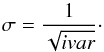 (6)After normalizing ivar with respect to the continuum as described above, the extracted signal-to-continuum spectra are divided by 3σ in order to normalize the noise to values between − 1 and 1. Those are called normalized S/N spectra (NSN-spectra hereafter). As a consequence, the contrast between real signals and noise is increased further and artifacts stemming from a bad sky subtraction or bad pixel are heavily suppressed.
3.4. Feature extraction
To extract the feature vectors, we split the spectra into positive and negative flux components with respect to the fitted continuum (see bottom plot in Fig. 2). We thereby create two feature vectors per spectrum. This simplification allows keeping the entire redshift-dependent information while no longer being dependent on the continuum shape. The separation enables us to compute individual redshifts for absorption and emission. By extracting subregions of this feature vector, we can even obtain redshift information on single spectral regions. All values above the continuum (>0) are included in the feature vector for emission, and all values below the continuum are simply set to zero. For absorption values larger than zero are set to zero. Those extracted vectors are the input for our kNN-search described in Eq. (3).
4. Experiments
We conducted two experiments with different selections of features and different reference samples. In the following they are named Experiment 1 and 2.
4.1. Description of experiments
Both runs have been done on the full set of NSN spectra. For the first experiment, we applied the algorithm to the entire spectra and only distinguish between absorption and emission. In the second experiment we limited the dimensionality of the feature vector by just comparing specific spectral regions where features are expected for the redshift given by SDSS.
Naively, one would expect high precision in the former method because the full information content is available and thus the confusion between features of different origin (e.g., misidentifying Hβ as Hα) should be fairly low. Other emission/absorption signatures are available to cross-validate the redshift and hence minimize the probability of confusion. On the other hand the obtained final regression value is only valid for the entire spectrum and thus generalizes the information content too heavily.
Regions considered.
For this reason a second experiment was conducted with a comparison restricted to single regions where prominent emission/absorption signatures are expected. It is worth noting that this experiment is tailored to detect shifts in individual spectral lines. Additionally, the methodology can be easily extended to allow a clustering or classification of the individual lines. We assume that the redshift of SDSS is correct for the entire spectrum, but we search for redshift deviations in individual components. Since confusion will have a significant impact on the determination of the redshift, we restrict the redshift deviation of the reference sample to a spectral window W defined by  (7)with
 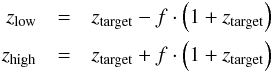 (8)where f is the allowed deviation from the SDSS redshift (ztarget) in units of the speed of light. A list of the spectral regions that have been considered can be found in Table 2. This list contains lines that are usually strong in star-forming and star-bursting galaxies and QSOs. The free parameter f influences the computational efforts, the chance of confusion (improving for small f) and the sensitivity to outliers where huge redshift deviations were achieved with large f, respectively. Throughout this paper, we use a value of f = 0.05. The big disadvantage of the second experiment is that confusion becomes a major concern. Especially for the entire data set, it might be wise not to compare spectra to spectra of any redshift since it is likely that, for example, the Hβ (λ4861) line can look similar to the [OIII] (λ5007) line, see Fig. 3, which obviously would lead to an incorrect regression value. The benefit of this concept is its huge flexibility. Redshifts can now be computed for individual regions independently, so that shifts can be detected. A more detailed discussion of the trade-off of confusion and multiregion regression value determination is given in Sect. 5.
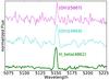 |
Fig. 3 Cut-out of the same spectral region for three spectra with different redshifts. If only this part is available, the Hβ line is indistinguishable from any of the two [OIII] lines. |
4.2. Maximum deviation limit
One of the prerequisites in using the kNN approach was that a clear separation between noise and signal can be made. In principle there are two ways to reject spectra with no signal, the pre- and the post-selection. To preselect one assumes that a signal has a certain shape and exceeds a given S/N limit. This can be simplified further to a measure that compares the average of a spectral region with a nominal value. Because this preselection requires detailed knowledge about the shape, size and symmetry of spectral features, physical knowledge about the morphology of lines is required. To be independent of physical assumptions3, the possibility of a post-selection is chosen. The selected concept assumes that the deviation of the redshifts of the nearest neighbors over all targets follows a smooth distribution. For this distribution an upper limit can be (freely) selected that separates redshift estimates into good and noisy ones. This maximum deviation limit will be abbreviated by MDL.
An even bigger advantage of this method is that it allows experimenting with this free parameter in the evaluation stage, such that the kNN search is not performed for every individual value of MDL.
4.3. Validation strategy
To avoid biases in the regression values and when tuning the parameters, the leave-one-out strategy is used. This means that the closest object (which is always the object itself) is not used for determining the redshift.
The fundamental assumption that most SDSS redshifts are correct has already been discussed in Sect. 3.2. Assuming now that all redshifts are correct, we can compute something like a completeness, a correctness, and a sensitivity. The completeness is a very straightforward measure. It is the fraction of objects for which a redshift could be determined within the respective acceptance limit. In contrast to that the correctness is the fraction of objects where the computed and the SDSS redshift agree within their errors. Finally, the sensitivity gives the reliability of all redshifts; i.e., it gives the typical deviation from the redshift, therefore the standard deviation of the difference between SDSS and computed redshift of all valid spectral features is computed.
4.4. Parameter tuning
Despite the parameters described in the preprocessing step only two parameters have to be fine-tuned for the regression step4. Those are the number of k nearest neighbors used for the comparison and the MDL that marks a spectrum as reliable. With the test strategy described in the previous section, this fine-tuning can be solved on a discrete grid (see Fig. 4). Two separate things are shown in this plot, the large scale behavior of the properties on the righthand side and on the left a zoom-in to the lowest values of the MDL.
With increasing MDL, which is equal to accepting more noisy spectral features, the properties behave just as expected; while the completeness is increasing, the sensitivity and correctness of the model are decreasing. One can further see that the completeness is a fairly flat function up to an MDL of 0.08 where it starts a more rapid, step-wise increase. The regression model breaks already down at a MDL of 0.05 where the sensitivity and correctness show a steep decrease. Since the increase of the completeness is only very tiny for high values of MDL, we now focus on the region of very tiny values of MDL.
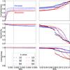 |
Fig. 4 Normalized completeness, sensitivity, and correctness tested against different values of k and MDL. MDL is chosen to be 0.0015 as marked. |
On the small scale, the completeness strongly depends on the choice of the MDL and slight increases in the MDL yield a strong increase in completeness. Then the behavior becomes very flat, so the gain by further increasing the MDL is only marginal. When increasing the MDL 5 times, the completeness fraction increases by less than 2%. It is worth noting that the completeness depends quite heavily on k. Smaller k values result in a more complete regression model. This indicates that the number of good references is in the range of 10−20. For higher values of k more deviation is introduced in the regression model.
The sensitivity of the regression model only decreases in the beginning and then follows a fairly flat behavior with a slightly decreasing tendency. The dependence on the number of used neighbors is only marginal, though one can see that emission favors low k (little number of reference objects), while the sensitivity of the redshift in absorption is slightly better for higher values of k. In the end the fraction of outliers on the good regression side only slightly changes with increasing MDL and k. The decrease over the entire tested range is on the order of 0.5%.
The flat increase in completeness for MDL values greater than 0.001 allows us to minimize the effects on the sensitivity and correctness. We analyzed the impact of the choice of k on the different testing properties as well. The behavior of those with a fixed value of MDL of ≈ 0.0015 can be seen in Fig. 5. An increasing number of nearest neighbors improves the sensitivity at the cost of a lower completeness. Thus as for the MDL, the choice of k depends strongly on the desired completeness and precision.
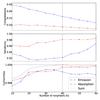 |
Fig. 5 Dependence of test properties on k. For this plot, MDL is fixed to 0.0015. k is chosen to be 40 as marked. |
4.5. Computational efforts
Applying the method described above to the test set is already quite time-consuming on a single machine. It is evident that the computational effort for three million spectra is many times greater than with 16 000; i.e., the time complexity of a brute force kNN search scales with O(n2), thus the calculation time would already be years on a single machine. For future surveys, this number will increase even faster such that more efficient approaches have to be found to resolve that problem. To speed up the calculation we parallelized the computation of the distances. The results presented here should only give an overview of what is possible with even the simplest methods when such a huge data amount is available.
It is worth noting that an online nearest neighbor search of incoming data (streaming) with a spectral database of the size of SDSS (≈3 000 000 spectra) is computationally feasible on a modern laptop. Assuming that a new instrument (e.g., 4MOST, de Jong et al. 2012) will obtain 2400 spectra simultaneously, the approximate comparison time is on the order of 40 h/core using a standard Python implementation. Using a machine with a simple GPU and a C-implementation will yield a speed-up of at least 100 compared to the single-CPU machine and can evaluate such a huge amount of data (<30 min) in less than the typical exposure time. Fortunately, the computation of the distances can be perfectly parallelized, so this method is well suited for larger surveys on modern computer architecture.
As already stated, the computational effort also depends strongly on the number of reference objects used for comparison, and that needs to be tuned carefully in order to minimize computing time. On the other hand, the impact of selection effects is minimized by increasing the number of reference objects that have to be chosen in the most unbiased manner.
5. Results
In the following, we use the median absolut deviation (MAD) as a deviation measure, which is defined as  for a list of values
  . In the following we always use the normalized difference in redshift, which is defined as
 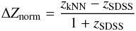 which corresponds to the difference in velcocity in terms of c in the rest frame of the SDSS redshift. In Fig. 4 one can see the behavior of the completeness, sensitivity, and correctness as a function of the MDL as well as for different k. The curves follow the expected behavior; decreasing MDL will yield a low completeness but high-quality redshifts as a result. In the middle is a plateau until the MDL exceeds ≈0.10. Beyond this value the completeness starts to converge to one and the quality of the redshifts to 0, while for the value added catalog a high completeness is desirable with a moderate loss of sensitivity, so MDL = 0.07 and k = 10 are chosen. This increases the fraction of objects with a reliable redshift either in emission or in absorption up to a total of 80%. With this choice of parameters we still have better sensitivity than does SDSS with a significantly lower value in completeness (in SDSS ≈96% of the targets have NO redshift warning). As stated earlier, the choice of the reference sample, especially at high redshifts, will increase this fraction of our method significantly. For example, when we exclude spectra with z> 0.25 the completeness increases to ≈90%.
In the following we concentrate on detecting and verifying outliers using MDL = 0.015 and k = 40. With that choice we have traded high sensitivity for a lower completeness of ≥50%. This enables us to efficiently detect outliers that show wrong or multiple redshift components. In the following, the outlier detection for both experiments is discussed in detail.
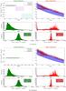 |
Fig. 6 Evaluation of the performance for emission a) and absorption b): the relative deviation from the SDSS redshift as function of the SDSS redshift (top), the distribution of the MAD of the calculated redshift (middle) and the frequency of the relative deviation (bottom) are shown for the good (left) and the rejected noisy (right) spectral features, respectively. The blue background shade in the upper right figure reflects the objects which are entirely dominated by noise and thus their computed redshift just reflects a random draw of redshifts from the initial distribution, see Eq. (9). |
5.1. Experiment 1
When using the entire spectral range for computing the redshift, we can obtain redshifts for 56% (emission) and 49% (absorption) of the spectra. Figure 6 presents the evaluation of the achieved performance. In the second row of each figure, one can see the frequency of deviations for emission and absorption5. As expected, there is an exponential drop-off and an underlying uniform contribution. The top figure shows the relative deviation (in units of the speed of light) between the redshift by SDSS and the computed ones. For nearly all of the objects with prominent features, this deviation is below 0.1%c, which corresponds roughly to the SDSS resolution.
In emission one can see three groups of outliers: three points between a redshift of 0.2 ≤ z ≤ 0.3 (G1, magenta background), a straight line in the lower right of the plot (G2, cyan background), and three points that deviate significantly from the expected redshift below a redshift of z ≤ 0.1 (G3, blue dots). The cause of each of the outliers groups is different but nonetheless understood. The members of G1 are affected by the lack of reference objects in a comparable redshift range (z> 0.2), which agrees perfectly with the distribution shown in Fig. 1. Thus the nearest neighbors will all have a lower redshift, moving all of those points to this region in the plot. It is worth noting that one would naively expect all of those points to lie on a horizontal line, and the deviation from the reference set should be the same for all objects. In fact, it turned out that the lowest point in this group is a truly shifted object. G2 is actually a superposition of the problem just described and what was defined earlier as confusion. This confusion occurs since the relative shift in redshift of ΔZnorm ≈ −0.25 corresponds roughly to the shifts between Hα − Hβ (ΔZnorm = 0.26), Hα − [ OIII ] (ΔZnorm = 0.24), [ NII ] − Hβ (ΔZnorm = 0.26), and [ NII ] − [ OIII ] (ΔZnorm = 0.24). In this case the spectra usually show strong emission in either Hβ or [OIII], which are then (due to missing references) misidentified as [NII] or Hα. Finally spectra with real shifts are likely to be observed close to the horizontal green line. They are discussed further in Sect. 5.3. The behavior of the noisy features can be explained by another superposition of two effects. The first group of objects is the one where the relative deviation is fairly low over the entire redshift range. Those objects are the result of the choice of the MDL – their redshift is still very accurate but they were moved to the uncertain features. A large number of spectra can be described very nicely with the applied model. This indicates that the MDL was selected quite conservatively. The rest of the data points in this plot do not show any signal of an emission feature, so they are just a random selection of redshifts from the initial distribution shown in Fig. 1. The distribution of redshifts is approximated fairly well by a Gaussian (mean = 0.14 and standard deviation = 0.10). The functional form (cf. blue background plot in upper row) is  (9)In absorption two outliers could be detected that show some anomalies that are described well by the computed redshift. Even redshifts with high MAD are still fairly reliable, supporting the restrictive limit on the MDL. The precision in absorption is close in value to the emission, one per mil in units of the speed of light. Obviously the chance of confusion is dramatically lower than for the emission, which is the consequence of having fewer potential features. In a regular galaxy only three strong absorption features can typically be observed.
5.2. Experiment 2
In contrast to the first experiment the number of potential nearest neighbors of a specific spectral region now depends strongly on the choice of the redshift bin and additionally on the likelihood of the respective feature appearing in a galaxy spectra. It then becomes inevitable to discuss the chosen regions individually. To still have a good comparison of the redshifts between the different regions, the MDL is set to 0.0015. For the sake of completeness, all the figures comparing the noisy and the good features are presented in the Appendix A. Without restricting the results any further, the number of potential outliers increases drastically owing to the problem of additional confusion with different spectral features as well as to the limited number of used reference objects. Thus in order to remain clear and minimize the effect of methodological artifacts, the deviation/outlier constraint is not just tested for k = 40 but for a full list of nearest neighbors, namely k = [ 5, 10, 20, 30 ]. If the MAD violates the MDL or if the computed redshift agrees in its tolerance with the SDSS redshift for any k, the object is not marked as an outlier. Likewise, objects that have redshifts z< 0.05 or z> 0.3 are automatically excluded from the outlier detection algorithm because here the limited number of comparison objects introduces spurious redshifts. Since the different regions are biased by different effects, they are discussed in more detail.
In the following we discuss the individual spectral emission and absorption features, along with groups and individual outlying spectra. Exemplarily extensive plots for two spectral features are shown in Figs. A.1 and A.2 for Hβ and NaD, respectively.
5.2.1. Emission
MgII, NeV (λ2, 799, λ3, 346-3,426).
For those spectral regions a redshift of z = 0.45/0.18 is required to allow for a redshift determination. Since the number density of objects is fairly sparse for such high redshifts, and the NeV feature does not occur in many of those spectra, none of the redshifts can be trusted.
[OII] (λ3, 727-3, 729).
This feature does not occur in all star-forming or active galaxies so that fewer than half of the redshifts could be trusted. Even in this small fraction of objects, two outliers were detected that both show an actually shifted [OII]-line that is correctly described by the value determined by us.
Hϵ, Hζ (λ3, 798-3, 835).
One of the objects found to have a shift in the [OII]-feature could be rediscovered. Both the other additional spectral features are real.
Hδ (λ4,102).
This spectral feature only appears in emission for star-forming, bursting and active galaxies. The number of reference objects exhibiting a clear sign of emission is fairly rare. In the corresponding plot one can see that two straight regions are apparent at ΔZnorm = 0.04 / −0.04, which are caused by confusion. The remaining object shows some very strong noise in the vicinity of the expected spectral feature.
Hγ,[OIII] (λ4,342−4,363).
The only two remaining spectra have ΔZnorm = −0.032. When investigating the origin of this shift, it appears that the shift is dominated by noise because the number of active and starburst objects (objects that possibly emit strong Balmer lines) in the specific redshift bins is very low (<5). When selecting the redshift those few objects are therefore strongly dominated by noise. Consequently, this feature is not very reliable as long as no representative reference sample can be selected.
Hβ, [OIII] (λ4, 861-5, 007).
In this spectral region the impact of confusion becomes dominant. Fourteen objects show a reasonably low deviation to be marked as good estimates. The horizontal line at ΔZnorm = 0.03 is caused by a misidentification of the red [OIII] line with the Hβ-feature. The line at ΔZnorm = 0.01 is due to the confusion between the red and the blue [OIII] lines. The negative confusion at ΔZnorm = −0.03 is the reverse effect of the first one. Another horizontal component at ΔZnorm = −0.055 is caused by a misidentification between the blue [OIII] line and HeII emission at λ4,685.
Apart from all this confusion there is one regular shift that cannot be confirmed owing to the lack of other emission features. The MAD for this object (0.0014) is close to the MDL so a lower choice of the MDL would tag this object as unreliable.
Hα, [NII] (λ6, 550-6, 584).
The outlier on the very top of the plot was already marked by the first run and is a truly shifted spectral feature. One of the shifts of the remaining two outliers is the result of an Hα-line in absorption and emission such that the red [NII]-line was mistaken for it. In the other a very weak [NII] emission line led to confusion with the Hα line.
[SII] (λ6, 716-6, 731).
The only object marked in the plot was also detected in the Hα-line as an outlier. It was already marked as an outlier in Experiment 1.
5.2.2. Absorption
CaII (HK) (λ3, 934-3, 969).
All three targets highlighted as outlier are truly shifted spectral features, where one of them is the object already detected in emission (cf. Experiment 1).
Mgb (λ5, 173).
Six of the objects are located on a horizontal line around ΔZnorm = −0.06. This corresponds to a misidentification of the Mgb absorption with the Hβ in absorption. Indeed, all highlighted objects show a very prominent Hβ feature in absorption. Two of the remaining objects have a very strong absorption feature stemming from deficient nightsky subtraction that was not properly described by ivar. Three objects are active galaxies, and they show extremely strong emission features in this region. The number of active galaxies in the reference sample is not sufficient to reproduce this behavior. The remaining object shows a true shift in the Mgb line.
NaD (λ5, 890-5, 896).
For seven spectra a shift of the NaD could be confirmed by a manual inspection. For all the others a badly subtracted sky at around λ7200 was not described correctly by ivar, leading to a very prominent absorption feature that was mistaken for NaD.
5.3. Manually investigated objects
To validate the method, a manual inspection of the outliers is mandatory. A spectrum was investigated if it was selected as an outlier in any of the spectral regions (from Experiments 1 and 2) and if it was not part of one of the horizontal lines introduced by confusion. The outliers have different origins that can be roughly classified into three groups: objects with real multiple redshift components (true), objects with detectoror nightsky artifacts that were not properly described by ivar (fake), and objects where the redshift computation simply failed (wrong).
Thirty-seven objects were eventually investigated manually, three of which have been marked by several features as outliers. Fourteen of the outliers (38%) are spectra with truly shifted redshift components. In 11 of those, the shift between the redshift components is lower than 10 000 km s-1, so those components certainly do have a physical origin. The three remaining spectra of the true class are likely to be superpositions and/or lensed objects. The fake category contains ten objects where a badly described detector/nightsky artifact was confused with NaD or Mgb absorption. It is impossible to exclude those objects previously because there is no unique position or indication of the existence of such a feature. The thirteen spectra in the wrong class are mainly the result of a biased reference sample that also contains a low number of active and star-bursting galaxies. There is a good chance that the fraction of those objects can be significantly decreased if a more representative reference sample is used for the comparison.
A short summary of all manually investigated objects with identifier, SDSS, and computed redshift can be found in Table A.1.
5.4. Most prominent outliers
The most prominent outliers are briefly described here to emphasize the power of this outlier detection scheme. In Fig. 7 one can see the three truly shifted objects with the highest velocity offset. While the first two (J094419.05-004051.44, J120419.07-001855.93) were even tagged independently by the separate runs, the last one (J113154.29+001719.02) did not show up in the second experiment because the relative shift between our computed and the SDSS redshift (0.077c) exceeds the allowed range of the shift (0.060c). In the first and last objects the model applied by SDSS describes the absorption behavior quite well, but the emission features are not described at all such that a second component with a strongly shifted redshift is needed to describe them. While they demonstrate the power of the method quite nicely these objects are astronomically less interesting. Owing to missing signs of interaction, it is likely that they are just simple superpositions of objects. In the i-band of the first object, a tiny and asymmetric arc (cf. Fig. 8) can be seen that could indicate a lensed object.
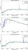 |
Fig. 7 Three most extreme outliers obtained from our regression model. The green line in the background is the SDSS spectrum with the gray spectrum at the bottom being the typical noise deviation. The red curve shows the fitted spectrum with a redshift as obtained by SDSS, the blue curve is the overplotted spectrum with the redshift as obtained by our regression model. |
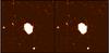 |
Fig. 8 SDSS i-band image of J094419.05-004051.44 (smoothed with Gaussian blur of 3-pixel width). In the right image the asymmetric arc has been overplotted by a green circle. |
The redshift of the second object was estimated incorrectly by SDSS because apparently none of the template models was able to describe both the continuum and the line behavior at the same time. The newly estimated redshift, on the other hand, describes the spectrum quite well. While the new fit does not support the existence of another component, it is worth noting that on the SDSS image a clear symmetric arc can be seen at a distance of a few arcseconds.
5.5. Summary of outliers
In Table A.1 all outliers found are summarized. Targets where a true feature exists are marked. The possible origins for the existence of multiple redshift components are miscellaneous. For a very high shift between the redshifts, the most likely explanation is a chance superposition of two objects. In this case an arc due to gravitational lensing might be observed. The number of gravitational lenses in the near universe is very limited so far (Muñoz et al. 1998). Spectra with the velocity shifts between the lines lower than < 10 000 km s-1 might be good candidates for being super-massive black hole binaries (SMBHB, Tsalmantza et al. 2011; Fu et al. 2012; Popović 2012). The kinematics of the broad line region are a very common cause of such observed line shifts as well (Shen et al. 2011).
Eventually one could only distinguish between the different origins by either deep-imaging (lenses) or follow-up spectroscopy (SMBHB, Liu et al. 2014). High-resolution imaging in the multiple wavelengths could also distinguish single from multiple sources (e.g., Rodriguez et al. 2009).
6. Summary
This paper presents a new methodology that performs a redshift computation based on pre-exisiting SDSS redshifts. The aim is to obtain improved redshifts for emission and absorption, as well as for individual spectral features. This enables astronomers to detect spectra with multiple redshift components. The basic principle of the presented method is to perform a self-consistency check such that objects that look similar should have a comparable redshift.
First of all, it is worth noting that this method performs quite well in calculating the redshift for very different kinds of spectra. The only requirement is that the density of reference objects is reasonably high in the d-dimensional Euclidean space populated by the spectra. It could be shown that with its current set of reference spectra (which is limited to redshifts z ≤ 0.5, but the reference sample is just densely populated until z ≈ 0.2) this method can reach higher sensitivity than the SDSS pipeline for individual spectra. So far, only the completeness is considerably lower than in the SDSS pipeline, but this will be improved using a larger and more representative reference sample that covers all redshifts.
To show the power of this new tool, we presented outliers found in the data set. For this a more conservative (more sensitive, but less complete) parameter set was chosen. We were able to detect outliers by two different statistical redshifts. The first approach focuses on the overall behavior of the spectra, so is less affected by confusion but is less informative. The second approach focuses on the behavior of predefined regions. Its completeness rate is higher; i.e., more objects with exotic behavior have been found. On the other hand, the number of highlighted objects that appear due to methodological artifacts is also increased. In summary both methods yield very interesting objects where the SDSS redshift was incorrect.
Even though these methods work quite well, plenty of parameters exist that are tunable and that have an impact on the final result. In the data preprocessing several models describing the continuum behavior were investigated. The normalization of the spectra with respect to this continuum and their noise might have an effect on the number of true outliers, too. In addition, the feature extraction has a strong impact on the final results and might be tailored to certain scientific needs.
In a next step, we will investigate the impact of the choice of the reference sample. Each redshift bin should contain enough reference objects to minimize systematic effects of to the sample bias. This discussion is part of a forthcoming paper, where the methodology is applied to the full SDSS spectroscopic database.
In a final step, the impact of the mathematical composition of the regression values used in Eq. (3) could be investigated. It would also be interesting to study the behavior of different selection measures, such that a clearer distinction between noisy and good features can be made. Additionally, one could apply a pre- instead of a post-selection to distinguish between signals and noise on the data level. This would make the reduction of the reference sample in the computational step easier, as only reference objects with an existing signal would be used for comparison. On the other hand, it would introduce more biases that have to be tuned by the increased number of parameters. Some physical knowledge about the type of signal that is expected would be required.
Finally, the outlier detection could be modified. Depending on the scientific use case, the trade-off between completeness and sensitivity can be adjusted by using different detection criteria. Those detected outliers can be related to future outlier catalogs. Since we are currently only investigating a small fraction of the database (<1%), a huge number of objects are expected to be marked as outliers for the entire dataset; i.e., that the number of objects to be investigated will be so large (≈5000) that a manual inspection will be extremely time-consuming. At any rate, the discovery potential of this straightforward redshift determination approach is huge. The applicability on new incoming data was already shown on this simplified and just partially representative sub-sample.
This statement is not only valid for the in-sample method presented here but also for the application on other datasets, as long as the wavelength coverage and the target selection criteria are comparable. This is because the data complexity of the reference sample, SDSS in this case, remains the same and thus a comparable number of references is needed for similiar precision.
Acknowledgments
Funding for SDSS-III has been provided by the Alfred P. Sloan Foundation, the Participating Institutions, the National Science Foundation, and the US Department of Energy Office of Science. The SDSS-III web site is http://www.sdss3.org/. SDSS-III is managed by the Astrophysical Research Consortium for the Participating Institutions of the SDSS-III Collaboration including the University of Arizona, the Brazilian Participation Group, Brookhaven National Laboratory, Carnegie Mellon University, University of Florida, the French Participation Group, the German Participation Group, Harvard University, the Instituto de Astrofisica de Canarias, the Michigan State/Notre Dame/JINA Participation Group, Johns Hopkins University, Lawrence Berkeley National Laboratory, Max Planck Institute for Astrophysics, Max Planck Institute for Extraterrestrial Physics, New Mexico State University, New York University, Ohio State University, Pennsylvania State University, University of Portsmouth, Princeton University, the Spanish Participation Group, University of Tokyo, University of Utah, Vanderbilt University, University of Virginia, University of Washington, and Yale University. The authors thank Michael Schick for very fruitful discussions on the topic of uncertainty quantification. S.D.K. would like to thank the Klaus Tschira Foundation for their financial support.
References
- Ahn, C. P., Alexandroff, R., Allen de Prieto, C., et al. 2014, ApJS, 211, 17 [NASA ADS] [CrossRef] [Google Scholar]
- Ball, N. M., & Brunner, R. J. 2010, Int. J. Mod. Phys. D, 19, 1049 [NASA ADS] [CrossRef] [Google Scholar]
- Bellman, R., & Bellman, R. E. 1961, Adaptive Control Processes: A Guided Tour (Princeton University Press) [Google Scholar]
- Bolton, A. S., Burles, S., Schlegel, D. J., Eisenstein, D. J., & Brinkmann, J. 2004, AJ, 127, 1860 [NASA ADS] [CrossRef] [Google Scholar]
- Bolton, A. S., Schlegel, D. J., Aubourg, É., et al. 2012, AJ, 144, 144 [NASA ADS] [CrossRef] [Google Scholar]
- Borne, K. 2009, ArXiv e-prints [arXiv:0911.0505] [Google Scholar]
- Cui, X.-Q., Zhao, Y.-H., Chu, Y.-Q., et al. 2012, RA&A, 12, 1197 [Google Scholar]
- de Jong, R. S., Bellido-Tirado, O., Chiappini, C., et al. 2012, in SPIE Conf. Ser., 8446 [Google Scholar]
- Eisenstein, D. J., Annis, J., Gunn, J. E., et al. 2001, AJ, 122, 2267 [NASA ADS] [CrossRef] [Google Scholar]
- Fu, H., Yan, L., Myers, A. D., et al. 2012, ApJ, 745, 67 [Google Scholar]
- Gieseke, F. 2011, dissertation, Universität Oldenburg [Google Scholar]
- Gieseke, F., Polsterer, K. L., Thom, A., et al. 2011, ArXiv e-prints [arXiv:1108.4696] [Google Scholar]
- Hastie, T., Tibshirani, R., & Friedman, J. 2009, The Elements of Statistical Learning: Data Mining, Inference, and Prediction., 2nd edn. (Springer) [Google Scholar]
- Laurino, O., D’Abrusco, R., Longo, G., & Riccio, G. 2011, MNRAS, 418, 2165 [NASA ADS] [CrossRef] [Google Scholar]
- Liu, X., Shen, Y., Bian, F., Loeb, A., & Tremaine, S. 2014, ApJ, 789, 140 [NASA ADS] [CrossRef] [Google Scholar]
- Meusinger, H., Schalldach, P., Scholz, R.-D., et al. 2012, A&A, 541, A77 [NASA ADS] [CrossRef] [EDP Sciences] [Google Scholar]
- Muñoz, J. A., Falco, E. E., Kochanek, C. S., et al. 1998, Ap&SS, 263, 51 [NASA ADS] [CrossRef] [Google Scholar]
- Polsterer, K. L., Zinn, P.-C., & Gieseke, F. 2013, MNRAS, 428, 226 [NASA ADS] [CrossRef] [Google Scholar]
- Popović, L. Č. 2012, New Astron. Rev., 56, 74 [Google Scholar]
- Richards, G. T., Fan, X., Newberg, H. J., et al. 2002, AJ, 123, 2945 [NASA ADS] [CrossRef] [Google Scholar]
- Richards, J. W., Freeman, P. E., Lee, A. B., & Schafer, C. M. 2009, ApJ, 691, 32 [NASA ADS] [CrossRef] [Google Scholar]
- Rodriguez, C., Taylor, G. B., Zavala, R. T., Pihlström, Y. M., & Peck, A. B. 2009, ApJ, 697, 37 [NASA ADS] [CrossRef] [Google Scholar]
- Shen, Y., Richards, G. T., Strauss, M. A., et al. 2011, ApJS, 194, 45 [NASA ADS] [CrossRef] [Google Scholar]
- Strauss, M. A., Weinberg, D. H., Lupton, R. H., et al. 2002, AJ, 124, 1810 [NASA ADS] [CrossRef] [Google Scholar]
- Tsalmantza, P., Decarli, R., Dotti, M., & Hogg, D. W. 2011, ApJ, 738, 20 [Google Scholar]
- York, D. G., Adelman, J., Anderson, Jr., J. E., et al. 2000, AJ, 120, 1579 [Google Scholar]
Appendix A: Appendix A
Summary of all manually investigated spectra.
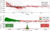 |
Fig. A.1 Analysis of the Hβ,[OIII] region. One can see the relative difference in redshift against the SDSS redshift (top), the distribution of the deviations (middle), and a histogram of the relative difference in redshift (bottom). Noisy spectral features are marked in red, good features in green. |
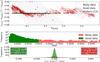 |
Fig. A.2 Analysis of the NaD region. One can see the relative difference in redshift against the SDSS redshift (top), the distribution of the deviations (middle), and a histogram of the relative difference in redshift (bottom). Noisy spectral features are marked in red, good features in green. |
All Tables
Parameters used in preprocessing with tested value range and impact on the outcoming distribution as well as on the time effort for the preprocessing.
All Figures
|
Fig. 1 Comparison of the redshift distribution of the selected subsample (green) and the entire SDSS (blue). There is a steep drop in the frequency toward redshifts z> 0.25. Single redshift bins are apparently undersampled. |
| In the text | |
|
Fig. 2 Top: spectrum with uncertainty. Upper center: decomposed continuum representation by Gaussians. Lower center: spectrum with continuum fit and masked regions (ignored when fitting the continuum). Bottom: the extracted feature vectors are solely all pixel values with a value above (below) zero for emission (absorption), and all other values are set to zero. |
| In the text | |
|
Fig. 3 Cut-out of the same spectral region for three spectra with different redshifts. If only this part is available, the Hβ line is indistinguishable from any of the two [OIII] lines. |
| In the text | |
|
Fig. 4 Normalized completeness, sensitivity, and correctness tested against different values of k and MDL. MDL is chosen to be 0.0015 as marked. |
| In the text | |
|
Fig. 5 Dependence of test properties on k. For this plot, MDL is fixed to 0.0015. k is chosen to be 40 as marked. |
| In the text | |
|
Fig. 6 Evaluation of the performance for emission a) and absorption b): the relative deviation from the SDSS redshift as function of the SDSS redshift (top), the distribution of the MAD of the calculated redshift (middle) and the frequency of the relative deviation (bottom) are shown for the good (left) and the rejected noisy (right) spectral features, respectively. The blue background shade in the upper right figure reflects the objects which are entirely dominated by noise and thus their computed redshift just reflects a random draw of redshifts from the initial distribution, see Eq. (9). |
| In the text | |
|
Fig. 7 Three most extreme outliers obtained from our regression model. The green line in the background is the SDSS spectrum with the gray spectrum at the bottom being the typical noise deviation. The red curve shows the fitted spectrum with a redshift as obtained by SDSS, the blue curve is the overplotted spectrum with the redshift as obtained by our regression model. |
| In the text | |
|
Fig. 8 SDSS i-band image of J094419.05-004051.44 (smoothed with Gaussian blur of 3-pixel width). In the right image the asymmetric arc has been overplotted by a green circle. |
| In the text | |
|
Fig. A.1 Analysis of the Hβ,[OIII] region. One can see the relative difference in redshift against the SDSS redshift (top), the distribution of the deviations (middle), and a histogram of the relative difference in redshift (bottom). Noisy spectral features are marked in red, good features in green. |
| In the text | |
|
Fig. A.2 Analysis of the NaD region. One can see the relative difference in redshift against the SDSS redshift (top), the distribution of the deviations (middle), and a histogram of the relative difference in redshift (bottom). Noisy spectral features are marked in red, good features in green. |
| In the text | |
Current usage metrics show cumulative count of Article Views (full-text article views including HTML views, PDF and ePub downloads, according to the available data) and Abstracts Views on Vision4Press platform.
Data correspond to usage on the plateform after 2015. The current usage metrics is available 48-96 hours after online publication and is updated daily on week days.
Initial download of the metrics may take a while.