| Issue |
A&A
Volume 576, April 2015
|
|
|---|---|---|
| Article Number | A95 | |
| Number of page(s) | 13 | |
| Section | Interstellar and circumstellar matter | |
| DOI | https://doi.org/10.1051/0004-6361/201424556 | |
| Published online | 08 April 2015 | |
Mutual influence of supernovae and molecular clouds⋆
1 Laboratoire AIM, Paris-Saclay, CEA/IRFU/SAp – CNRS – Université Paris Diderot, 91191 Gif-sur-Yvette Cedex, France
e-mail: This email address is being protected from spambots. You need JavaScript enabled to view it.
2 LERMA (UMR CNRS 8112), École Normale Supérieure, 75231 Paris Cedex, France
Received: 8 July 2014
Accepted: 29 October 2014
Abstract
Context. Molecular clouds are known to be turbulent and strongly affected by stellar feedback. Moreover, stellar feedback is believed to drive turbulence at large scales in galaxies.
Aims. We study the role played by supernovae in molecular clouds and the influence of the magnetic field on this process.
Methods. We performed three-dimensional numerical simulations of supernova explosions, in and near turbulent self-gravitating molecular clouds. In order to study the influence of the magnetic field, we performed both hydrodynamical and magnetohydrodynamical simulations. We also ran a series of simple uniform density medium simulations and developed a simple analytical model.
Results. We find that the total amount of momentum that is delivered during supernova explosions typically varies by a factor of about 2, even when the gas density changes by 3 orders of magnitude. However, the amount of momentum delivered to the dense gas varies by almost a factor of 10 if the supernova explodes within or outside the molecular cloud. The magnetic field has little influence on the total amount of momentum injected by the supernova explosions but increases the momentum injected into the dense gas.
Conclusions. Supernovae that explode inside molecular clouds remove a significant fraction of the cloud mass. Supernovae that explode outside have a limited influence on the cloud but nevertheless remove a substantial amount of gas at densities between 1 cm-3 and 100 cm-3, that would be forming stars later. It is thus essential to know sufficiently well the correlation between supernovae and the surrounding dense material in order to know whether supernovae can regulate star formation effectively.
Key words: ISM: clouds / ISM: magnetic fields / ISM: structure / ISM: supernova remnants / turbulence / stars: formation
Appendices are available in electronic form at http://www.aanda.org
© ESO, 2015
1. Introduction
Understanding what regulates star formation within galaxies remains an unsolved problem. While it seems clear that it is a consequence of fundamental processes such as gravity, turbulence, and magnetic field, it has become clear that stellar feedback plays a major role both in limiting the star formation efficiency within actively star forming clouds and in triggering large-scale interstellar turbulence. In turn, turbulence together with gravity contribute to regulating the generation of star forming molecular clouds.
Among other processes such as ionising radiation (e.g., Matzner 2002), stellar outflows, or stellar winds, supernovae (Mac Low & Klessen 2004) are thought to play a fundamental role because they contain a very significant amount of energy and momentum. Many studies that have attempted to simulate a galactic disk have included supernova feedback both at the scale of a whole galaxy (e.g., Tasker & Bryan 2006; Dubois & Teyssier 2008; Bournaud et al. 2010; Kim et al. 2011; Dobbs et al. 2011; Tasker 2011; Hopkins et al. 2011; Renaud et al. 2013), and at the kpc scale (Slyz et al. 2005; Avillez & Breitschwerdt 2005; Joung & Mac Low 2006; Hill et al. 2012; Kim et al. 2011, 2013; Gent et al. 2013; Hennebelle & Iffrig 2014). In these models it is typically found that the supernova feedback can efficiently trigger large-scale turbulence in the interstellar medium (ISM) leading to a velocity dispersion on the order of 6−8 km s-1. It is also found that supernovae can prevent runaway collapse, leading to star formation rates that are in reasonable agreement with observed values (Kim et al. 2011, 2013; Hennebelle & Iffrig 2014).
To model supernovae in galactic environments, different strategies have been developed. The most fundamental problem is due to the somewhat coarse resolution that is employed in these large-scale studies (going from typically a few tens of parsecs to a few parsecs). It is not possible to follow the supernova explosions with the resolution required to describe them accurately and in particular to compute properly the impact they have on the gas. More precisely, during the Sedov phase (see below for further description), the hot gas that fills the supernova bubble is adiabatic and thermal energy is being converted into kinetic energy as the expansion proceeds. When the cooling time of the dense shell that surrounds the bubble becomes comparable to the dynamical time, the thermal energy is efficiently radiated away and the propagation is driven by the shell momentum which stays nearly constant. Knowing precisely this momentum is important in the context of interstellar turbulence and its replenishment. While some authors have directly deposited thermal energy in few grid cells around the supernova location (e.g., Avillez & Breitschwerdt 2005; Joung & Mac Low 2006; Hill et al. 2012), some others have directly considered the momentum injected (e.g., Kim et al. 2011, 2013) in the gas by inserting a velocity field that is radial and diverging. While the first approach may be more self-consistent, it leads to very small time steps because of the very high temperatures (107−108 K) reached in the simulations. Moreover, it is generally assumed that the supernova remnants are initially spherical at scales comparable to the resolution which is typically a few pc. Whether that is a fair assumption may depend on the exact place where the supernova is exploding.
The way to implant supernova feedback in these simulations is largely based on the specific models that have been developed to study the evolution of supernova remnants in a uniform medium (Oort 1951; Sedov 1959; Chevalier 1974; McKee & Ostriker 1977; Cioffi et al. 1988; Ostriker & McKee 1988; Blondin et al. 1998). Three stages are commonly recognized for the evolution of supernova remnants. The first phase is a free expansion phase, where the initial ejecta simply sweep up the ISM. When the mass swept up by the remnant becomes comparable to the mass of the ejecta, the evolution switches to an adiabatic phase as described by the Sedov-Taylor model (Sedov 1959) where the shell radius evolves with time as Rs ∝ t2/5. This phase lasts until the gas behind the shock cools down efficiently (which typically happens around 106 K), at which point a dense shell forms and snowplows through the ISM thanks to the pressure of the hot gas inside. The snowplow phase has two stages: at the beginning, the evolution is driven by the internal pressure, following the pressure-driven snowplow model (Cioffi et al. 1988). If the ambient medium is dense, this phase can be very short and have a timescale similar to the transition timescale. When the internal pressure support vanishes, the shell expands freely through the medium, following the momentum-conserving snowplow model (Oort 1951) where the shell radius follows Rs ∝ t1/4. To address the question of the efficiency with which supernovae can drive the turbulence into the galaxies, an important question is how much momentum is delivered by supernova remnants in the ISM? In this respect a remarkable result has been inferred (e.g., Blondin et al. 1998): the total momentum injected by the supernova has a weak dependence on the gas density (see below for more details) of the surrounding gas suggesting that a constant value can be assumed in simulations.
Generally speaking, because the ISM is very inhomogeneous, the medium in which supernova remnants propagate is expected to present density contrasts of several orders of magnitude. How does it modify the supernova remnant evolution? Does it affect the total amount of momentum that is eventually delivered in galaxies? Another related aspect that has received little attention is the influence that magnetic fields can have on the remnant, in particular whether the magnetic field can alter the amount of momentum injected into the ISM.
A complementary question is the impact that supernovae can have on molecular clouds as they explode. While the impact of HII regions (Matzner 2002; Dale et al. 2012, 2013), protostellar outflows (Li & Nakamura 2006), and the combined effect of protostellar outflows and stellar winds (Dale et al. 2014) has been investigated, the impact supernovae might have on the molecular clouds has received less attention. It is currently estimated that about 10 − 20% of the observed supernova remnants interact with a molecular cloud (Fukui et al. 2003; Hewitt et al. 2009; Chen et al. 2013; Slane et al. 2014). The significance of this number is, however, not straightforward. While one would expect about 1000 supernova remnants in our Galaxy, only ≃ 300 have been observed so far (e.g., Brogan et al. 2006). The reason for this difference has not been clearly established. On the one hand supernovae that explode in a rarefied medium (n ≪ 1 cm-3) may explode without leaving an identifiable remnant (Chu & Mac Low 1990), but on the other hand, supernovae that explode in a dense medium will have a small remnant radius and will quickly dissipate (see Fig. 2), and thus may also be difficult to see. Therefore the question of where most of the remnants are located remains to be clarified.
Motivated by evidence for interaction between supernovae and molecular clouds such as N49 (Shull 1983), a few analytical studies have been performed (Shull et al. 1985; Chevalier 1999). More recently, hydrodynamical numerical simulations of a supernova explosion taking place in a dense clump have been performed by Rogers & Pittard (2013). These simulations include stellar winds, which operate before supernovae explode. They do not however include gravity and magnetic field. The authors conclude that the supernova remnant tends to escape the cloud quickly without depositing a substantial fraction of its energy. They nevertheless show that the supernovae trigger a mass flux that is about 10 times the loss induced by the stellar winds. A detailed study of the effects of stellar winds, photoionization and supernova explosions in a uniform medium has been done by Geen et al. (2014).
In this paper, we investigate the evolution of supernova remnants in molecular clouds. To quantify accurately the amount of momentum that is delivered in the surrounding medium, we focus on a single event. We perform numerical simulations of supernovae in uniform and turbulent, cloud-like medium, taking into account cooling, self-gravity, and magnetic field. We specifically investigate the role of the last by comparing hydrodynamical and magnetized simulations. To assess our calculations, we present a simple but robust model for momentum and kinetic energy feedback, based on the well-known remnant evolution models (Oort 1951; Sedov 1959) and compare it to our simulations.
Section 2 describes the numerical setup: the physics taken into account, the initial conditions, and the resolution. The results of the uniform medium simulations are detailed in Sect. 3, and the results of the turbulent simulations are described in Sect. 4. Section 5 concludes the paper.
2. Numerical setup
2.1. Physical processes
Our simulations include various physical processes known to be important in molecular clouds. We solve the ideal magnetohydrodynamics (MHD) equations with self-gravity and take into account the cooling and heating processes relevant to the ISM.
The equations we solve are
 with ρ, v, P, B, φ, and E respectively being the density, velocity, pressure, magnetic field, gravitational potential, and total (kinetic plus thermal plus magnetic) energy. The loss function ℒ, includes UV heating and a cooling function with the same low-temperature part as in Audit & Hennebelle (2005) and the high-temperature part based on Sutherland & Dopita (1993), resulting in a function similar to the one used in Joung & Mac Low (2006).
We trigger supernovae at given positions in space and time by injecting 1051 erg of thermal energy within a sphere of radius equal to 2 computing cells.
2.2. Uniform density simulations
As a preliminary study, we run simulations of a supernova remnant going through a uniform medium, in order to compare our results with previous work (Oort 1951; Sedov 1959; Chevalier 1974; Cioffi et al. 1988; Ostriker & McKee 1988). We consider several densities ranging from 1 to 1000 particles per cubic centimeter, with an appropriate box size between 160 pc and 40 pc. The gas is initially at thermal equilibrium. Table 1 gives the four initial conditions.
Initial conditions for the uniform cases.
To study the influence of the magnetic field, we run a set of hydrodynamical simulations and a set of MHD simulations for which the magnetic field is initially uniform and has an intensity of 5 μG. The results of these simulations are similar to the hydrodynamical case and are described in Appendix C.
2.3. Turbulent simulations
Clouds are turbulent and present large density contrasts and a complex structure induced by supersonic turbulence. In order to reproduce this in our simulations, we set up a spherical density profile and we add a turbulent velocity field; we then let the cloud evolve for about one crossing time.
More precisely, we consider a spherical cloud with a profile given by ρ = ρ0/ (1 + (r/r0)2) where ρ0 = 9370 cm-3 and r0 = 1.12 pc. The edge density is initially equal to ρ0/ 10. The total mass within this inner region is 104M⊙. In order to avoid a sharp transition with the diffuse ISM and to mimic the HI haloes observed around molecular clouds (e.g., Elmegreen & Elmegreen 1987; Hennebelle & Falgarone 2012), we add around it a uniform density cloud of density ρ0/ 100 ≃ 93 cm-3. The radius of this HI halo is about 6.8 pc and it contains a mass equal to about 5 × 10³M⊙. In the rest of the computational box the initial density is equal to 1 cm-3. The cloud is initially at thermal equilibrium and is surrounded by warm neutral medium at a temperature of 8000 K.
The ratio of the thermal over gravitational energy is initially equal to about 1%. We inject a turbulent velocity field into the cloud. The velocity field presents a Kolmogorov power spectrum and has random phase. The kinetic energy is initially about 100% of the gravitational energy meaning that the cloud is globally supported by turbulence. We let the cloud evolve for 1.25 Myr in order for the turbulence to develop and trigger density (and magnetic field) fluctuations self-consistently, before adding a supernova.
To explore the influence that the supernova position may have on the result, we run three simulations with three different supernova positions (inside, at the border and outside of the cloud), and one without supernova. Figure 1 shows the positions of the supernova explosions with respect to the cloud. In the inside run, the supernova explodes in a density of about 700 cm-3, in the border run the density is closer to 20 cm-3, and in the outside run it is about 1.2 cm-3.
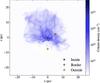 |
Fig. 1 Positions of the supernovae injected in the cloud simulations. |
2.4. Numerical code and resolution
We run our simulations with the RAMSES code (Teyssier 2002; Fromang et al. 2006), an adaptive mesh code using a Godunov scheme and a constrained transport method to solve the MHD equations, therefore ensuring the nullity of the magnetic field divergence. We use two levels of adaptive mesh refinement on a 2563 base grid, leading to a maximum resolution around 0.05 pc for the turbulent case for which the box size is equal to 50 pc, and between 0.04 and 0.16 pc for the uniform case. The refinement criterion is based on the Jeans length, which must be described by at least 10 computational cells in the turbulent cloud runs and on the pressure gradient in the uniform density runs. We limited the resolution because of the presence of very hot (temperatures over 107 K), high-velocity (over 100 km s-1) gas due to the supernova, which enforces a small time step. We integrate until we reach stationarity in the uniform case. In the turbulent cloud runs, since gravity is treated, the cloud keeps evolving and we have integrated up to about 5 Myr which is sufficient to quantify the impact of the supernova on the cloud.
For the turbulent simulations, the blast waves quickly reach the edge of the computational domain and in order to let the energy flow out of the box, we use vanishing gradient boundary conditions, except for the normal component of the magnetic field for which a vanishing divergence condition is enforced.
To assess our results, we have also performed two runs with a base grid of 5123 and two more adaptive mesh refinement levels. One of these runs has the same computational box size of 50 pc, therefore implying a spatial resolution 2 times higher while the other one has a box size equal to 100 pc, which allows us to follow the supernova remnant for a longer time and to verify that the total amount of momentum injected in the surrounding ISM has indeed reached stationarity.
3. Evolution of a supernova remnant in a uniform medium
As recalled previously, three phases are typically expected during supernova explosions, the free expansion phase for which the mass of the remnant dominates the swept-up mass; the Sedov-Taylor phase, during which the expansion is adiabatic; and finally the snowplow phase, during which the dense shell can radiate energy efficiently. In our simulations, given the temporal and spatial resolution, we cannot observe the free expansion phase. We observe the adiabatic phase, the pressure-driven snowplow phase, and the momentum-conserving snowplow phase (for the runs with the highest ambient densities).
3.1. Simple analytical trends
For the adiabatic phase, Sedov’s analytical model (Sedov 1959) predicts a total momentum of  (6)where p43 is the total momentum in units of 1043 g cm s-1, n0 is the particle density in cm-3, E51 is the supernova energy in units of 1051 erg, and t4 is the age of the remnant in units of 104 yr.
We define the transition time ttr as the moment when the age of the remnant becomes equal to the cooling time τcool of the shell which is given by  (7)where ns and Ts are the gas density and temperature of the shell, and Λs the net cooling (in erg cm3 s-1).
Below we estimate the transition time ttr numerically, but it is worth inferring explicitly the relevant dependence. The net cooling Λs can be approximated as (e.g., Blondin et al. 1998)  (8)The temperature and the density in the shell are given by the Rankine-Hugoniot conditions. For a monoatomic gas we thus have
  (9)The evolution of the shell radius is given by Rs ∝ (Et2/n0)1/5. Thus we get
  (10)Combining Eqs. (7)−(10), we get
  (11)therefore
  (12)Using Eqs. (6) and (12), we can estimate the dependence of the shell momentum at the transition time, ttr, and we get
  (13)Thus, we see that the total momentum delivered in the ISM has a weak dependence on the medium density. For example, changing the density by a factor of 103, leads to a momentum variation of about 2 − 2.5.
3.2. Momentum injection: result
Figure 2 shows the integrated radial momentum as a function of time for the four uniform density simulations. We clearly observe two phases of the remnant’s evolution: the adiabatic (Sedov-Taylor) phase, conserving energy for which the momentum follows  , and the momentum-conserving (for the highest ISM densities only), and pressure-driven snowplow (Oort 1951; Cioffi et al. 1988). Figure 2 also shows the analytical prediction stated by Eq. (6)and valid before the transition time. As can be seen the agreement is excellent.
 |
Fig. 2 Integrated radial momentum for the uniform simulations. The thin straight lines correspond to the analytical trends described in Sect. 3.1. Two main phases can be distinguished. First, during the Sedov-Taylor phase the momentum increases with time. Then, during the radiative snowplow phase the momentum is nearly constant. The dependence of the momentum on the ISM density is rather shallow. |
To model analytically the second phase, we solve numerically the equation ttr = τcool; that is to say, we use the complete cooling function instead of using Eq. (8). For the highest ambient densities (n0 ≳ 10), the momentum injection is reasonably well fitted by the momentum-conserving snowplow model with the final momentum pf taken to be the momentum of a Sedov-Taylor blast wave at 2ttr (the numerical values are given in Table 2). Some small deviations are found with the lowest density case because the pressure within the shell is still higher than the surrounding pressure and the shell keeps accelerating. When the surrounding gas density varies by 3 orders of magnitude, the total momentum varies by a factor of about 2.5.
Transition time ttr and final momentum pf as a function of the ambient density n0.
We also compared the injected kinetic energy with analytical trends derived from the same models, again with good agreement. The details are given in Appendix A.
Altogether, the numerical and analytical results agree well with previous works. Importantly, they show that the total amount of momentum delivered in the surrounding ISM is expected to have a weak dependence on the surrounding density.
 |
Fig. 3 Column density maps for the turbulent hydrodynamical simulations. Top panel: no supernova, 0.27,0.85,1.4 Myr after injection time; middle panel: supernova inside; bottom panel: supernova outside, both after 100, 200 and 750 kyr. |
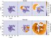 |
Fig. 4 Temperature maps for the turbulent hydrodynamical simulations 1, 20 and 100 kyr after supernova injection time. Top panel: supernova inside; bottom panel: supernova outside (in this view the explosion takes place behind the cloud). |
4. Supernova explosions in turbulent molecular clouds
We now present the simulation results for supernova explosions within molecular clouds. We performed both hydrodynamical and MHD runs. The results of the MHD runs are relatively similar to the hydrodynamical runs and are described in Appendix C. The main difference is that the magnetic field tends to couple the different parts of the cloud, so that supernovae exploding inside have more impact.
4.1. Qualitative description
Figures 3 and 4 show the column density and a temperature slice (z = 0) of the cloud without supernova (top panels), with the supernova inside (middle panels) and outside (bottom panels) (see Fig. 1) at three different time steps. The top panels show a complex multi-scale column density similar to what has been found in many simulations (e.g., Ballesteros-Paredes et al. 2007; Hennebelle & Falgarone 2012). The dense gas rapidly collapses into several objects under the influence of gravity. The second row shows that the hot gas that is initially located inside the dense cloud is rapidly able to escape through channels of more diffuse gas, which has been pushed by the high pressure. Once it reaches the outside medium, a bubble forms and propagates as found previously. The propagation in the rest of the cloud remains limited but happens nevertheless. Indeed, the high pressure enhances the contrast inside the cloud by creating regions of very low density and by compressing further the dense clumps.
The temperature plot (Fig. 4) also reveals interesting behavior. In the inside run, the high pressure gas quickly opens up a chimney through the cloud by pushing the diffuse material. Once it reaches the diffuse ISM, the supernova remnant starts expanding and develops into a spherical shell. The outside run shows a different evolution. The explosion is broadly spherical from the very beginning. The hot gas tends to penetrate in between the dense regions within the cloud and quickly surrounds it, therefore compressing the diffuse material.
4.2. Total momentum injection
In order to quantify the overall impact a supernova embedded in a molecular cloud can have on the surrounding ISM, we first calculate the total radial momentum and kinetic energy as a function of time. Since the gas is initially moving, it may not be straightforward to discriminate between the contribution of the supernova and the initial condition. However, the momentum before the supernova explodes is about 10 times smaller than the peak value reached once the supernova has taken place. Because the results concerning the injection of kinetic energy are of lesser importance, we describe them in Appendix A.
The top panel of Fig. 5 shows the evolution of radial momentum for the three runs, inside, border, and outside, compared to the models described in Sect. 3.2 valid for the uniform density runs. The vertical dashed lines show the time at which the supernova remnant starts leaving the box and at this point, or shortly after, the total momentum decreases. The bottom panel of Fig. 5 shows the results for the same simulation, but performed with a computational box 2 times larger. As can be verified from the total momentum values, the maximum obtained with the 50 pc box is close to the maximum value obtained with the 100 pc box. Numerical convergence can also been assessed from this same diagram as a simulation with 2 times better resolution is also presented.
The injected momentum follows an evolution that is different from any of the uniform density models. This is relatively unsurprising given that the structure of the clouds is far from spherical and entails a wide distribution of densities which spans about 6 orders of magnitude (see Appendix B for details). We note that the trends are qualitatively similar to the uniform density case; that is to say, the outside run tends to be closer to the lower density uniform models than the inside run. In spite of these significant differences with the uniform density runs, the total momentum injected by the supernova does not vary much and remains close to the values inferred in the uniform density case, i.e., a few 1043 g cm s-1.
This result constitutes an important generalization of the uniform models and suggests that the feedback from supernovae in star forming regions and, more generally in galaxies, can be modeled by adopting a simple prescription of a few 1043 g cm s-1 being released in the ISM. Similar results have been found in recent works (Martizzi et al. 2014; Kim & Ostriker 2014).
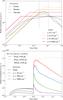 |
Fig. 5 Top panel: total radial momentum, comparison between turbulent simulations and the analytical model for various densities. The vertical lines correspond to the time at which the gas starts leaving the computational domain (from left to right: border, outside, inside). Bottom panel: inside run for two different box sizes and two numerical resolutions. |
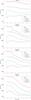 |
Fig. 6 Mass above density thresholds 10,100,1000 cm-3 in the case without supernova (top panel) and outside (second panel), border (third panel) and inside (bottom panel) runs. |
4.3. Mass distributions: impact of the supernova on the cloud
As can be seen in Fig. 6, which shows the mass above various thresholds as a function of time in the four runs (without supernova, outside, border, and inside), the supernova does not change the high-density part of the mass distribution (compared to the rest of the gas), but produces very diffuse gas and hot material. The details of the density distribution, not shown here for conciseness, are presented in Appendix B.
In the run without feedback (top panel), the fraction of gas of densities larger than 10 and 102 cm-3 drops during the first 2 Myr because the cloud is slightly supervirial and therefore expands. As turbulence decays, gravity takes over and the mass of gas denser than 102 and 103 cm-3 increases with time as the collapse proceeds. We note that the decrease of the total mass is due to diffuse gas leaving the computational box. While this leak of material remains limited in the run without supernova, it is more important for the runs with supernova explosions. As shown in the bottom panel of Fig. 5, this effect does not affect the 102 and 103 cm-3 thresholds, and affects the 10 cm-3 threshold only marginally. This can be seen by comparing the solid lines (50 pc box size) with the dotted ones (100 pc box size).
In the inside run (bottom panel of Fig. 6), the amount of gas denser than 102 and 103 cm-3 drops sharply after the supernova explosions and after 2 Myr reaches values of about 6 and 7 × 10³M⊙, respectively. Later evolution suggests that these numbers do not evolve significantly. At 4 − 5 Myr, these masses are almost 2 times smaller than in the run without supernova. This clearly shows the impact that supernova feedback has on molecular clouds. For the case of the present configuration, that is to say a cloud of mass ≃ 104M⊙ which is about 2 times supervirial, a supernova can reduce the mass that would eventually form stars by a factor of about 2 (see Sect. 4.5 for a more quantitative estimate).
As can be seen from the outside and border runs (second and third panels, respectively), this effect is very sensitive to the position of the supernova in the cloud. The amount of dense gas is only slightly reduced in the outside run with respect to the run without supernova. This is in good agreement with the results inferred by Hennebelle & Iffrig (2014) where kpc simulations were performed. In particular, they found that the impact that supernovae have in reducing the star formation rate decreases as the distance between the supernova and the collapsing regions (represented by Lagrangian sink particles) increases.
4.4. Momentum injection with respect to density
Figure 7 shows the injected radial momentum for three density thresholds and the three supernova locations. Significantly less momentum is injected in denser regions. For the inside runs and for the 102 and 103 cm-3 density thresholds, the amount of momentum is about 1.2 and 0.7 × 1043 g cm s-1 respectively; these values are about 0.3 and 0.1 × 1043 g cm s-1 for the outside runs.
 |
Fig. 7 Evolution of momentum for densities above thresholds 10,100, and 1000 cm-3 in the outside, border, and inside cases. |
In the case when the supernova explosion takes place inside the cloud, momentum is transferred to high-density medium more efficiently than in the other cases, probably because the supernova remnant is trapped within the dense gas of the cloud, whereas in the other cases a significant part of the remnant moves through diffuse medium. The momentum associated with dense gas quickly drops because this dense high momentum gas quickly reexpands and therefore becomes diffuse, in good agreement with the bottom panel of Fig. 6.
This shows once again that the impact supernovae have on the cloud significantly depends on their positions. While the differences between the inside and outside runs show that a shift of a few pc in distance can make a significant difference to the impact a supernova can have on the clouds, supernovae exploding even farther away from the clouds would obviously have an even weaker impact on the dense gas. This highlights the fact that while the amount of momentum injected into the ISM is a very useful piece of information, it is nevertheless vastly insufficient. A more detailed knowledge of exactly where a supernova occurs is necessary in order to quantify the real influence it has on the ISM.
4.5. An analytical estimate
To estimate the fraction of mass, fm that is expelled by the supernova explosion, we can simply compare the amount of momentum that is delivered by the supernova and the momentum necessary to unbind a mass fmMc from the cloud of mass Mc and radius Rc. The escape velocity is given by  (14)therefore we must have Taking Mc ≃ 104M⊙, p ≃ 1043 g cm s-1, and Rc ≃ 5 pc (estimated from Fig. 3), we get
  (15)which for a cloud of 1.25 × 10⁴M⊙ (as estimated from Fig. 6, bottom panel) gives fm = 0.87.
This value is in reasonable agreement with the numbers inferred from Fig. 6, since the mass of gas above 103 cm-3 in density in the inside run at 5 Myr is about 6 × 10³M⊙, while the momentum injected in this dense gas (from Fig. 7 at t = 0) is 0.7 × 1043 g cm s-1, leading to a fraction of expelled dense gas around 0.6. As mentioned above in the case without feedback the mass of the dense gas is typically 2 times larger than in the inside run (bottom panel). Given the complexity of the problem it is difficult to look for a more quantitative prediction.
Of course, this estimate is valid for a single supernova event while in practice their number should be roughly equal to the total mass of stars divided by about 120 M⊙. The momentum, p, must therefore be multiplied by the number of supernovae events Ns. Their total number will eventually be on the order of ≃ (1 − fm) ∗ Mc/ 120, leading to  (16)where p is the momentum that is effectively injected in the star forming gas. As discussed above, this value may vary substantially from one supernova to another. This value of fm is obviously an upper estimate as it would lead to very low star formation efficiency, 1 − fm. In practice, since supernovae typically arrive after 10 − 20 Myr, a significant amount of mass has already been converted into stars. It is clear, however, that if the supernovae are still sufficiently embedded into the molecular cloud when the massive stars start exploding, only a few of them will be enough to disperse the cloud entirely. As discussed above the efficiency depends on the correlation between the massive stars and the dense gas. As emphasized in other works (Matzner 2002; Dale et al. 2013), ionising radiation may have already pushed away the surrounding gas. It must be kept in mind, however, that ionising radiation has little impact on dense material. Therefore, detailed investigations are required to conclude.
Finally, we note that in their paper, Rogers & Pittard (2013) report the mass flux at their box boundaries. Clearly, the supernova significantly dominates the effect of the stellar winds (see their Fig. 10). The integrated mass flux is a few 103M⊙ and therefore comparable to the cloud mass. Since they also include losses from the red supergiant and Wolf-Rayet phase, it is hard to infer the amount of mass lost because of the supernova in this work, but the values are similar to our results.
5. Conclusions
We have performed a series of numerical simulations to study supernova explosions in the ISM. We considered both uniform density medium and turbulent star forming clouds and ran hydrodynamical and MHD simulations.
In good agreement with previous works and simple analytical considerations, we found that the total amount of momentum that is delivered in the surrounding ISM is weakly dependent on the density. This is true both for a uniform density medium and for a turbulent cloud.
However, the impact a supernova has on a molecular cloud significantly depends on its location. If it is located outside the molecular cloud, its impact on the dense gas remains fairly limited and only a small percent of the momentum is given to the dense gas. When the supernova explodes inside the molecular cloud, up to one half of the momentum can be given to the dense gas. Consequently, supernovae can reduce significantly the mass of the cloud when they explode inside while they will barely affect the amount of dense gas if they explode outside. For the conditions we explore, that is to say a 104M⊙ molecular cloud, we find that up to half of the mass can be removed by one supernova explosion. Simple analytical considerations suggest that these results can be understood by comparing the amount of momentum delivered with the momentum required to escape the gravitational potential of the cloud.
The magnetic field has an overall weak impact on the mutual influence between molecular clouds and supernovae. In particular, it does not influence the total amount of momentum delivered onto the ISM. It tends, however, to enhance the effect a supernova has on the cloud when it is located inside. For the conditions we explore, the momentum injected in the dense gas increases by about 50% and the mass that is removed is in approximately the same proportion.
Our results suggest that the influence that supernovae have on molecular clouds and in particular their ability to regulate the star formation in galaxies, depends on their exact location. In particular, supernovae may be efficient to remove intermediate density gas (10 cm-3 ≤ n ≤ 100 cm-3) that could have formed stars in the next few million years.
Online material
Appendix A: Kinetic energy injection
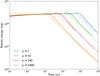 |
Fig. A.1 Total kinetic energy for the uniform simulations. The thin straight lines correspond to the analytical trends described in Sect. 3.1. |
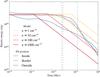 |
Fig. A.2 Kinetic energy injection: comparison between turbulent simulations and our model. The vertical lines correspond to the time at which the gas starts leaving the computational domain (from left to right: border, outside, inside). |
It is also worth studying the amount of kinetic energy that is injected into the ISM during the supernova explosions. Figure A.1 shows the total kinetic energy as a function of time. As with the momentum plots described before, we see the adiabatic phase where energy is conserved (the kinetic energy being a constant fraction of the total energy in this phase), the shell formation, and the snowplow phase where the energy of the hot dense shell is radiated away, approximately following the momentum-conserving snowplow model EK ∝ t− 3/4. The ratio between total and kinetic energy is about 0.2 − 0.3 in the adiabatic phase in good agreement with Sedov’s model.
For the momentum-conserving snowplow model, the shell radius evolves with time as Rs ∝ t1/4. This stems from the fact that p ∝ R3v, while v = dR/ dt and p is nearly constant. Therefore, the kinetic energy can be approximated by  (A.1)where EK,51 is the integrated kinetic energy in 1051 erg, E51 is the initial supernova energy in 1051 erg, t4 is the age of the remnant in 104 yr, and ttr,4 is the transition time in 104 yr.
Figure A.2 shows the evolution of kinetic energy in the turbulent case, compared to our simple model. The injected kinetic energy roughly corresponds to the uniform case in the Sedov-Taylor phase, and stays in the same order of magnitude in the radiative phase.
Appendix B: Density distributions
 |
Fig. B.1 Density probability distribution just before the explosion and at two later times. Top panel: case without supernova and bottom panel: inside run. While significant differences are seen in the diffuse gas distribution, the high-density tail is largely unchanged by the supernova explosions. |
Figure B.1 shows the density probability distribution functions in the runs without supernova (top panel) and with a supernova inside (bottom panel). As can be seen, a high-density power law with a slope between −1 and −3/2 develops. Such a power law has been found in simulations including gravity and turbulence (e.g., Kritsuk et al. 2011) and is due to the collapse itself. The supernova does not change the high-density part of the distribution, but produces very diffuse gas and hot material. This is even more clearly seen in Fig. 6, which shows the mass above various thresholds as a function of time in the four runs (without supernova, outside, border, and inside).
Appendix C: Influence of the magnetic field
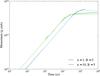 |
Fig. C.1 Integrated radial momentum for the uniform MHD simulations. The thin straight lines correspond to the analytical trends described in Sect. 3.1. |
We now study the impact that a magnetic field can have on the supernova remnant influence on the ISM. We proceed as for the hydrodynamical case starting with the uniform configuration, and then investigate the turbulent case.
Appendix C.1: Uniform case
Figure C.1 shows the differences between momentum injection with an ambient uniform magnetic field (taken to be 5 μG) and the model for n = 1 and n = 10 cm-3. The values in the final stage are almost unchanged by the presence of magnetic field. This is relatively unsurprising since as seen from the turbulent simulations, the final momentum is relatively insensitive to density variations and complex geometry. In particular, the magnetic field does not alter very significantly the shock structure as long as it remains adiabatic, nor does it modify the cooling rate.
Appendix C.2: Turbulent case
To include a magnetic field in the turbulent cloud runs, we introduce a uniform field initially. Its intensity is about 5 μG, which corresponds for the 104M⊙ cloud to an initial mass-to-flux ratio of about 10. The initial magnetic field is, however, significantly amplified before the supernova is introduced.
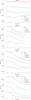 |
Fig. C.2 MHD case. Mass above densities thresholds 10,100,1000 cm-3 in the case without supernova (top panel) and outside (second panel), border (third panel) and inside (bottom panel) runs. |
 |
Fig. C.3 Integrated radial injected momentum: comparison between turbulent MHD and our model. The vertical lines correspond to the first matter outflow for each case (from left to right: border, outside, inside). |
Appendix C.2.1: Impact of the supernova remnant on the cloud
The evolution (not shown for conciseness) of the magnetized cloud is very similar to the hydrodynamical case. The supernova hot gas quickly escapes through the low-density material, whereas the high-density clumps are pushed away more slowly. A difference is that the propagation of the supernova in the diffuse medium is no longer spherical because it propagates more easily along the magnetic field lines as noted in earlier works (e.g., Tomisaka 1998).
Figure C.2 shows the mass above 3 density thresholds as a function of time for the four MHD runs. The run without supernova (top panel) is very similar to the corresponding hydrodynamical run (top panel of Fig. 6). In particular, the mass above 103 cm-3 is almost identical in the two runs.
In the two MHD runs outside and border (second and third panels), the mass of gas above 103 cm-3 is smaller than in the hydrodynamical case by a factor of about 10 − 20%. The same is true for the inside run where it is seen that the mass above 103 cm-3 rapidly drops below 5000 M⊙.
This shows that the presence of a magnetic field tends to enhance the influence supernovae have on molecular clouds, probably because the magnetic field exerts a coupling between the different fluid particles within molecular clouds. Therefore, as some gas is pushed away by the high pressure supernova remnant, more gas is entrained.
Appendix C.2.2: Momentum injection
Figure C.3 shows the evolution of the radial momentum (with respect to the supernova center) with time in the turbulent case with magnetic field. The evolution is very similar to the hydrodynamical case displayed in Fig. 5 (top panel) and reasonably well described by the simple model presented in Sect. 3.1. This confirms the result of the uniform density runs about the weak influence magnetic field has on the total momentum delivered to the ISM.
In addition to the value of the total momentum, it is important (as discussed above) to quantify the momentum distribution as a function of density. Figure C.4 shows the momentum injected for the three density thresholds as a function of time for the MHD runs. These results should be compared with Fig. 7. There are more differences than for the total momentum, particularly in the inside run for which it is seen that the momentum delivered at high density just after the supernova explosion is about 20 to 30% higher than in the hydrodynamical case. This is in good agreement with the results obtained for the mass evolution (Fig. C.2).
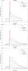 |
Fig. C.4 MHD case. Evolution of momentum for densities above thresholds 10,100, and 1000 cm-3 in the outside, border, and inside cases. |
Altogether, the various MHD runs presented in this section reveal that the magnetic field does not modify the total amount of momentum injected by supernovae into the ISM. It has a modest
impact on the momentum that is injected into the dense gas, and therefore on the impact that supernovae may have in limiting star formation, if the supernova lies inside the dense gas when it explodes. The magnetic field has almost no impact if the supernova explodes outside the denser regions.
Acknowledgments
It is a pleasure to thank Eve Ostriker for stimulating discussions and insightful suggestions, Anne Decourchelle and Jean Ballet for enlightening elements regarding the observations of supernovae remnants and Matthieu Gounelle for triggering our interest in supernova explosions. We thank the anonymous referee for a careful reading of the manuscript which has significantly improved the paper. This work was granted access to HPC resources of CINES under the allocation x2014047023 made by GENCI (Grand Equipement National de Calcul Intensif). P.H. acknowledges the financial support of the Agence Nationale pour la Recherche through the COSMIS project. This research has received funding from the European Research Council under the European Community’s Seventh Framework Programme (FP7/2007-2013 Grant Agreement No. 306483 and No. 291294).
References
- Audit, E., & Hennebelle, P. 2005, A&A, 433, 1 [NASA ADS] [CrossRef] [EDP Sciences] [Google Scholar]
- Avillez, M. A., & Breitschwerdt, D. 2005, A&A, 436, 585 [NASA ADS] [CrossRef] [EDP Sciences] [Google Scholar]
- Ballesteros-Paredes, J., Klessen, R. S., Mac Low, M.-M., & Vazquez-Semadeni, E. 2007, in Protostars and Planets V, eds. B. Reipurth, D. Jewitt, & K. Keil (Tucson: University of Arizona Press), 63 [Google Scholar]
- Blondin, J. M., Wright, E. B., Borkowski, K. J., & Reynolds, S. P. 1998, ApJ, 500, 342 [NASA ADS] [CrossRef] [Google Scholar]
- Bournaud, F., Elmegreen, B. G., Teyssier, R., Block, D. L., & Puerari, I. 2010, MNRAS, 409, 1088 [NASA ADS] [CrossRef] [Google Scholar]
- Brogan, C. L., Gelfand, J. D., Gaensler, B. M., Kassim, N. E., & Lazio, T. J. W. 2006, ApJ, 639, L25 [NASA ADS] [CrossRef] [Google Scholar]
- Chen, Y., Jiang, B., Zhou, P., et al. 2013, Invited talk, Supernova environmental impacts, Raichak-on-Ganges, India, Jan. 7–11, IAU Symp., 296 [arXiv:1304.5367] [Google Scholar]
- Chevalier, R. A. 1974, ApJ, 188, 501 [NASA ADS] [CrossRef] [Google Scholar]
- Chevalier, R. A. 1999, ApJ, 511, 798 [NASA ADS] [CrossRef] [Google Scholar]
- Chu, Y.-H., & Mac Low, M.-M. 1990, ApJ, 365, 510 [NASA ADS] [CrossRef] [Google Scholar]
- Cioffi, D. F., McKee, C. F., & Bertschinger, E. 1988, ApJ, 334, 252 [NASA ADS] [CrossRef] [Google Scholar]
- Dale, J. E., Ercolano, B., & Bonnell, I. A. 2012, MNRAS, 424, 377 [NASA ADS] [CrossRef] [Google Scholar]
- Dale, J. E., Ercolano, B., & Bonnell, I. A. 2013, MNRAS, 430, 234 [NASA ADS] [CrossRef] [MathSciNet] [Google Scholar]
- Dale, J. E., Ngoumou, J., Ercolano, B., & Bonnell, I. A. 2014, MNRAS, 442, 694 [NASA ADS] [CrossRef] [MathSciNet] [Google Scholar]
- Dobbs, C. L., Burkert, A., & Pringle, J. E. 2011, MNRAS, 417, 1318 [NASA ADS] [CrossRef] [Google Scholar]
- Dubois, Y., & Teyssier, R. 2008, A&A, 477, 79 [NASA ADS] [CrossRef] [EDP Sciences] [Google Scholar]
- Elmegreen, B. G., & Elmegreen, D. M. 1987, ApJ, 320, 182 [NASA ADS] [CrossRef] [Google Scholar]
- Fromang, S., Hennebelle, P., & Teyssier, R. 2006, A&A, 457, 371 [NASA ADS] [CrossRef] [EDP Sciences] [Google Scholar]
- Fukui, Y., Moriguchi, Y., Tamura, K., et al. 2003, PASJ, 55, L61 [NASA ADS] [Google Scholar]
- Geen, S., Rosdahl, J., Blaizot, J., Devriendt, J., & Slyz, A. 2014, MNRAS, submitted [arXiv:1412.0484] [Google Scholar]
- Gent, F. A., Shukurov, A., Fletcher, A., Sarson, G. R., & Mantere, M. J. 2013, MNRAS, 432, 1396 [NASA ADS] [CrossRef] [Google Scholar]
- Hennebelle, P., & Falgarone, E. 2012, A&ARv, 20, 55 [NASA ADS] [CrossRef] [Google Scholar]
- Hennebelle, P., & Iffrig, O. 2014, A&A, 570, A81 [NASA ADS] [CrossRef] [EDP Sciences] [Google Scholar]
- Hewitt, J. W., Yusef-Zadeh, F., & Wardle, M. 2009, ApJ, 706, L270 [NASA ADS] [CrossRef] [Google Scholar]
- Hill, A. S., Joung, M. R., Mac Low, M.-M., et al. 2012, ApJ, 750, 104 [NASA ADS] [CrossRef] [Google Scholar]
- Hopkins, P. F., Quataert, E., & Murray, N. 2011, MNRAS, 417, 950 [NASA ADS] [CrossRef] [Google Scholar]
- Joung, M. K. R., & Mac Low, M.-M. 2006, ApJ, 653, 1266 [NASA ADS] [CrossRef] [Google Scholar]
- Kim, C.-G., & Ostriker, E. C. 2014, ApJ, submitted [arXiv:1410.1537] [Google Scholar]
- Kim, C.-G., Kim, W.-T., & Ostriker, E. C. 2011, ApJ, 743, 25 [NASA ADS] [CrossRef] [Google Scholar]
- Kim, C.-G., Ostriker, E. C., & Kim, W.-T. 2013, ApJ, 776, 1 [NASA ADS] [CrossRef] [Google Scholar]
- Kritsuk, A. G., Norman, M. L., & Wagner, R. 2011, ApJ, 727, L20 [NASA ADS] [CrossRef] [Google Scholar]
- Li, Z.-Y., & Nakamura, F. 2006, ApJ, 640, L187 [NASA ADS] [CrossRef] [Google Scholar]
- Mac Low, M.-M., & Klessen, R. S. 2004, Rev. Mod. Phys., 76, 125 [NASA ADS] [CrossRef] [Google Scholar]
- Martizzi, D., Faucher-Giguère, C.-A., & Quataert, E. 2014, MNRAS, submitted [arXiv:1409.4425] [Google Scholar]
- Matzner, C. D. 2002, ApJ, 566, 302 [NASA ADS] [CrossRef] [Google Scholar]
- McKee, C. F., & Ostriker, J. P. 1977, ApJ, 218, 148 [NASA ADS] [CrossRef] [Google Scholar]
- Oort, J. H. 1951, in Problems of Cosmical Aerodynamics, 118 [Google Scholar]
- Ostriker, J. P., & McKee, C. F. 1988, Rev. Mod. Phys., 60, 1 [NASA ADS] [CrossRef] [Google Scholar]
- Renaud, F., Bournaud, F., Emsellem, E., et al. 2013, MNRAS, 436, 1836 [NASA ADS] [CrossRef] [Google Scholar]
- Rogers, H., & Pittard, J. M. 2013, MNRAS, 431, 1337 [NASA ADS] [CrossRef] [Google Scholar]
- Sedov, L. I. 1959, Similarity and Dimensional Methods in Mechanics (New York: Academic Press) [Google Scholar]
- Shull, Jr., P. 1983, ApJ, 275, 611 [NASA ADS] [CrossRef] [Google Scholar]
- Shull, Jr., P.,Dyson, J. E., Kahn, F. D., & West, K. A. 1985, MNRAS, 212, 799 [NASA ADS] [CrossRef] [Google Scholar]
- Slane, P., Bykov, A., Ellison, D. C., Dubner, G., & Castro, D. 2014, Space Sci. Rev., DOI: 10.1007/s11214-014-0062-6 [Google Scholar]
- Slyz, A. D., Devriendt, J. E. G., Bryan, G., & Silk, J. 2005, MNRAS, 356, 737 [NASA ADS] [CrossRef] [Google Scholar]
- Sutherland, R. S., & Dopita, M. A. 1993, ApJS, 88, 253 [NASA ADS] [CrossRef] [Google Scholar]
- Tasker, E. J. 2011, ApJ, 730, 11 [NASA ADS] [CrossRef] [Google Scholar]
- Tasker, E. J., & Bryan, G. L. 2006, ApJ, 641, 878 [NASA ADS] [CrossRef] [Google Scholar]
- Teyssier, R. 2002, A&A, 385, 337 [NASA ADS] [CrossRef] [EDP Sciences] [Google Scholar]
- Tomisaka, K. 1998, MNRAS, 298, 797 [NASA ADS] [CrossRef] [Google Scholar]
All Tables
Transition time ttr and final momentum pf as a function of the ambient density n0.
All Figures
|
Fig. 1 Positions of the supernovae injected in the cloud simulations. |
| In the text | |
|
Fig. 2 Integrated radial momentum for the uniform simulations. The thin straight lines correspond to the analytical trends described in Sect. 3.1. Two main phases can be distinguished. First, during the Sedov-Taylor phase the momentum increases with time. Then, during the radiative snowplow phase the momentum is nearly constant. The dependence of the momentum on the ISM density is rather shallow. |
| In the text | |
|
Fig. 3 Column density maps for the turbulent hydrodynamical simulations. Top panel: no supernova, 0.27,0.85,1.4 Myr after injection time; middle panel: supernova inside; bottom panel: supernova outside, both after 100, 200 and 750 kyr. |
| In the text | |
|
Fig. 4 Temperature maps for the turbulent hydrodynamical simulations 1, 20 and 100 kyr after supernova injection time. Top panel: supernova inside; bottom panel: supernova outside (in this view the explosion takes place behind the cloud). |
| In the text | |
|
Fig. 5 Top panel: total radial momentum, comparison between turbulent simulations and the analytical model for various densities. The vertical lines correspond to the time at which the gas starts leaving the computational domain (from left to right: border, outside, inside). Bottom panel: inside run for two different box sizes and two numerical resolutions. |
| In the text | |
|
Fig. 6 Mass above density thresholds 10,100,1000 cm-3 in the case without supernova (top panel) and outside (second panel), border (third panel) and inside (bottom panel) runs. |
| In the text | |
|
Fig. 7 Evolution of momentum for densities above thresholds 10,100, and 1000 cm-3 in the outside, border, and inside cases. |
| In the text | |
|
Fig. A.1 Total kinetic energy for the uniform simulations. The thin straight lines correspond to the analytical trends described in Sect. 3.1. |
| In the text | |
|
Fig. A.2 Kinetic energy injection: comparison between turbulent simulations and our model. The vertical lines correspond to the time at which the gas starts leaving the computational domain (from left to right: border, outside, inside). |
| In the text | |
|
Fig. B.1 Density probability distribution just before the explosion and at two later times. Top panel: case without supernova and bottom panel: inside run. While significant differences are seen in the diffuse gas distribution, the high-density tail is largely unchanged by the supernova explosions. |
| In the text | |
|
Fig. C.1 Integrated radial momentum for the uniform MHD simulations. The thin straight lines correspond to the analytical trends described in Sect. 3.1. |
| In the text | |
|
Fig. C.2 MHD case. Mass above densities thresholds 10,100,1000 cm-3 in the case without supernova (top panel) and outside (second panel), border (third panel) and inside (bottom panel) runs. |
| In the text | |
|
Fig. C.3 Integrated radial injected momentum: comparison between turbulent MHD and our model. The vertical lines correspond to the first matter outflow for each case (from left to right: border, outside, inside). |
| In the text | |
|
Fig. C.4 MHD case. Evolution of momentum for densities above thresholds 10,100, and 1000 cm-3 in the outside, border, and inside cases. |
| In the text | |
Current usage metrics show cumulative count of Article Views (full-text article views including HTML views, PDF and ePub downloads, according to the available data) and Abstracts Views on Vision4Press platform.
Data correspond to usage on the plateform after 2015. The current usage metrics is available 48-96 hours after online publication and is updated daily on week days.
Initial download of the metrics may take a while.