| Issue |
A&A
Volume 576, April 2015
|
|
|---|---|---|
| Article Number | A96 | |
| Number of page(s) | 8 | |
| Section | Numerical methods and codes | |
| DOI | https://doi.org/10.1051/0004-6361/201424194 | |
| Published online | 10 April 2015 | |
Restricted Boltzmann machine: a non-linear substitute for PCA in spectral processing⋆
1
Key Laboratory of Optical Astronomy, National Astronomical Observatories,
Chinese Academy of Sciences,
100012
Beijing,
PR China
e-mail:
This email address is being protected from spambots. You need JavaScript enabled to view it.
2
School of Mathematics and Statistics, Shandong University,
Weihai,
264209, Shandong, PR China
3
School of Mechanical, Electrical & Information
Engineering, Shandong University, Weihai, 264209, Shandong,
PR China
Received: 13 May 2014
Accepted: 17 February 2015
Abstract
Context. Principal component analysis (PCA) is widely used to repair incomplete spectra, to perform spectral denoising, and to reduce dimensionality. Presently, no method has been found to be comparable to PCA on these three problems. New methods have been proposed, but are often specific to one problem. For example, locally linear embedding outperforms PCA in dimensionality reduction. However, it cannot be used in spectral denoising and spectral reparing. Wavelet transform can be used to denoise spectra; however, it cannot be used in dimensionality reduction.
Aims. We provide a new method that can substitute PCA in incomplete spectra repairing, spectral denoising and spectral dimensionality reduction.
Methods. A new method, restricted Boltzmann machine (RBM), is introduced in spectral processing. RBM is a particular type of Markov random field with two-layer architecture, and use Gibbs sampling method to train the algorithm. It can be used in spectral denoising, dimensionality reduction and spectral repairing.
Results. The performance of RBM is comparable to PCA in spectral processing. It can repair the incomplete spectra better: the difference between the RBM repaired spectra and the original spectra is smaller than that between the PCA repaired spectra and the original spectra. The denoised spectra given by RBM is similar to those given by PCA. In dimensionality reduction, RBM performs better than PCA: the classification results of RBM+ELM (i.e. the extreme learning machine) is higher than those of PCA+ELM. This shows that RBM can extract the spectral features more efficiently than PCA. Thus, RBM is a good alternative method for PCA in spectral processing.
Key words: methods: statistical / methods: data analysis / methods: numerical
The source code of RBM algorithm is only available at the CDS via anonymous ftp to cdsarc.u-strasbg.fr (130.79.128.5) or via http://cdsarc.u-strasbg.fr/viz-bin/qcat?J/A+A/576/A96
© ESO, 2015
1. Introduction
With the development of modern astronomical instruments, we can obtain huge amounts of data. For example, Sloan Digital Sky Survey (SDSS; York et al. 2000) has provided us with millions of high dimensional spectra, including a large amount of incomplete data and noisy data. How to deal with these high dimensional, noisy, and incomplete data efficiently and automatically is a main difficulty that needs to be overcome. Principal component analysis (PCA) is among the most widely used linear techniques in (1) reducing the dimension of spectra; (2) denoising the spectra; (3) repairing the incomplete spectra.
Principal component analysis is widely used to reduce the spectral dimension. It is often used as a prepared procedure in spectral classification. That is, PCA is often the first step in the spectral classification. For example, it has been used in stellar spectral classification (Deeming 1964; Whitney 1983), galaxy spectral classification (Connolly et al. 1995; Lahav et al. 1996; Connolly & Szalay 1999; Yip et al. 2004b; Ferreras et al. 2006; Chen et al. 2012), and quasar spectral classification (Yip et al. 2004a; Francis et al. 1992). However, since PCA is a linear method, it may not be efficient enough to describe the non-linear properties within the spectra. For example, PCA is not able to describe the high-frequency structure of the spectrum, such as lines ratios and line widths. Thus, some non-linear methods, such as the manifold learning method, have been introduced in the spectral dimensionality reduction. Vanderplas & Connolly (2009) employed locally linear embedding (LLE) method to classify the galaxy and QSO spectra. They found that LLE can project the QSOs and galaxies into different regions. Furthermore, it successfully separates the broad line galaxies from the narrow line ones in two-dimensional space, which is impossible for PCA. Daniel et al. (2011) employed LLE to classify the stellar spectra. They found that the majority of stellar spectra can be represented as one LLE dimensional sequence, and this sequence correlates well with the spectral temperature. However, it is worth noting that, unlike PCA, the above manifold learning algorithm cannot provide the eigenspectra like PCA. Thus, it is difficult for us to determine the connection between the components given by the manifold learning algorithm and the physical properties of the spectra. Furthermore, we cannot apply the manifold learning algorithm to denoise the spectra and repair the incomplete spectra.
The PCA technique has also been used to process the noisy and incomplete data. Yip et al. (2004b) applied PCA to deal with galaxy spectra with gaps. They first fixed the gaps of the spectra by other methods, e.g. linear interpolation. Then they constructed a set of eigenspectra from the gap-repaired spectra. Then the gaps of the original spectra are corrected with the linear combination of the eigenspectra. The whole process is iterated until the eigenspectra converge. Yip et al. (2004a) used a similar method to deal with the incomplete quasar spectra. Connolly & Szalay (1999) used PCA to deal with the incomplete and noisy galaxy spectra. They repaired the incomplete spectra by minimizing the weighted difference between the original spectra and the reconstructed spectra, and found that this method provides the best interpolation of galaxy spectra over the missing data and an optimal filtering of a noisy spectrum. To estimate the stellar atmospheric parameters accurately, Re Fiorentin et al. (2007) applied PCA to filter the noise and recover missing features of the spectra. The results show that using 25 eigenspectra PCA can filter the noise of spectra and reconstruct the spectra accurately. Thus, PCA is an efficient method for processing noisy and incomplete spectral data.
In this paper, we introduce a new method, the restricted Boltzmann machine (RBM), to the spectral processing. This method was invented by Smolensky (1986), and is now a widely used pattern recognition method after Hinton and collaborators invented fast learning algorithms for RBM in 2006 (Hinton et al. 2006). It has been applied in dimensionality reduction (Hinton & Salakhutdinov 2006), classification (Larochelle & Bengio 2008), collaborative filtering (Salakhutdinov et al. 2007), and feature learning (Coates et al. 2011). In Chen et al. (2014), RBM has been used to classify the cataclysmic variables from other types of spectra. The result shows state-of-the-art accuracy of 100%, which indicates the efficiency of RBM in spectral classification. In this paper, we investigate the performance of RBM in spectral processing. Experiments show that the performance of RBM in repairing incomplete spectra, spectral denoising, and spectral dimensionality reduction is comparable with that of PCA, and thus RBM is a good alternative to PCA.
The paper is organized as follows. In Sect. 2, we provide a brief introduction to RBM, PCA, and the extreme learning machine (ELM) method. In Sect. 3, we describe the spectral data we used in the experiment. In Sect. 4, we compare performance of RBM with that of PCA in incomplete spectra repair, spectral denoising, and dimensionality reduction. In Sect. 5, we compare RBM with other widely used methods such as the manifold learning method, and discuss the possible applications of RBM. Section 6 concludes the paper.
2. Methods
In this section, we give a brief introduction to RBM (see Bengio 2009 for more details), PCA (see Jolliffe 2005), and ELM (see Huang et al. 2006).
2.1. Restricted Boltzmann machine
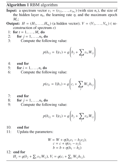
In this section, we present the definition and the fast learning algorithm of RBM. A practical algorithm of RBM is given in Appendix A. To facilitate the implementation of RBM, a source code of RBM algorithm written in Matlab is provided as the supplementary material of this paper and is available at the CDS.
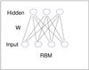 |
Fig. 1 Restricted Boltzmann machine. |
2.1.1. What is RBM
A restricted Boltzmann machine is a particular type of Markov random field with two-layer architecture, in which the visible, binary stochastic vector v ∈ Rnv is connected to the hidden binary vector h ∈ Rnh, where nv is the size of v and nh is the size of h (Fig. 1). In the paper, the visible vector corresponds to the spectrum, and the hidden vector corresponds to the output of RBM. We will define the units in the hidden vector as the RBM components. Suppose that θ = { W,b,a } are the model parameters: Wij represents the symmetric interaction term between visible unit vi and hidden units hj; and bi and aj are the biases of visible and hidden units, respectively. The joint distribution over the visible and hidden units is defined by 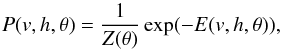 (1)where Z(θ) = ∑ v ∑ hexp(−E(v,h,θ)) is known as the partition function or normalizing constant. Then, the distribution of hidden units h given the visible units v is
 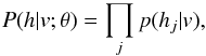 where
where 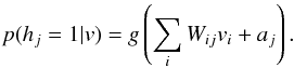 (2)Here g(x) = 1 / (1 + exp(−x)) is the logistic function. The distribution of the visible units v given the hidden units h is
  where
where  (3)Through Eq. (2), once we know the weight matrix W = (Wij) (i = 1,...,nv,j = 1,...,nh) and the hidden bias aj (j = 1,...,nh), we can get the values of hidden units from the visible units. Through Eq. (3), if we also know visible bias bi(i = 1,...,nv), we can get the value of visible units from the value of hidden units. Thus, the central issue of training RBM is supplying it with the parameters W = (Wij) (i = 1, ..., nv,j = 1,..., nh), aj(j = 1, ..., nh), and bi (i = 1, ..., nv), i.e. parameter θ. We will show how to train RBM in the following section.
2.1.2. How to train RBM
From above discussion, we know that the main issue of teaching a RBM is to learn the parameter θ. We define  where P(v,θ) represents the probability of visible units (data). Since P(v,θ) describes the distribution of the data, we learn θ to maximize the P(v,θ), or log P(v,θ) equivalently. We use the gradient descent method to learn parameters to maximize P(v,θ). We only show how to learn W; the way to learn the other parameters is similar. The gradient of object function log P(v,θ) with respect to W is
 ![Mathematical equation: \begin{equation} \label{e4} \frac{\partial\log P(v,\theta)}{\partial W}=E_{\rm data}[vh^T]-E_{\rm model}[vh^T], \end{equation}](/articles/aa/full_html/2015/04/aa24194-14/aa24194-14-eq31.png) (4)where Edata denotes the expectation with respect to the data distribution
(4)where Edata denotes the expectation with respect to the data distribution  with Pdata the empirical distribution. The transpose of matrix is represented by T and Emodel is the expectation with respect to the distribution defined by the model as in Eq. (1). The proof of Eq. (4) can be found in Bengio (2009). However, it is not easy to compute the Emodel [ vhT ]. Then, as proposed in Hinton et al. (2006), we use
 ![Mathematical equation: \begin{eqnarray*} \Delta W=\eta\left(E_{\rm data}\left[vh^T\right]-E_G\left[vh^T\right]\right) \end{eqnarray*}](/articles/aa/full_html/2015/04/aa24194-14/aa24194-14-eq38.png) to approximate Eq. (4), where EG represents the expectation with respect to a distribution PG defined by running a G-step Gibbs chain sample that starts at the data.
to approximate Eq. (4), where EG represents the expectation with respect to a distribution PG defined by running a G-step Gibbs chain sample that starts at the data.
We first show how to compute Edata [ vhT ]. We denote the input spectra vector as v0, and set the initial weights W and bias term a and b randomly. By using these random weights and the bias term we can get the hidden vector h0 from the input data v0 by using Eq. (2). Then, ![Mathematical equation: \hbox{$E_{\rm data}[vh^T]=v_0h^T_{0}$}](/articles/aa/full_html/2015/04/aa24194-14/aa24194-14-eq47.png) .
.
We now show how to compute EG [ vhT ], that is, how we use Gibbs sample technique to compute EG [ vhT ]. We set the first step visible states v0 = data and use Eq. (2) to obtain the first round hidden states h0. From h0 and Eq. (3) we can obtain the second round visible state v1 and from v1 we can get h1, and so on. This procedure is shown in Fig. 2. If we run a G-step Gibbs sample, we will get the G round visible and hidden value vG and hG, and further we can obtain ![Mathematical equation: \hbox{$E_G[vh^T]=v_Gh_G^T$}](/articles/aa/full_html/2015/04/aa24194-14/aa24194-14-eq54.png) . In practice, we set G = 1. That is, using
. In practice, we set G = 1. That is, using  as an estimate of Emodel [ vhT ] performs well in practice.
When training RBM, no label information is involved. Thus, RBM is an unsupervised algorithm, which is same as PCA. Similar to PCA, RBM can be used to project the high dimensional spectra into low dimensional space. The hidden layer vectors given by RBM are similar to the PC vectors given by PCA. If we set the size of the hidden layer of RBM to be 1000, then we will project the spectra into a 1000 dimensional space given by RBM and the corresponding hidden layer vectors are the 1000 dimensional representation of the spectra. We then define the RBM dimension to be the size of the hidden layer, and the RBM components correspond to the components in the hidden layer vector. We use R1 to represent the first RBM component, R2 to represent the second RBM component, and so on.
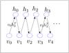 |
Fig. 2 Practical procedure for learning RBM. |
2.2. Principal component analysis
In this section, we give a brief introduction to PCA. We first show how to obtain the principal components. We suppose that X = (X1,...,Xn)T is the data set, where  is a spectrum with m flux bins. We can compute the matrix
  where
where  is the so-called centring matrix, E is the identity matrix, and AO is a matrix with all of its elements equal to 1; A is a diagonal matrix
  i.e. its diagonal element is
  where
where  and
and  . Then we can renew X with Xs. After renewing X, we need to compute the eigenvalues of covariance matrix XTX, where XT is the transpose of the matrix X. We let Em × m be the eigenvector matrix of the covariance matrix XTX. Then the principal component matrix P can be obtained by
  (5)We now show how to obtain the reconstruction of the data by using the first k principal components. From Eq. (5) we have X = PE-1. If we set the last m − k rows of E-1 to be zero, we can obtain a matrix E∗. We let X∗ = PE∗. Then X∗ is the reconstructed matrix of X using the first k principal components. If we define pij to be the element in the ith row and jth column of P,
  to be the ith row of X∗ and
  the jth row of E∗, and then we have
2.3. Extreme learning machine
We will use ELM as the classifier in the experiment to classify the spectra into different types. We now give a short introduction to ELM.
Suppose that { xi,yi } (i = 1...,N) is the data set, where xi = (xi1,...,xin)T ∈ Rn is a spectrum with n dimension and yi is the target value corresponding to xi. The standard single-hidden layer feedforward neural network (SLFNs) with S hidden nodes and activation function g(x) can be formulated as 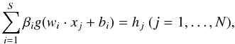 (6)where hj (j = 1,...,N) is the output of SLFNs. We define
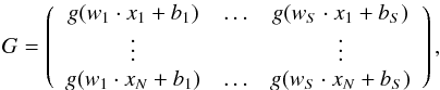
 and
and 
where βi (i = 1,2,...,S) and hi (i = 1,2,...,n) are columns with m elements. Then Eq. (6) can be written as Gβ = H.
We seek the optimal parameters which can minimize the difference between the output of SLFNs and the target vectors. That is, we have to search  , and
, and  such that
  where
where ![Mathematical equation: \hbox{$Y=[y_1,\ldots,y_N]^T_{N\times 1}$}](/articles/aa/full_html/2015/04/aa24194-14/aa24194-14-eq109.png) . The traditional method, e.g. gradient-based learning algorithms, is to search optimal wi,bi, and β. This is used in BP algorithm, and has proved to be time-comsuming. However, in ELM algorithm, instead of searching for all the optimal parameters, only the optimal β will be given. Parameters wi and bi can be set randomly and will not be optimized. This saves a significant amount of training time and improves the efficiency of training.
. The traditional method, e.g. gradient-based learning algorithms, is to search optimal wi,bi, and β. This is used in BP algorithm, and has proved to be time-comsuming. However, in ELM algorithm, instead of searching for all the optimal parameters, only the optimal β will be given. Parameters wi and bi can be set randomly and will not be optimized. This saves a significant amount of training time and improves the efficiency of training.
We have compared ELM with BP and cluster algorithm. The result is shown in Fig. 3. The data we used in the experiment have been preprocessed with RBM. We find that ELM is more efficient and accurate than other two methods. The experiment on data preprocessed with PCA gives a similar conclusion. Thus, ELM will be used as the classifier in our experiments, and the classification results will then be used to assess the performance of PCA and RBM in dimensionality reduction.
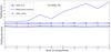 |
Fig. 3 Upper panel: time that three algorithms take for classification versus the number of RBM components. The vertical axis represents the time that the computer takes for testing, while the horizontal axis represents the number of RBM components used in the experiment. The RBM components are obtained by applying RBM to the spectral data, and it is similar to the PCA components. Lower panel: testing accuracies of the three algorithms versus the number of RBM components. The vertical axis represents the testing accuracies, while the horizontal axis represents the number of RBM components used in experiments. We only present the results of using spectra data with 10 <S/N ≤ 20. We note that the results of using other data sets and using the PCA components are similar to the results present here. |
3. Data
The SDSS is an imaging and spectroscopic survey of the high Galactic latitude sky visible from the northern hemisphere. It uses a dedicated wide-field 2.5 m telescope at Apache Point Observatory in south-east New Mexico. To date, SDSS has provided us millions of spectra. The spectra we used in experiments are from the ninth data release of SDSS (SDSS DR9; Ahn et al. 2012). These spectra cover the full SDSS provided wavelength range 3800–9200 Å, in 3759 individual data bins. The resolution of the spectra is 1500 at 3800 Å and 2500 at 9000 Å. We have not taken any further steps such as continuum subtraction to preprocess the spectra except normalizing the spectra to a constant total flux.
The data we used consists of two parts, one part is used for repairing, and the other is used for denoising. The data used for repairing contains three data sets: D1, consists of the spectra with signal-to-noise ratios (S/N) larger than 20; D2, consists of the spectra with 10 <S/N ≤ 20; D3, consists of the spectra with S/N ≤ 10. Because of the limitation of computational power, each data set contains 9000 spectra: 3000 stellar spectra, 3000 galaxy spectra, and 3000 QSOs spectra. These 3000 stellar spectra contain 2000 early-type spectra (F or A type) and 1000 late-type spectra (M type). The galaxy spectra contain 1000 starforming-type spectra, 1000 starburst-type spectra, and 1000 AGN-type spectra. The detailed information of these data sets are given in Table 1. The data used for denoising has a same structure as the data used for repairing. We denote them as D4 (S/N> 20), D5 (10 <S/N ≤ 20), and D6 (0 <S/N ≤ 10).
Distribution of data set D1.
4. Results: RBM and PCA in comparison
4.1. Repairing incomplete data
The observed galaxy spectra and QSO spectra often cover a broad range of rest wavelengths, have variable signal-to-noise ratios, and contain spectral regions affected by sky lines or artifacts in the spectrographs. This will result in spectra with gaps or missing spectral regions. Thus, we have to repair the incomplete spectra before further processing these data such as spectral classification and redshift measurement. In this section, we will show the performance of RBM in repairing the spectra and then make a comparison with PCA.
To quantify the performance of RBM and PCA, we perform the following steps to process the data and measure the performance of RBM and PCA:
-
1.
We randomly select n spectra Ti (i = 1,...,n), and for each spectrum we randomly set the flux at m contiguous wavelength bins to be zeros; that is, the missing region of each spectrum covers m contiguous wavelength bins. We then obtain n pseudo-incomplete spectra, which is denoted as Ii (i = 1,2,...,n).
-
2.
Using RBM and PCA to the spectra to repair the pseudo-incomplete spectra. We denote the repaired spectra as Ri (i = 1,2,...,n).
-
3.
We measure the mean difference between the flux values of the repaired spectra and that of the true spectra in the missing region using the formula
 where
Tij is the flux
values of the ith true spectra at the jth wavelength bin in
the missing region, and Rij is the flux
values of the repaired spectra corresponding to Tij. Here
j is
the index number of missing flux.
where
Tij is the flux
values of the ith true spectra at the jth wavelength bin in
the missing region, and Rij is the flux
values of the repaired spectra corresponding to Tij. Here
j is
the index number of missing flux.
-
1.
We find that the M values of D1, D2, and D3 given by RBM are significantly smaller than the corresponding values given by PCA. The maximum error given by RBM is about half of the minimum error given by PCA. Thus, RBM can recover the incomplete part of the spectra better than PCA.
-
2.
PCA performs best on data set D3 (S/N ≤ 10), while RBM performs worst on this data set. This may be because PCA is a linear algorithm, and hence can better recover the line information within the spectra. RBM is a non-linear method, and is not efficient at extracting the line features. Thus, RBM performs worst on the spectra with low S/N whose features are dominated by lines, while PCA performs best on these spectra.
-
3.
Both of the M values given by PCA and RBM will not decrease with the increasing number of components used in repairing. Thus, the first 100 components contain adequate information to repair the spectra. Then, in incomplete spectra repairing we do not need to use too many components.
It is worth noting that we can further improve the performance of PCA and RBM by using iterated steps. Namely, we can use the repaired spectra as input of RBM and PCA to repair the spectra once again. We do not discuss it here because more detailed studies are needed to address this problem.
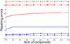 |
Fig. 4 Repairing errors of (from top to bottom) (1) PCA on spectra with 10 <S/N ≤ 20; (2) PCA on spectra with S/N> 20; (3) PCA on spectra with 0 <S/N ≤ 10; (4) RBM on spectra with 0 <S/N ≤ 10; (5) RBM on spectra with S/N> 20; and (6) RBM on spectra with 10 <S/N ≤ 20. The repairing error is the average difference between the repaired spectra and the true spectra in the missing region. From the figure we find that the repairing errors given by RBM are significantly smaller than those given by PCA. Furthermore, RBM performs worst on data set D3 (S/N ≤ 10), while PCA performs best on D3, possibly because PCA is a linear method, as opposed to RBM which is a non-linear method. Thus, PCA performs best on D3 whose principal feature is line. |
 |
Fig. 5 Incomplete spectrum, the true spectrum, and the spectra repaired by RBM and PCA. The left panel shows a stellar spectrum, the middle panel shows a galaxy spectrum, and the right panel shows a QSO spectrum. These spectra are selected from D1 (S/N> 20). The incomplete spectra are obtained by setting the fluxes of the true spectra at 300 contiguous wavelength bins to zero. |
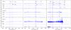 |
Fig. 6 Comparison of denoised spectra given by RBM and PCA. The denoised spectra are obtained by using 1000 RBM components or PCs. The left panels show the results on stellar spectra, the middle panels show the results on galaxy spectra, and the right panels show the results on QSOs spectra. The figures show that in the denoising procedure PCA is more efficient at recovering the narrow line features, while RBM can better recover the broadband features. This indicates that RBM can be used to process the spectra with broadband features, such as the spectra of late-type stars. We have used other numbers of components to denoise spectra and find that the difference between these results is negligible. |
4.2. Spectral denoising
To minimize the effect of noise such as the skylines, PCA is often used to denoise the spectra. In this section, we will explore the performance of RBM in filtering spectral noise. The data used for denoising are D4 (S/N> 20), D5 (10 <S/N ≤ 20), and D6 (S/N ≤ 10). We will use 1000 RBM components and PCs to denoise the spectra. We have used other numbers of components, and the results are similar.
Some examples of the denoised spectra given by RBM and PCA as well as the corresponding original spectra are shown in Fig. 6. For each spectral type (star, galaxy, or QSO) we select three spectra with different S/N to show in the figure in order to demonstrate the performance of RBM as a function of S/N. The left panels show the stellar spectra, the middle panels show the galaxy spectra, and the right panels show the QSOs spectra. The important spectral lines such as Na, Li, and Mg are marked in the figure. We find that the performance of RBM is comparable to that of PCA. Both RBM and PCA have retained the important spectral lines in the denoised spectra. Furthermore, the performance of both RBM and PCA become worse with decreasing S/N. From Fig. 6, we find that RBM can better extract broad line features, while PCA can better retain narrow line information because RBM is a non-linear algorithm, as opposed to PCA, which is a linear algorithm. This indicates that we can apply RBM to denoise the spectra whose prominent features are dominated by broadband lines, like the late-type stellar spectra. PCA performs better in denoising the spectra whose features are dominated by narrow lines, like early-type stellar spectra and galaxy spectra.
It is worth noting that some weak spectral features are often filtered along with noise lines. Thus, all these denoising methods can only help to extract the most important feature, but they often miss the subtle (weak) features. The fundamental way to solve this problem is to establish the noise model.
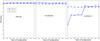 |
Fig. 7 Classification results of ELM+RBM (solid lines) and PCA+ELM (dot-dashed lines) on data sets with different S/N. The results show that RBM+ELM performs better than PCA+ELM on data sets with S/N> 20 and 10 <S/N ≤ 20. For the data set with 0 <S/N ≤ 10, RBM+ELM performs worse than PCA+ELM when using less than 600 components and performs better than PCA+ELM when using more than 600 components. |
4.3. Dimensionality reduction
In this section, we will compare the performance of RBM with that of PCA in terms of classification accuracy. That is, we will first use RBM and PCA to reduce the dimension of the spectra, and use these data to classify the spectra into different types. The classification accuracies will then be used as a measure of performance of PCA and RBM in dimensionality reduction. The dimension of data we used in classification is from 100 to 1000, with a step length of 100. The data sets used for classification are D4, D5, and D6. Each data set will be randomly divided into two equal sets, one for training and the other for testing. The classifier we use is ELM, and we classify the data into three types: galaxy, star, and QSO. The classification results are shown in Fig. 7. From the figure, we have the following two observations:
-
1.
The RBM+ELM performs better than PCA+ELM on the data sets with S/N> 10. Increasing the number of used components will not significantly improve the classification accuracy on these data sets.
-
2.
The accuracies of RBM+ELM and PCA+ELM will decrease with the decreasing of S/N. Both RBM+ELM and PCA+ELM perform worse on data sets with low S/N than on the data sets with high S/N. Figure 7 shows that RBM+ELM performs worse than PCA+ELM on data sets with S/N ≤ 10 when using less than 600 components.
5. Discussion
There are several alternative methods available with which to process the spectra. To repair incomplete spectra, we can use the Bayesian approach (Nolan et al. 2006). However, in the Bayesian method we need to determine the optimal algorithm parameters for each type of spectra. Furthermore, some prior assumptions such as the spectral factors following the Gaussian distribution are needed in the Bayesian framework to recover the missing values. It is often difficult to determine the appropriate distribution for each type of spectra. Thus, the Bayesian method is not easy to use in practice. The main advantage of RBM over the Bayesian approach is that it can treat the whole spectra data set entirely, not separately, which can save a large amount of the time spent on determining the optimal parameters.
For spectral denoising, we can use the wavelet analysis method (Qin et al. 2001; Xing & Guo 2006). However, as is well known, in wavelet analysis, each spectrum has to be denoised separately. Since we need to determine the best wavelet basis for each type of spectra, wavelet analysis is very difficult to use in practice. Compared with wavelet analysis, RBM can process the entire data set together. We do not need to determine the optimal parameter separately for each spectrum. From this point of view, RBM is simpler to use than wavelet analysis in practice.
For dimensionality reduction, we can use manifold learning methods such as LLE and the Isomap algorithm to reduce the dimension of spectra (Vanderplas & Connolly 2009; Daniel et al. 2011; Bu et al. 2013, 2014b,a). However, as shown in these studies, the manifold learning algorithm is sensitive to the noise. It often performs poorly on spectra with low S/N. However, RBM is robust against the noise. Thus, RBM performs better than manifold learning methods from this point of view.
Though RBM performs well in spectral processing, it is worth noting that there are some disadvantages of RBM compared to PCA. In PCA, we acquire the eigenbaisises, and use these eigenbaisises to obtain different PCs. However, in RBM, we cannot give the same eigenbasis. Thus, once we want to use different RBM components, we have to repeatedly run RBM. This is time consuming, and is the main disadvantages of RBM over PCA. Furthermore, eigenbasis given by PCA can be used to measure the redshift of QSOs and galaxies (Glazebrook et al. 1998). However, it is difficult for us to apply RBM to determine the redshift. This is another disadvantage of RBM over PCA.
It is worth noting that there are also some improved algorithms for PCA and RBM. For example, the kernel PCA method is proposed as an extension of PCA to process the non-linear data (Ishida & de Souza 2013). Deep belief network (DBN) is proposed as an extension of RBM to process the data with deep architectures (Hinton & Salakhutdinov 2006). The detailed comparison of RBM with these methods is beyond the scope of the paper, and we will not discuss these methods further.
We plan to further explore the application of RBM in spectral classification in the near future. We can focus on the application of RBM only to some specific spectral types, such as the supernovae and cataclysmic variables. This could extend the application of RBM. We can also use RBM to separate the spectra into subclasses. For example, we can use RBM to classify G-type stars into G2, G5, and G9; F-type stars into F2, F5, and F9; and so on.
6. Conclusion
We introduced a new method RBM for spectral processing, and compared the performance of RBM with that of PCA on incomplete spectra repairing, spectral denoising and spectral dimensionality reduction. For incomplete spectra repairing, we use the differences between the repaired values given by RBM and PCA and the true values in missing region to measure the performance of RBM and PCA. The results show that RBM can better recover the missing values. In spectral denoising, we find that the performance of RBM is comparable to PCA. Furthermore, we find that RBM is efficient at filtering the noisy lines and recovering the continuum information. In dimensionality reduction, we used RBM and PCA as the preprocessing step in spectral classification and used the classification results to measure the performance of RBM and PCA in dimensionality reduction. The results show that RBM can reliably preserve the spectral features in dimensionality reduction. Thus, RBM is a good alternative method for PCA in spectral processing. Further analysis shows that RBM can better extract the broadband spectral features, while PCA can better extract the narrow line features.
Acknowledgments
This work is supported by National Natural Science Foundation of China under grants numbers: U1431102, 11233004, 11390371 and partially supported by Independent Innovation Foundation of Shandong University (2014ZQXM015) and the Strategic Priority Research Program “The Emergence of Cosmological Structures” of the Chinese Academy of Sciences under grant No. XDB09000000. The authors are very grateful to the anonymous reviewer for a thorough reading, many valuable comments and helpful suggestions. The data used are from SDSS-III. Funding for SDSS-III has been provided by the Alfred P. Sloan Foundation, the Participating Institutions, the National Science Foundation and the US Department of Energy Office of Science. The SDSS-III web site is http://www.sdss3.org/.
References
- Ahn, C. P., Alexandroff, R., Allen de Prieto, C., et al. 2012, ApJS, 203, 21 [NASA ADS] [CrossRef] [Google Scholar]
- Bengio, Y. 2009, Foundations and Trends in Machine Learning, 2, 1 [Google Scholar]
- Bu, Y., Pan, J., Jiang, B., & Wei, P. 2013, Publ. Astron. Soc. Japan, 65, 81 [NASA ADS] [CrossRef] [Google Scholar]
- Bu, Y., Chen, F., & Pan, J. 2014a, New Astron., 28, 35 [NASA ADS] [CrossRef] [Google Scholar]
- Bu, Y.-D., Pan, J.-C., & Chen, F.-Q. 2014b, Spectroscopy and Spectral Analysis, 34, 267 [Google Scholar]
- Chen, Y.-M., Kauffmann, G., Tremonti, C. A., et al. 2012, MNRAS, 421, 314 [NASA ADS] [Google Scholar]
- Chen, F.-Q., Wu, Y., Bu, Y.-D., & Zhao, G.-D. 2014, PASA, 31, 1 [Google Scholar]
- Coates, A., Ng, A. Y., & Lee, H. 2011, in Int. Conf. Artificial Intelligence and Statistics, 215 [Google Scholar]
- Connolly, A., & Szalay, A. 1999, AJ, 117, 2052 [NASA ADS] [CrossRef] [Google Scholar]
- Connolly, A. J., Szalay, A. S., Bershady, M. A., Kinney, A. L., & Calzetti, D. 1995, AJ, 110, 1071 [NASA ADS] [CrossRef] [Google Scholar]
- Daniel, S. F., Connolly, A., Schneider, J., Vanderplas, J., & Xiong, L. 2011, AJ, 142, 203 [NASA ADS] [CrossRef] [Google Scholar]
- Deeming, T. J. 1964, MNRAS, 127, 493 [NASA ADS] [Google Scholar]
- Ferreras, I., Pasquali, A., De Carvalho, R. R., De La Rosa, I. G., & Lahav, O. 2006, MNRAS, 370, 828 [NASA ADS] [CrossRef] [Google Scholar]
- Francis, P. J., Hewett, P. C., Foltz, C. B., & Chaffee, F. H. 1992, ApJ, 398, 476 [NASA ADS] [CrossRef] [Google Scholar]
- Glazebrook, K., Offer, A. R., & Deeley, K. 1998, ApJ, 492, 98 [NASA ADS] [CrossRef] [Google Scholar]
- Hinton, G. E., & Salakhutdinov, R. R. 2006, Science, 313, 504 [NASA ADS] [CrossRef] [MathSciNet] [PubMed] [Google Scholar]
- Hinton, G. E., Osindero, S., & Teh, Y.-W. 2006, Neural Comput., 18, 1527 [Google Scholar]
- Huang, G.-B., Zhu, Q.-Y., & Siew, C.-K. 2006, Neurocomputing, 70, 489 [CrossRef] [Google Scholar]
- Ishida, E. E., & de Souza, R. S. 2013, MNRAS, 430, 509 [NASA ADS] [CrossRef] [Google Scholar]
- Jolliffe, I. 2005, Principal component analysis (Wiley Online Library) [Google Scholar]
- Lahav, O., Naim, A., Sodré, Jr., L., & Storrie-Lombardi, M. C. 1996, MNRAS, 283, 207 [NASA ADS] [CrossRef] [Google Scholar]
- Larochelle, H., & Bengio, Y. 2008, in Proc. 25th Int. Conf. on Machine Learning (NewYork: ACM), 536 [Google Scholar]
- Nolan, L. A., Harva, M. O., Kabán, A., & Raychaudhury, S. 2006, MNRAS, 366, 321 [NASA ADS] [CrossRef] [Google Scholar]
- Qin, D., Hu, Z., & Zhao, Y. 2001, in Object Detection, Classification, and Tracking Technologies, eds. J. Shen, S. Pankanti, & R. Wang, SPIE Conf. Ser., 4554, 268 [Google Scholar]
- Re Fiorentin, P., Bailer-Jones, C. A. L., Lee, Y. S., et al. 2007, A&A, 467, 1373 [NASA ADS] [CrossRef] [EDP Sciences] [Google Scholar]
- Salakhutdinov, R., Mnih, A., & Hinton, G. 2007, in Proc. 24th Int. Conf. on ACM, 791 [Google Scholar]
- Smolensky, P. 1986, in Parallel Distributed Processing, eds. D. Rumelhart, & J. McClelland (Cambridge: MIT), 194 [Google Scholar]
- Vanderplas, J., & Connolly, A. 2009, AJ, 138, 1365 [NASA ADS] [CrossRef] [Google Scholar]
- Whitney, C. 1983, A&ASS, 51, 443 [NASA ADS] [Google Scholar]
- Xing, F., & Guo, P. 2006, Spectrosc. Spectr. Anal., 26, 1368 [Google Scholar]
- Yip, C., Connolly, A., Berk, D. V., et al. 2004a, AJ, 128, 2603 [NASA ADS] [CrossRef] [Google Scholar]
- Yip, C.-W., Connolly, A., Szalay, A., et al. 2004b, AJ, 128, 585 [NASA ADS] [CrossRef] [Google Scholar]
- York, D. G., Adelman, J., Anderson, Jr., J. E., et al. 2000, AJ, 120, 1579 [Google Scholar]
Appendix A: Algorithm of RBM
We now give a practical RBM algorithm. A source code of RBM algorithm written in Matlab is provided as the supplementary material and is available at the CDS. Using this code, readers can implement the RBM algorithm easily.
Appendix B: Introduction to the supplementary material
The supplementary material is the source code of RBM algorithm, which can be executed in MATLAB 2013. This code is based on the more general code by Hinton and coauthors (Hinton & Salakhutdinov 2006). We now give a short introduction to the material.
-
(i)
The supplementary material contains two files. We only need to run file rbm_dimreduction to reduce the dimension of the data. The other file is the function file that will be called when running rbm_dimreduction.
-
(ii)
Data format. The format of data should be MAT-file format. Each row of the data matrix
![Mathematical equation: \hbox{$X=[x_1^T,x_2^T,\ldots,x_n^T]^T$}](/articles/aa/full_html/2015/04/aa24194-14/aa24194-14-eq135.png) represents a spectrum vector.
represents a spectrum vector. -
(iii)
Variables in the script file rbm_dimreduction. It needs two inputs to run rbm_dimreduction: variable h, the dimension of the hidden vector; and variable T1, the spectra data. After running rbm_dimreduction, we can get the output variable rbm. Variable rbm.hiddata is the data set of RBM components. Each row of rbm.hiddata represents the low dimensional projection of a spectrum vector. Variable rbm.rec is the data set of the reconstructed spectra (denosied or repaired spectra).
All Tables
All Figures
|
Fig. 1 Restricted Boltzmann machine. |
| In the text | |
|
Fig. 2 Practical procedure for learning RBM. |
| In the text | |
|
Fig. 3 Upper panel: time that three algorithms take for classification versus the number of RBM components. The vertical axis represents the time that the computer takes for testing, while the horizontal axis represents the number of RBM components used in the experiment. The RBM components are obtained by applying RBM to the spectral data, and it is similar to the PCA components. Lower panel: testing accuracies of the three algorithms versus the number of RBM components. The vertical axis represents the testing accuracies, while the horizontal axis represents the number of RBM components used in experiments. We only present the results of using spectra data with 10 <S/N ≤ 20. We note that the results of using other data sets and using the PCA components are similar to the results present here. |
| In the text | |
|
Fig. 4 Repairing errors of (from top to bottom) (1) PCA on spectra with 10 <S/N ≤ 20; (2) PCA on spectra with S/N> 20; (3) PCA on spectra with 0 <S/N ≤ 10; (4) RBM on spectra with 0 <S/N ≤ 10; (5) RBM on spectra with S/N> 20; and (6) RBM on spectra with 10 <S/N ≤ 20. The repairing error is the average difference between the repaired spectra and the true spectra in the missing region. From the figure we find that the repairing errors given by RBM are significantly smaller than those given by PCA. Furthermore, RBM performs worst on data set D3 (S/N ≤ 10), while PCA performs best on D3, possibly because PCA is a linear method, as opposed to RBM which is a non-linear method. Thus, PCA performs best on D3 whose principal feature is line. |
| In the text | |
|
Fig. 5 Incomplete spectrum, the true spectrum, and the spectra repaired by RBM and PCA. The left panel shows a stellar spectrum, the middle panel shows a galaxy spectrum, and the right panel shows a QSO spectrum. These spectra are selected from D1 (S/N> 20). The incomplete spectra are obtained by setting the fluxes of the true spectra at 300 contiguous wavelength bins to zero. |
| In the text | |
|
Fig. 6 Comparison of denoised spectra given by RBM and PCA. The denoised spectra are obtained by using 1000 RBM components or PCs. The left panels show the results on stellar spectra, the middle panels show the results on galaxy spectra, and the right panels show the results on QSOs spectra. The figures show that in the denoising procedure PCA is more efficient at recovering the narrow line features, while RBM can better recover the broadband features. This indicates that RBM can be used to process the spectra with broadband features, such as the spectra of late-type stars. We have used other numbers of components to denoise spectra and find that the difference between these results is negligible. |
| In the text | |
|
Fig. 7 Classification results of ELM+RBM (solid lines) and PCA+ELM (dot-dashed lines) on data sets with different S/N. The results show that RBM+ELM performs better than PCA+ELM on data sets with S/N> 20 and 10 <S/N ≤ 20. For the data set with 0 <S/N ≤ 10, RBM+ELM performs worse than PCA+ELM when using less than 600 components and performs better than PCA+ELM when using more than 600 components. |
| In the text | |
Current usage metrics show cumulative count of Article Views (full-text article views including HTML views, PDF and ePub downloads, according to the available data) and Abstracts Views on Vision4Press platform.
Data correspond to usage on the plateform after 2015. The current usage metrics is available 48-96 hours after online publication and is updated daily on week days.
Initial download of the metrics may take a while.