© ESO, 2015

1. Introduction

Massive stars play a major role in the interstellar energy budget and the shaping of the galactic environment. However, the formation of high-mass stars is not well understood for several reasons: they are rare, they have a short evolution time scale, they are born deeply embedded, and they are far from us. The water molecule is thought to be a sensitive tracer of physical conditions and dynamics in star-forming regions because of its large abundance variations between hot and cold regions. Water is also an important reservoir of oxygen and therefore a crucial ingredient in the chemistry of oxygen-bearing molecules. In the surroundings of embedded protostars, water can be formed by three different mechanisms (see van Dishoeck et al. 2013, for a review). First, in molecular clouds, water may be formed in the gas phase by ion-molecule chemistry through dissociative recombination of H₃O⁺. Second, in cold and dense cores, on the surfaces of cold dust grains, O and H atoms may combine to form water-rich ice mantles. These mantles will evaporate when the grains are heated to ~100 K by protostellar radiation or sputtered by outflow shocks. Third, in gas with temperatures above 300 K, reactions of O and OH with H₂ drive all gas-phase oxygen into water. Such high temperatures may occur very close to the stars, or near outflow shocks. Therefore, measurement of the water abundance is a step towards understanding the star formation process.

AFGL 2591 is a well studied high-mass star-forming region at a distance of 3.3 kpc (Rygl et al. 2012). The source is one of the rare cases of a massive star-forming region in relative isolation so that we can study physical parameters like density, temperature, and velocity structure without confusion from other nearby objects even with single-dish telescopes. Large amounts of gas and dust toward this source block our view at optical wavelengths, but result in bright infrared emission. This source is also associated with a weak radio continuum source and with a bipolar outflow. There is very high velocity CO mid-infrared absorption (Mitchell et al. 1989). The luminosity of this source is about 2.0 × 10⁵L_⊙ (Sanna et al. 2012).

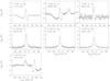Fig. 1 Spectra of H$\begin{array}{c}\mathrm{16}\\ \mathrm{2}\end{array}$O lines toward the high-mass star-forming region AFGL 2591. Dashed red lines are drawn at the source velocity VLSR = −5.5 km s-1. Green lines present the outflow components. We note that the H2O 212−101 and 221−212 lines occur in opposite sidebands of the same spectrum, causing the features near 20 km s-1.

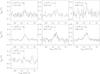Fig. 2 Spectra of H$\begin{array}{c}\mathrm{17}\\ \mathrm{2}\end{array}$O and H$\begin{array}{c}\mathrm{18}\\ \mathrm{2}\end{array}$O lines toward the high-mass star-forming region AFGL 2591. Dashed lines are drawn at the source velocity VLSR = −5.5 km s-1.

AFGL 2591 has been observed in water lines over a range of excitation conditions. Helmich et al. (1996) found more than 30 lines within the bending vibration of water between 5.5 and 6.6 μm using ISO-SWS. No lines of H$\begin{array}{c}\mathrm{18}\\ \mathrm{2}\end{array}$O or vibrationally-excited H₂O were seen. The ISO data indicate a high excitation temperature (>200 K) and a high abundance (~2−6 × 10^-5). Boonman et al. (2003) observed gas-phase H₂O lines between 5 and 540 μm with ISO and SWAS. They found that ice evaporation in the warm inner envelope and freeze-out in the cold outer part together with pure gas-phase chemistry reproduces the H₂O observations. However, these conclusions were based on spectrally unresolved data that could not separate envelope and outflow. van der Tak et al. (2006) and Wang et al. (2012) presented ground-based observations of H$\begin{array}{c}\mathrm{18}\\ \mathrm{2}\end{array}$O toward AFGL 2591 with the Plateau de Bure Interferometer, which have high resolution but are limited to a single line. These data confirm the abundance jump inferred from the ISO/SWAS data, and suggest the presence of a circumstellar disk.

This paper uses Herschel/HIFI observations of water lines toward AFGL 2591 to learn about physical processes in this region and measure the abundance of water in its various physical components as a step towards understanding the process of high-mass star formation. With its much higher spatial and spectral resolution and higher sensitivity than previous space missions, Herschel/HIFI is able to resolve the line profiles and detect isotopic lines, providing essential information on the physical and chemical structure of the region.

Our observations of AFGL 2591 are summarized in Sect. 2. In Sect. 3 we show the observational results and simple analysis. Section 4 presents the analysis of physical conditions using observational data and radiative transfer modeling. Finally, we discuss our results in Sect. 5.

2. Observations

AFGL 2591 was observed with the Heterodyne Instrument for the Far-Infrared (HIFI; de Graauw et al. 2010) onboard ESA’s Herschel Space Observatory (Pilbratt et al. 2010). These observations were conducted between March and June 2010, using the dual beam switch (DBS) mode as part of the guaranteed time key program Water In Star-forming regions with Herschel (WISH; van Dishoeck et al. 2011). The coordinates of the observed position in AFGL 2591 are 20^h29^m24 $\mathit{.}{}^{\mathrm{s}}$87 and +40°11′19.5″ (J2000).

Data were taken simultaneously in horizontal and vertical polarizations using both the correlator-based high-resolution spectrometer (HRS) and the acousto-optical wide-band spectrometer (WBS) with a 1.1 MHz resolution. We used the double beam switch observing mode with a throw of 3′. HIFI receivers are double sideband with a sideband ratio close to unity. Currently, the flux scale accuracy is estimated to be about 10% for bands 1 and 2, 15% for bands 3 and 4, and 20% in bands 6 and 7 (Roelfsema et al. 2012). We show the HRS spectra in Figs. 1 and 2, with the exception of the p-H₂O 1₁₁−0₀₀, o-H₂O 2₁₂−1₀₁, o-H₂O 2₂₁−2₁₂, and o-H$\begin{array}{c}\mathrm{17}\\ \mathrm{2}\end{array}$O 2₁₂−1₀₁ lines, for which WBS spectra were used since the velocity range covered by the HRS was insufficient.

AFGL 2591 was also mapped with HIFI in OTF mode in the o-H₂O 1₁₀−1₀₁, p-H₂O 1₁₁−0₀₀, and p-H₂O 2₀₂−1₁₁ lines. These observations were carried out between November and December 2010. We have taken the o-H₂O 1₁₀−1₀₁ and o-H$\begin{array}{c}\mathrm{18}\\ \mathrm{2}\end{array}$O 1₁₀−1₀₁ lines from the central positions of the maps since we do not have data for these two lines using the double beam switch observing mode. A full analysis of these maps will be presented elsewhere.

The frequencies, energy of the upper levels, system temperatures, integration times, the beam size and efficiency, rms noise level at a given spectral resolution for each of the lines are provided in Table 1. The calibration of the data was performed in the Herschel interactive processing environment (HIPE; Ott 2010) version 8.0. The resulting Level 2 double sideband (DSB) spectra were exported to the FITS format for a subsequent data reduction and analysis using the IRAM GILDAS¹ package. These lines are not expected to be polarized, thus, after inspection, data from the two polarizations were averaged together.

3. Results

The HIFI spectra of AFGL 2591 show strong emission and absorption by H₂O (Fig. 1), and weaker emission in H$\begin{array}{c}\mathrm{18}\\ \mathrm{2}\end{array}$O and H$\begin{array}{c}\mathrm{17}\\ \mathrm{2}\end{array}$O lines (Fig. 2). The line profiles differ considerably between the ground-state levels of H₂O, its excited levels, and its isotopologs.

The ground-state lines of the main isotopologue (p-H₂O 1₁₁−0₀₀, o-H₂O 2₁₂−1₀₁, o-H₂O 1₁₀−1₀₁) show a mix of emission and absorption, as found before for DR21 (van der Tak et al. 2010) and W3 IRS5 (Chavarría et al 2010). First, all three lines show an emission feature of the source at V_LSR = −3 km s^-1, somewhat red-shifted with respect to the V_LSR of the source at V_LSR = −5.5 km s^-1 (van der Tak et al. 1999). The emission feature seems to be related to an expansion of the outer envelope. The expansion is probably powered by outflows which are known to exist in AFGL 2591 (Lada et al. 1984). The blue side of the emission is smooth because of the outflow, but the red side is sharply truncated because of absorption by a foreground cloud at ~0 km s^-1.

Second, a broad and asymmetric absorption component occurs near V_LSR = −10 km s^-1 which from its shape has a likely origin in a wind. This broad absorption component is only detected in the p-H₂O 1₁₁−0₀₀ and o-H₂O 2₁₂−1₀₁ lines. We probably do not see it in the o-H₂O 1₁₀−1₀₁ line because the signal-to-noise ratio on the continuum is not high enough.

Third, the ground-state H₂O line profiles show evidence for two foreground clouds. The narrow absorption component around V_LSR = 0 km s^-1 is detected in all three lines, and corresponds to a cloud known from ground-based observations (van der Tak et al. 1999). A second, weaker absorption feature near V_LSR = 13 km s^-1 is only seen in the p-H₂O 1₁₁−0₀₀ line. The continuum at o-H₂O 1₁₀−1₀₁ line is presumably too weak to see this feature, and the o-H₂O 2₁₂−1₀₁ spectrum is blended with the o-H₂O 2₂₁−2₁₂ line. This cloud is not known from ground-based observations, and is also seen in HF observations (Emprechtinger et al. 2012) but not in CO observations by Herschel/HIFI of this source (van der Wiel et al. 2013), so it is probably a diffuse cloud.

The excited-state lines of H₂O (p-H₂O 2₀₂−1₁₁, p-H₂O 2₁₁−2₀₂, and o-H₂O 3₁₂−3₀₃) appear purely in emission and show two velocity components. The components have Gaussian shapes, one being wider (FWHM = 11−12 km s^-1) than the other (FWHM = 3−4 km s^-1). Studies of low-mass protostars from the WISH program (Kristensen et al. 2010, 2012) refer to these components as the broad and narrow components, but we will call them the outflow and envelope components, after their likely physical origin. We assume that the broad component is due to the high-velocity outflow associated with the protostar seen in absorption in p-H₂O 1₁₁−0₀₀ and o-H₂O 2₁₂−1₀₁ lines, even though it covers a somewhat smaller velocity range. The narrow component is potentially associated with the protostellar envelope.

The lines of H$\begin{array}{c}\mathrm{18}\\ \mathrm{2}\end{array}$O and H$\begin{array}{c}\mathrm{17}\\ \mathrm{2}\end{array}$O appear purely in emission and are dominated by the envelope, centered around V_LSR = −5 km s^-1. In addition, the H$\begin{array}{c}\mathrm{18}\\ \mathrm{2}\end{array}$O lines around 1 THz may show a broadening due to a weak outflow component. Likewise, the high-frequency o-H$\begin{array}{c}\mathrm{17}\\ \mathrm{2}\end{array}$O 1₁₀−1₀₁ line appears to be broader than the other two H$\begin{array}{c}\mathrm{17}\\ \mathrm{2}\end{array}$O lines.

We extracted line parameters from the observed profiles by fitting Gaussians; Table 2 gives the results for the emission lines and Table 3 for the absorption lines. For the emission features, we fitted the p-H₂O 2₀₂−1₁₁, p-H₂O 2₁₁−2₀₂, and o-H₂O 3₁₂−3₀₃ line profiles assuming two velocity components, while the other emission lines are fitted as one velocity component. The H$\begin{array}{c}\mathrm{18}\\ \mathrm{2}\end{array}$O lines appear broader than the narrow emission components seen in H₂O (see Table 2), so that the profiles are probably a mixture of envelope and outflow emission seen at limited signal-to-noise ratio. The o-H$\begin{array}{c}\mathrm{17}\\ \mathrm{2}\end{array}$O 1₁₀−1₀₁ might show two components but the signal-to-noise ratio is not good enough so that we assume that this line has one component.

4. Analysis

4.1. Absorption components

The ground-state lines of the main isotopologue (p-H₂O 1₁₁−0₀₀, o-H₂O 2₁₂−1₀₁, o-H₂O 1₁₀−1₀₁) show three absorption components: 1) the broad V_LSR = −10 km s^-1 component due to the molecular outflow; 2) the narrow V_LSR = 0 km s^-1 component due to the known foreground cloud; and 3) the narrow V_LSR = 13 km s^-1 component due to a new diffuse foreground cloud. We derived the optical depth in these three components using the expression 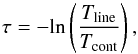$\mathit{\tau }\mathrm{=}\mathrm{-}\ln \left(\frac{{\mathit{T}}_{\mathrm{line}}}{{\mathit{T}}_{\mathrm{cont}}}\right)\mathit{,}$(1)where T_cont is the single side band (SSB) continuum intensity. This expression assumes that the sideband gain ratio is unity and that the continuum is completely covered by the absorbing layer. We applied a linear baseline fit in the vicinity of the absorption line to derive the continuum intensity at the absorption peak. Deriving the optical depth from the line-to-continuum ratio is based on the assumption that the excitation temperature is negligible with respect to the continuum temperature.

In the following analysis we assume that all water molecules are in the ortho and para ground states, so that the velocity integrated absorption is related to the molecular column density by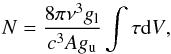$\mathit{N}\mathrm{=}\frac{\mathrm{8}\mathit{\pi }{\mathit{\nu }}^{\mathrm{3}}{\mathit{g}}_{\mathrm{l}}}{{\mathit{c}}^{\mathrm{3}}\mathit{A}{\mathit{g}}_{\mathrm{u}}}\mathrm{\int }\mathit{\tau }\mathrm{d}\mathit{V}\mathit{,}$(2)where N is the column density, ν the frequency, c the speed of light, and τ is the optical depth. A stands for the Einstein-A coefficient and g_l and g_u are the degeneracy of the lower and the upper level of the transition. Subsequently, we integrated over the velocity ranges given in Table 3 to determine the column density for each component. The derived column densities and the optical depth of the three components are listed also in Table 3. For the velocity range from −24 km s^-1 to −5.5 km s^-1, the column density is ~2−7 × 10¹³ cm^-2 and the optical depth is ~0.5−1. On the other hand, the column density is ~1−4 × 10¹³ cm^-2 and the averaged optical depth is ~1.6−2 for the velocity range from −2 km s^-1 to 1.5 km s^-1.

More information about the physical conditions in the foreground clouds comes from the ortho-to-para ratio of H₂O. If this ratio is thermalized, it should rise from ~1 at low temperatures (~15 K) to ~3 at high temperatures (>40 K) as shown by Mumma et al. (1987). Since we have data for ortho- and para-H₂O, we can determine the ortho/para (o/p) ratio, although the dynamic range of the absorption data is limited by the signal-to-noise ratio on one hand and by saturation on the other.

For narrow component, we determine the o/p ratio using the ground state of the o-H₂O 1₁₀−1₀₁ and the p-H₂O 1₁₁−0₀₀ lines and we find a lower o/p ratio of ~1.9 ± 0.4 in the narrow component, suggesting a lower temperature for the foreground cloud. On the other hand, for the broad component we do not see it in the o-H₂O 1₁₀−1₀₁ line so we used the second ground state ortho-H₂O line, o-H₂O 2₁₂−1₀₁ transition at 1670 GHz. The o/p ratio of the broad component is around three (~3.5 ± 1.0), which is reasonable because the gas in the outflow is probably warm as it is heated by shocks.

Similar results have been found for diffuse absorbing clouds toward continuum sources in the Galactic plane (Flagey et al. 2013). Their presented water o/p ratios were consistent with the high-temperature limit value of 3, with lower values for the clouds with the highest column densities. Presumably interstellar UV radiation does not fully penetrate those clouds, so that photo-electric heating of the gas is less efficient. Indeed, the total (ortho + para) H₂O column densities of the foreground clouds of AFGL 2591 are as high as ~5 × 10¹³ cm^-2 assuming an o/p ratio of 3, similar to the values found for the clouds toward NGC 6334 I, which also have a similar o/p ratio of H₂O (Emprechtinger et al. 2010).

4.2. Emission components

To estimate the column densities and rotation temperatures of water in the envelope and outflow of AFGL 2591, we construct rotation diagrams for the H$\begin{array}{c}\mathrm{17}\\ \mathrm{2}\end{array}$O and H$\begin{array}{c}\mathrm{18}\\ \mathrm{2}\end{array}$O lines for the envelope and for the broad component of the p-H₂O 2₀₂−1₁₁, p-H₂O 2₁₁−2₀₂, and o-H₂O 3₁₂−3₀₃ lines for the outflow. We assume an ${\mathrm{16}}^{}$O/${\mathrm{18}}^{}$O ratio of 550 and an ${\mathrm{18}}^{}$O/${\mathrm{17}}^{}$O ratio of 4 (Wilson & Rood 1994), and that the H$\begin{array}{c}\mathrm{17}\\ \mathrm{2}\end{array}$O and H$\begin{array}{c}\mathrm{18}\\ \mathrm{2}\end{array}$O lines have the same excitation temperature.

First, we assume that (1) the lines are optically thin; (2) the emission fills the telescope beam; and (3) all level populations can be characterized by a single excitation temperature T_rot and use following equations. The column densities of the molecules in the upper level N_u are related to the measured integrated intensities, ^∫T_mbdV (Linke et al. 1979; Blake et al. 1984, 1987; Helmich et al. 1994) by 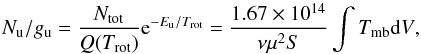${\mathit{N}}_{\mathrm{u}}\mathit{/}{\mathit{g}}_{\mathrm{u}}\mathrm{=}\frac{{\mathit{N}}_{\mathrm{tot}}}{\mathit{Q}\mathrm{\left(}{\mathit{T}}_{\mathrm{rot}}\mathrm{\right)}}{\mathrm{e}}^{\mathrm{-}{\mathit{E}}_{\mathrm{u}}\mathit{/}{\mathit{T}}_{\mathrm{rot}}}\mathrm{=}\frac{\mathrm{1.67}\mathrm{\times }{\mathrm{10}}^{\mathrm{14}}}{\mathit{\nu }{\mathit{\mu }}^{\mathrm{2}}\mathit{S}}\mathrm{\int }{\mathit{T}}_{\mathrm{mb}}\mathrm{d}\mathit{V}\mathit{,}$(3)where μ is the permanent dipole moment, N_tot is the total column density, Q(T_rot) is the partition function for the rotation temperature T_rot, and S is the line strength value. Thus, a logarithmic plot of the quantity on the right-hand side of equation as a function of E_u provides a straight line with slope 1 /T_rot and intercept N_tot/Q(T_rot).

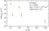Fig. 3 Rotation diagram for the H$\begin{array}{c}\mathrm{18}\\ \mathrm{2}\end{array}$O and H$\begin{array}{c}\mathrm{17}\\ \mathrm{2}\end{array}$O emission components (envelope). Red open circles are the data observed with Herschel/HIFI. The green crosses represent the best-fit model from the population diagram analysis.

To test our assumption of low optical depth in the above analysis, we carry out a simple estimate of the line optical depths comparing the observed H$\begin{array}{c}\mathrm{16}\\ \mathrm{2}\end{array}$O-to-H$\begin{array}{c}\mathrm{18}\\ \mathrm{2}\end{array}$O and H$\begin{array}{c}\mathrm{18}\\ \mathrm{2}\end{array}$O-to-H$\begin{array}{c}\mathrm{17}\\ \mathrm{2}\end{array}$O line ratios to the isotopic ratios, based on the assumption that the excitation temperatures of the corresponding transitions is the same across isotopologues. The measured peak intensity ratios of the p-H$\begin{array}{c}\mathrm{16}\\ \mathrm{2}\end{array}$O 2₀₂−1₁₁-to-p-H$\begin{array}{c}\mathrm{18}\\ \mathrm{2}\end{array}$O 2₀₂−1₁₁ and o-H$\begin{array}{c}\mathrm{16}\\ \mathrm{2}\end{array}$O 3₁₂−3₀₃-to-p-H$\begin{array}{c}\mathrm{18}\\ \mathrm{2}\end{array}$O 3₁₂−3₀₃ lines are 14 and 10, respectively, which is well below the isotopic ratio and indicates an optical depth of 3.6−3.9 for H$\begin{array}{c}\mathrm{16}\\ \mathrm{2}\end{array}$O. In contrast, our observed p-H$\begin{array}{c}\mathrm{18}\\ \mathrm{2}\end{array}$O 1₁₁−0₀₀-to-p-H$\begin{array}{c}\mathrm{17}\\ \mathrm{2}\end{array}$O 1₁₁−0₀₀ line ratio is ~2, close to the isotopic ratio, which means that the optical depth of the H$\begin{array}{c}\mathrm{18}\\ \mathrm{2}\end{array}$O lines is ≲1.

We now construct rotation diagrams which take into account the effect of optical depth. We define the optical depth correction factor C_τ (= τ/ (1−e^{− τ})). If the source does not fill the beam, then the correct upper level column density is greater than that obtained assuming the beam to be filled by a factor equal to the beam dilution f( = ΔΩ_a/ ΔΩ_s), with Ω_s the size of the emission region and Ω_a the size of the telescope beam. The equation mentioned for the rotation diagram method as Eq. (3) can be modified to include the effect of optical depth τ through the factor C_τ and beam dilution f (Goldsmith & Langer 1999): 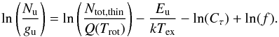$\ln \left(\frac{{\mathit{N}}_{\mathrm{u}}}{{\mathit{g}}_{\mathrm{u}}}\right)\mathrm{=}\ln \left(\frac{{\mathit{N}}_{\mathrm{tot}\mathit{,}\mathrm{thin}}}{\mathit{Q}\mathrm{\left(}{\mathit{T}}_{\mathrm{rot}}\mathrm{\right)}}\right)\mathrm{-}\frac{{\mathit{E}}_{\mathrm{u}}}{\mathit{k}{\mathit{T}}_{\mathrm{ex}}}\mathrm{-}\ln \mathrm{\left(}{\mathit{C}}_{\mathit{\tau }}\mathrm{\right)}\mathrm{+}\ln \mathrm{\left(}\mathit{f}\mathrm{\right)}\mathit{.}$(4)According to Eq. (4), for a given upper level, N_u can be evaluated from a set of N_tot,thin, T_ex, f and C_τ. Since C_τ is a function of N_tot,thin and T_ex, the independent parameters are therefore N_tot,thin, T_ex and f, for which we solve self-consistently. A χ² minimization gives best-fit values of N_tot,thin, T_ex, and source sizes. In Figs. 3 and 4, rotation diagrams for water molecules in AFGL 2591 are presented. Red open circles are the data observed with Herschel/HIFI and the green crosses represent the best-fit model from population diagram analysis (using Eq. (4)).

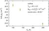Fig. 4 Rotation diagram for the broad emission components seen in p-H2O 202−111, p-H2O 211−202, and o-H2O 312−303 (outflow). Red open circles are the data observed with Herschel/HIFI. The green crosses represent the best-fit model from the population diagram analysis.

Figure 3 shows the rotation diagram for H$\begin{array}{c}\mathrm{18}\\ \mathrm{2}\end{array}$O and H$\begin{array}{c}\mathrm{17}\\ \mathrm{2}\end{array}$O, which is associated with the envelope. We construct rotation diagram for the envelope using five H$\begin{array}{c}\mathrm{18}\\ \mathrm{2}\end{array}$O and H$\begin{array}{c}\mathrm{17}\\ \mathrm{2}\end{array}$O emission lines because we do not detect the o-H$\begin{array}{c}\mathrm{18}\\ \mathrm{2}\end{array}$O 1₁₀−1₀₁ line and p-H$\begin{array}{c}\mathrm{18}\\ \mathrm{2}\end{array}$O 1₁₁−0₀₀ line and p-H$\begin{array}{c}\mathrm{17}\\ \mathrm{2}\end{array}$O 1₁₁−0₀₀ line have the same energy of the upper level so we use the p-H$\begin{array}{c}\mathrm{17}\\ \mathrm{2}\end{array}$O 1₁₁−0₀₀ line which is optically thin. The excitation temperature is estimated to be 42 ± 7 K with column density of (1.7 ± 0.7) × 10¹⁴ cm^-2 distributed over a ~4″ region. Line opacities of all the transitions used are estimated to be less than 14, which are consistent with those derived from the observed H$\begin{array}{c}\mathrm{16}\\ \mathrm{2}\end{array}$O-to-H$\begin{array}{c}\mathrm{18}\\ \mathrm{2}\end{array}$O line ratios to the isotopic ratios.

Figure 4 presents the same analysis for the broad components seen in p-H₂O 2₀₂−1₁₁, p-H₂O 2₁₁−2₀₂, and o-H₂O 3₁₂−3₀₃. The broad component is likely related to the outflow, for which we find an excitation temperature of 45 ± 4 K, a column density of (4.2 ± 1.0) × 10¹³ cm^-2, a source size of ~30″ and line opacities of the three H₂O transitions (broad components) used of <0.03.

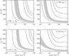Fig. 5 Excitation temperature of p-H$\begin{array}{c}\mathrm{18}\\ \mathrm{2}\end{array}$O 111−000, p-H$\begin{array}{c}\mathrm{18}\\ \mathrm{2}\end{array}$O 202−111 for the envelope (upper) and the p-H2O 211−202, p-H2O 202−111 for the outflow (lower) assuming H2O column densities of N(H2O) = 1 × 1014 cm-2 and N(H2O) = 5 × 1013 cm-2 and source sizes of 4″ and 30″ for the envelope and the outflow, respectively as a function of kinetic temperature and H2 density calculated with RADEX (Non-LTE, large velocity gradient code). The gray areas indicate the derived Tex of envelope and outflow from the LTE rotation diagram analysis.

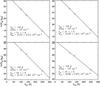Fig. 6 Examples of rotation diagram for the p-H2O 202−111, p-H2O 211−202, and o-H2O 312−303 emission lines originating in the outflow at a given kinetic temperature of Tkin = 100 K from the RADEX calculations (non-LTE analysis). Open circles are the data from the non-LTE models. The overplotted line corresponds to a linear fit to the rotational diagram.

4.3. Non-LTE calculations

We carried out non-local thermodynamic equilibrium (LTE) models of H₂O using the RADEX code (van der Tak et al. 2007) and state-of-the-art quantum mechanical collision rates of para and ortho H₂O with para and ortho H₂ (Daniel et al. 2011) as provided at the LAMDA database (Schöier et al. 2005). The same collision data are used for all isotopologs. To constrain the H₂O excitation, we generated a grid of models with values of T_kin between 10 and 1000 K, values of n(H₂) from 10³ to 10⁹ cm^-3, and fixed the background radiation temperature at 2.73 K. The line width was fixed at 3 km s^-1 for the envelope and 10.5 km s^-1 for the outflow, and we applied a molecular column density of N(H₂O) = 1 × 10¹⁴ cm^-2 and N(H₂O) = 5 × 10¹³ cm^-2 for the envelope and the outflow, respectively. These molecular column densities are derived by the rotation diagram method (LTE) assuming source sizes of 4″ and 30″.

In the comparison with data, we first focus on the p-H$\begin{array}{c}\mathrm{18}\\ \mathrm{2}\end{array}$O 1₁₁−0₀₀ and p-H$\begin{array}{c}\mathrm{18}\\ \mathrm{2}\end{array}$O 2₀₂−1₁₁ lines for the envelope, which lie close in frequency, so that the effects of beam filling cancel out to first order. For the outflow, we use the p-H₂O 2₁₁−2₀₂ and p-H₂O 2₀₂−1₁₁ lines, based on the calculations of the p-H₂O 2₁₁−2₀₂/p-H₂O 2₀₂−1₁₁ line ratio, which traces both the gas temperature and density (Fig. A.1).

Figure 5 presents the calculated excitation temperatures of the p-H$\begin{array}{c}\mathrm{18}\\ \mathrm{2}\end{array}$O 1₁₁−0₀₀ and p-H$\begin{array}{c}\mathrm{18}\\ \mathrm{2}\end{array}$O 2₀₂−1₁₁ lines for the envelope (upper) and of the p-H₂O 2₁₁−2₀₂ and p-H₂O 2₀₂−1₁₁ lines for the outflow (lower), as a function of gas density and kinetic temperature. The calculations show that the derived range of excitation temperatures for the envelope (gray area in upper panels) based on the rotation diagram method (LTE) indicates a gas density of 7 × 10⁶−10⁸ cm^-3 and a kinetic temperature of ~60−230 K indicating subthermal excitation. On the other hand, the models indicate that a gas density of ~10⁷−10⁸ cm^-3 and a kinetic temperature of ~70−90 K reproduce the observations of the outflow (gray area in lower panels).

To compare LTE and non-LTE calculations, we construct the rotation diagrams for the broad components of the p-H₂O 2₀₂−1₁₁, p-H₂O 2₁₁−2₀₂, and o-H₂O 3₁₂−3₀₃ lines using the RADEX calculation as data points at different kinetic temperatures, T_kin, and densities, n(H₂). We apply a molecular column density of N(H₂O) = 5 × 10¹³ cm^-2 and a line width of 10.5 km s^-1. Figure 6 presents the rotation diagrams for the broad components of the three excited-state lines of H₂O assuming a kinetic temperature of T_kin = 100 K as examples. Open circles are the data from the RADEX calculations. The overplotted line represents a linear fit to the rotational diagram. The rotation temperatures, T_rot, are below the input kinetic temperature of T_kin = 100 K. At higher H₂ density the rotation temperature is higher than at low H₂ density but our results show that the rotation temperature is well below the kinetic temperature, even at n(H₂) = 10⁸ cm^-3. Higher densities are implausible for AFGL 2591 at the spatial scales probed by our data.

5. Discussion

We estimate the H₂O abundance in the various physical components of AFGL 2591 (Table 4) assuming a constant abundance for the protostellar envelope. First, van der Wiel et al. (2013) presents an absorption feature seen in CO 5–4 and JCMT data of CO 3–2 near 0 km s^-1, which is known to be a foreground component. They derived a column density N(H₂) ≳3 × 10²¹ cm^-2 assuming an abundance of CO/H₂ of 10^-4. Assuming an o/p ratio of 3, we estimate the total (ortho+para) H₂O column density for the 0 km s^-1 foreground component using the p-H₂O 1₁₁−0₀₀ line. We find that the total H₂O column density is ~5.2 × 10¹³ cm^-2. and the abundance of H₂O is ≲1.7 × 10^-8, consistent with ion-molecule chemistry. In addition to the 0 km s^-1 foreground component, there is another weak absorption component at 13 km s^-1, for which van der Wiel et al. (2013) obtained limits on the H₂ column density. As an upper limit, they estimated N(H₂) ≲6 × 10²¹ cm^-2 based on their ¹³CO 1–0 spectrum. In addition, they used the HF 1–0 spectrum presented by Emprechtinger et al. (2012) to obtain a lower limit for the column density of the 13 km s^-1 foreground component. They found that N(H₂) ≳8 × 10²⁰ cm^-2 assuming HF/H₂ = 3.6 × 10^-8. We estimate the H₂O column density of N(H₂O) = 1.6 × 10¹² cm^-2 using the p-H₂O 1₁₁−0₀₀ line under the assumptions that an o/p ratio is 3, so that the H₂O abundance in this component is ~10^-9. This lower abundance compared with the 0 km s^-1 component is consistent with enhanced photodissociation in diffuse gas.

In order to derive the H₂O abundance in the outflow and envelope components, we use two methods to estimate the H₂ column density. We adopt the H₂O column densities of ~1.7 × 10¹⁴ cm^-2 for the envelope and ~4.2 × 10¹³ cm^-2 for the outflow, in source sizes of 4″ and 30″, respectively, based on LTE calculations. Mitchell et al. (1989) detected CO and ¹³CO rovibrational absorption lines near 4.7 μm and found a cold (~38 K) and a hot (~1000 K) component in the quiescent gas centered around −5 km s^-1, and a blueshifted warm (~200 K) component. The cold component is likely the outer envelope of AFGL 2591, while the hot gas is near the infrared source and is heated by its luminosity. Despite their different temperatures, the CO column densities of the three components are all in the range 5−7 × 10¹⁸ cm^-2. We use the column density from the cold gas for the envelope, and that of the blueshifted warm gas for the outflow, and derive the column density of H₂ using a ratio N(${\mathrm{12}}^{}$CO)/N(H₂) = 10^-4. We find that the abundance of H₂O is 2.4 × 10^-9 for the envelope and 6.4 × 10^-10 for the outflow.

As a second method, we estimate N(H₂) from submillimeter observations. San José-García et al. (2013) presented Herschel/HIFI observations of high-J CO and isotopologues from low-to high-mass star-forming regions. They estimated a H₂ column density for AFGL 2591 of 2.7 × 10²² cm^-2 in a ~20″ beam using C¹⁸O J = 9–8 for an excitation temperature of 75 K. Using this column density of H₂, we find that the abundance of H₂O is 6.3 × 10^-9 for the envelope in a source size of 4″. van der Wiel et al. (2013) also estimated the column density of H₂ for the envelope and outflow regions using Herschel/HIFI data of CO and they found that the column density of H₂ is ~10²² cm^-2 and 1.5 × 10²² cm^-2 for the envelope and outflow, respectively. Using these numbers, the abundance of H₂O is 1.7 × 10^-8 for the envelope and 2.8 × 10^-9 for the outflow. Since our derived H₂O source size of 4″ is between the beam sizes of the infrared and submillimeter estimates for N(H₂), the most likely value for the H₂O abundance is between the above estimates. Since the outflow gas is more extended, the abundance estimate from the submillimeter CO data is probably the best.

In summary, our Herschel/HIFI observations indicate water abundances of ~2 × 10^-9−2 × 10^-8 and a kinetic temperature of ~60−230 K in the envelope. These abundances are much lower than found from infrared (ISO) data (Sect. 1), which indicates that our observed emission comes mostly from the cold outer envelope. Indeed, our derived water abundance is similar to the values of 5 × 10^-10 to 4 × 10^-8 found for the outer envelopes of other high-mass protostars (van der Tak et al. 2010; Chavarría et al. 2010; Marseille et al. 2010; Herpin et al. 2012), and also for low-mass protostellar envelopes (Kristensen et al. 2012). In contrast, the infrared absorption data are mostly sensitive to the warm inner envelope, and we expect this gas to emit primarily in the PACS lines rather than the HIFI lines. Indeed, using the Herschel/PACS instrument, Karska et al. (2014) probe a warm water component which is similar to the gas seen with ISO.

For the outflow, we find a water abundance of ~6 × 10^-10−3 × 10^-9 and a kinetic temperature of ~70−90 K. Despite the similar temperatures, the H₂O abundance in the outflow is a factor of 10 lower than in the AFGL 2591 envelope and also lower than found for other outflows, both from high-mass (van der Tak et al. 2010; Emprechtinger et al. 2013) and low-mass (Bjerkeli et al. 2012) protostars. The abundance estimate is uncertain through the adopted source size, but this effect is probably small as seen from a comparison of the column densities measured in absorption (Table 3) and emission (Table 4). The absorbing column is almost twice the emitting column, which suggests a source size of ~20″ rather than ~30″, assuming that the features arise in the same gas. The corresponding effect on the H₂O column density and abundance is only a factor of 2. However, the effect is probably smaller because the emission occurs over a smaller velocity range (from −15 to −5 km s^-1) than the absorption (from −24 to −5.5 km s^-1) which suggests that the features do not arise in the same gas. More likely, the water in the outflow lobes is affected by dissociating UV radiation, which also means that the H$\begin{array}{c}\mathrm{18}\\ \mathrm{2}\end{array}$O lines are dominated by shocks at the interface between the jets and the envelope.

6. Conclusions

• 1.

  We present 14 rotational transitions of H₂O, H$\begin{array}{c}\mathrm{17}\\ \mathrm{2}\end{array}$O, and H$\begin{array}{c}\mathrm{18}\\ \mathrm{2}\end{array}$O toward the massive star-forming region AFGL 2591.

• 2.

  We find redshifted water absorption from cold foreground clouds and blueshifted absorption from the outflow. Similar line features are found in W3 IRS5 (Chavarría et al. 2010) and DR21 (van der Tak et al. 2010)

• 3.

  We derived the o/p ratio using the ground-state lines of the main isotopologue and found that the o/p ratio is ~2 in the cold foreground cloud, while the o/p ratio is ~3 in the warm protostellar envelope. Similar results are found toward Sgr B2(M) (Lis et al. 2010) and NGC 6334 I (Emprechtinger et al. 2010). The inferred water abundances in the foreground clouds are consistent with ion-molecule chemistry.

• 4.

  Radiative transfer models indicate that the envelope of AFGL 2591 is warm (T_kin ~ 60−230 K). However, the low derived H₂O abundance (~2 × 10^-9−2 × 10^-8) suggests that the H₂O line emission is dominated by the cold outer envelope where freeze-out of water onto dust grains is important. This apparent contradiction suggests that the water abundance in the protostellar envelope varies with radius.

• 5.

  The water abundance in the outflow is ~10× lower than in the envelope and in the outflows of other high- and low-mass protostars. Part of this difference may be due to beam size effect, but another possibility is the effect of dissociating UV radiation (van Dishoeck et al. 2013). Compared to the envelope, the outflow lobes have a lower extinction, which leads to a higher UV radiation field and thus more rapid photodissociation. However, why this outflow has a lower H₂O abundance than those of other high-mass protostars is unclear. Models of UV-irradiated shocks are being developed to interpret the observed water abundances in protostellar outflows (Kaufman, priv. comm.).

The environment of AFGL 2591 has been the target of many observations from the ground and from space, but the Herschel/HIFI H₂O observations show the kinematics of this source (outflow, expanding envelope, foreground cloud) in more detail than any previous study. This opportunity will be further explored with detailed radiative transfer models (Hogerheijde & van der Tak 2000) in a future paper, where we will estimate H₂O abundance profiles for a sample of high-mass protostellar envelopes.

Acknowledgments

The authors thank the referee for the careful and detailed report that helped to improve the paper. We also thank the editor, Malcolm Walmsley, for additional helpful comments. We thank Kuo-Song Wang for the use of his population diagram code, and Asunción Fuente and Timea Csengeri for useful comments on our manuscript. HIFI has been designed and built by a consortium of institutes and university departments from across Europe, Canada, and the US under the leadership of SRON Netherlands Institute for Space Research, Groningen, The Netherlands, with major contributions from Germany, France and the US. Consortium members are: Canada: CSA, U. Waterloo; France: CESR, LAB, LERMA, IRAM; Germany: KOSMA, MPIfR, MPS; Ireland, NUI Maynooth; Italy: ASI, IFSI-INAF, Arcetri-INAF; Netherlands: SRON, TUD; Poland: CAMK, CBK; Spain: Observatorio Astronómico Nacional (IGN), Centro de Astrobiología (CSIC-INTA); Sweden: Chalmers University of Technology – MC2, RSS & GARD, Onsala Space Observatory, Swedish National Space Board, Stockholm University – Stockholm Observatory; Switzerland: ETH Zürich, FHNW; USA: Caltech, JPL, NHSC.

References

Appendix A: RADEX line ratio plot

In Sects. 4.3 we calculate the line ratios of p-H₂O 2₁₁−2₀₂ and p-H₂O 2₀₂−1₁₁ using the non-LTE code RADEX (van der Tak et al. 2007). Figure A.1 shows the p-H₂O 2₁₁−2₀₂ and p-H₂O 2₀₂−1₁₁ line intensity ratio for kinetic temperatures between 20 K and 300 K and H₂ densities between 10³ cm^-3 and 5 × 10⁸ cm^-3.

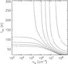Fig. A.1 Line ratios of p-H2O 211−202 and p-H2O 202−111 as a function of kinetic temperature and H2 density.

All Tables

All Figures

	Fig. 1 Spectra of H$\begin{array}{c}\mathrm{16}\\ \mathrm{2}\end{array}$O lines toward the high-mass star-forming region AFGL 2591. Dashed red lines are drawn at the source velocity VLSR = −5.5 km s-1. Green lines present the outflow components. We note that the H2O 212−101 and 221−212 lines occur in opposite sidebands of the same spectrum, causing the features near 20 km s-1.
In the text

	Fig. 2 Spectra of H$\begin{array}{c}\mathrm{17}\\ \mathrm{2}\end{array}$O and H$\begin{array}{c}\mathrm{18}\\ \mathrm{2}\end{array}$O lines toward the high-mass star-forming region AFGL 2591. Dashed lines are drawn at the source velocity VLSR = −5.5 km s-1.
In the text

	Fig. 3 Rotation diagram for the H$\begin{array}{c}\mathrm{18}\\ \mathrm{2}\end{array}$O and H$\begin{array}{c}\mathrm{17}\\ \mathrm{2}\end{array}$O emission components (envelope). Red open circles are the data observed with Herschel/HIFI. The green crosses represent the best-fit model from the population diagram analysis.
In the text

	Fig. 4 Rotation diagram for the broad emission components seen in p-H2O 202−111, p-H2O 211−202, and o-H2O 312−303 (outflow). Red open circles are the data observed with Herschel/HIFI. The green crosses represent the best-fit model from the population diagram analysis.
In the text

Fig. 5 Excitation temperature of p-H$\begin{array}{c}\mathrm{18}\\ \mathrm{2}\end{array}$O 111−000, p-H$\begin{array}{c}\mathrm{18}\\ \mathrm{2}\end{array}$O 202−111 for the envelope (upper) and the p-H2O 211−202, p-H2O 202−111 for the outflow (lower) assuming H2O column densities of N(H2O) = 1 × 1014 cm-2 and N(H2O) = 5 × 1013 cm-2 and source sizes of 4″ and 30″ for the envelope and the outflow, respectively as a function of kinetic temperature and H2 density calculated with RADEX (Non-LTE, large velocity gradient code). The gray areas indicate the derived Tex of envelope and outflow from the LTE rotation diagram analysis.

In the text

	Fig. 6 Examples of rotation diagram for the p-H2O 202−111, p-H2O 211−202, and o-H2O 312−303 emission lines originating in the outflow at a given kinetic temperature of Tkin = 100 K from the RADEX calculations (non-LTE analysis). Open circles are the data from the non-LTE models. The overplotted line corresponds to a linear fit to the rotational diagram.
In the text

	Fig. A.1 Line ratios of p-H2O 211−202 and p-H2O 202−111 as a function of kinetic temperature and H2 density.
In the text

References

- Bjerkeli, P., Liseau, R., Larsson, B., et al. 2012, A&A, 546, A29 [NASA ADS] [CrossRef] [EDP Sciences] [Google Scholar]
- Blake, G. A., Sutton, E. C., Masson, C. R., et al. 1984, ApJ, 286, 586 [NASA ADS] [CrossRef] [Google Scholar]
- Blake, G. A., Sutton, E. C., Masson, C. R., & Phillips, T. G. 1987, ApJ, 315, 621 [NASA ADS] [CrossRef] [Google Scholar]
- Boonman, A. M. S., Doty, S. D., van Dishoeck, E. F., et al. 2003, A&A, 406, 937 [NASA ADS] [CrossRef] [EDP Sciences] [Google Scholar]
- Chavarría, L., Herpin, F., Jacq, T., et al. 2010, A&A, 521, L37 [NASA ADS] [CrossRef] [EDP Sciences] [Google Scholar]
- Daniel, F., Dubernet, M.-L., & Grosjean, A. 2011, A&A, 536, A76 [NASA ADS] [CrossRef] [EDP Sciences] [Google Scholar]
- de Graauw, T., Helmich, F. P., Phillips, T. G., et al. 2010, A&A, 518, L6 [NASA ADS] [CrossRef] [EDP Sciences] [Google Scholar]
- Emprechtinger, M., Lis, D. C., Bell, T., et al. 2010, A&A, 521, L28 [NASA ADS] [CrossRef] [EDP Sciences] [Google Scholar]
- Emprechtinger, M., Monje, R. R., van der Tak, F. F. S., et al. 2012, ApJ, 756, 136 [NASA ADS] [CrossRef] [Google Scholar]
- Emprechtinger, M., Lis, D. C., Rolffs, R., et al. 2013, ApJ, 765, 61 [NASA ADS] [CrossRef] [Google Scholar]
- Flagey, N., Goldsmith, P. F., Lis, D. C., et al. 2013, ApJ, 762, 11 [NASA ADS] [CrossRef] [Google Scholar]
- Goldsmith, P. F., & Langer, W. D. 1999, ApJ, 517, 209 [NASA ADS] [CrossRef] [Google Scholar]
- Helmich, F. P., Jansen, D. J., de Graauw, T., Groesbeck, T. D., & van Dishoeck, E. F. 1994, A&A, 283, 626 [NASA ADS] [Google Scholar]
- Helmich, F. P., van Dishoeck, E. F., Black, J. H., et al. 1996, A&A, 315, L173 [NASA ADS] [Google Scholar]
- Herpin, F., Chavarría, L., van der Tak, F., et al. 2012, A&A, 542, A76 [NASA ADS] [CrossRef] [EDP Sciences] [Google Scholar]
- Hogerheijde, M. R., & van der Tak, F. F. S. 2000, A&A, 362, 697 [NASA ADS] [Google Scholar]
- Karska, A., Herpin, F., Bruderer, S., et al. 2014, A&A, 562, A45 [NASA ADS] [CrossRef] [EDP Sciences] [Google Scholar]
- Kristensen, L. E., Visser, R., van Dishoeck, E. F., et al. 2010, A&A, 521, L30 [NASA ADS] [CrossRef] [EDP Sciences] [Google Scholar]
- Kristensen, L. E., van Dishoeck, E. F., Bergin, E. A., et al. 2012, A&A, 542, A8 [NASA ADS] [CrossRef] [EDP Sciences] [Google Scholar]
- Lada, C. J., Thronson, Jr., H. A., Smith, H. A., Schwartz, P. R., & Glaccum, W. 1984, ApJ, 286, 302 [NASA ADS] [CrossRef] [Google Scholar]
- Linke, R. A., Frerking, M. A., & Thaddeus, P. 1979, ApJ, 234, L139 [NASA ADS] [CrossRef] [Google Scholar]
- Lis, D. C., Phillips, T. G., Goldsmith, P. F., et al. 2010, A&A, 521, L26 [NASA ADS] [CrossRef] [EDP Sciences] [Google Scholar]
- Marseille, M. G., van der Tak, F. F. S., Herpin, F., et al. 2010, A&A, 521, L32 [Google Scholar]
- Mitchell, G. F., Curry, C., Maillard, J.-P., & Allen, M. 1989, ApJ, 341, 1020 [NASA ADS] [CrossRef] [Google Scholar]
- Mumma, M. J., Weaver, H. A., & Larson, H. P. 1987, A&A, 187, 419 [NASA ADS] [Google Scholar]
- Ott, S. 2010, in Astronomical Data Analysis Software and Systems XIX, eds. Y. Mizumoto, K.-I. Morita, & M. Ohishi, ASP Conf. Ser., 434, 139 [Google Scholar]
- Pilbratt, G. L., Riedinger, J. R., Passvogel, T., et al. 2010, A&A, 518, L1 [CrossRef] [EDP Sciences] [Google Scholar]
- Roelfsema, P. R., Helmich, F. P., Teyssier, D., et al. 2012, A&A, 537, A17 [NASA ADS] [CrossRef] [EDP Sciences] [Google Scholar]
- Rygl, K. L. J., Brunthaler, A., Sanna, A., et al. 2012, A&A, 539, A79 [NASA ADS] [CrossRef] [EDP Sciences] [Google Scholar]
- SanJosé-García, I., Mottram, J. C., Kristensen, L. E., et al. 2013, A&A, 553, A125 [NASA ADS] [CrossRef] [EDP Sciences] [Google Scholar]
- Sanna, A., Reid, M. J., Carrasco-González, C., et al. 2012, ApJ, 745, 191 [NASA ADS] [CrossRef] [Google Scholar]
- Schöier, F. L., van der Tak, F. F. S., van Dishoeck, E. F., & Black, J. H. 2005, A&A, 432, 369 [NASA ADS] [CrossRef] [EDP Sciences] [Google Scholar]
- van der Tak, F. F. S., van Dishoeck, E. F., Evans, II, N. J., Bakker, E. J., & Blake, G. A. 1999, ApJ, 522, 991 [NASA ADS] [CrossRef] [Google Scholar]
- van der Tak, F. F. S., Walmsley, C. M., Herpin, F., & Ceccarelli, C. 2006, A&A, 447, 1011 [NASA ADS] [CrossRef] [EDP Sciences] [Google Scholar]
- van der Tak, F. F. S., Black, J. H., Schöier, F. L., Jansen, D. J., & van Dishoeck, E. F. 2007, A&A, 468, 627 [NASA ADS] [CrossRef] [EDP Sciences] [Google Scholar]
- van der Tak, F. F. S., Marseille, M. G., Herpin, F., et al. 2010, A&A, 518, L107 [Google Scholar]
- van der Wiel, M. H. D., Pagani, L., van der Tak, F. F. S., Kaźmierczak, M., & Ceccarelli, C. 2013, A&A, 553, A11 [NASA ADS] [CrossRef] [EDP Sciences] [Google Scholar]
- van Dishoeck, E. F., Kristensen, L. E., Benz, A. O., et al. 2011, PASP, 123, 138 [NASA ADS] [CrossRef] [Google Scholar]
- van Dishoeck, E. F., Herbst, E., & Neufeld, D. A. 2013, Chem. Rev., 113, 9043 [NASA ADS] [CrossRef] [PubMed] [Google Scholar]
- Wang, K.-S., van der Tak, F. F. S., & Hogerheijde, M. R. 2012, A&A, 543, A22 [NASA ADS] [CrossRef] [EDP Sciences] [Google Scholar]
- Wilson, T. L., & Rood, R. 1994, ARA&A, 32, 191 [NASA ADS] [CrossRef] [Google Scholar]