© ESO, 2015

1. Introduction

Modern cosmology extensively used cosmic microwave background (CMB) data. During their propagation along the line of sight, photons are affected by several physical processes such as the thermal Sunyaev-Zel’dovich effect (tSZ, Sunyaev & Zeldovich, 1969, 1972) and CMB gravitational lensing (Blanchard & Schneider, 1987), which trace the gravitational potential integrated along the line of sight, φ.

At microwave frequencies, foreground emissions contribute to the total signal of the sky, for example the cosmic infra-red background (CIB; Puget et al., 1996; Fixsen et al., 1998). The tSZ effect, gravitational lensing, and the CIB are tracers of the large-scale structures in the matter distribution of the Universe. They have been powerful sources of cosmological and astrophysical constraints (see e.g., Planck Collaboration XX, 2014; Planck Collaboration XXX, 2014; Planck Collaboration XVII, 2014).

All these probes present correlations through their relation to the large-scale distribution of matter in the Universe. The CIB-φ correlation has already been detected with high significance (Planck Collaboration XVIII, 2014). More recently, the tSZ-φ correlation estimated from a Compton parameter map (Hill & Spergel, 2014) has been used to constrain cosmological parameters.

We discuss the contamination from the CIB-φ correlation into the tSZ-φ correlation estimated from a Compton parameter map. In Sect. 2, we present a coherent modelling of the tSZ, φ, and the CIB spectra and cross-correlation. Then in Sect. 3, we estimate the CIB-φ contamination in tSZ-φ cross-correlation. In Sect. 4, we discuss the cleaning process proposed by Hill & Spergel (2014) and estimate the residual contamination level. Finally in Sect. 5, we conclude.

Throughout the paper, we consider H₀ = 67.1, σ₈ = 0.80 and Ω_m = 0.32 as our fiducial cosmological model, unless otherwise specified.

2. Modelling the tSZ, φ, and CIB cross-correlations

The total power-spectrum between the A and B quantities (tSZ, φ or CIB) can be expressed as ${\mathit{C}}_{\mathit{\ell }}^{\mathrm{A}\mathrm{\times }\mathrm{B}}\mathrm{=}{\mathit{C}}_{\mathit{\ell }}^{\mathrm{A}\mathrm{\times }\mathrm{B}\mathrm{-}\mathrm{P}}\mathrm{+}{\mathit{C}}_{\mathit{\ell }}^{\mathrm{A}\mathrm{\times }\mathrm{B}\mathrm{-}\mathrm{C}}\mathit{,}$(1)with ${\mathit{C}}_{\mathit{\ell }}^{\mathrm{A}\mathrm{\times }\mathrm{B}\mathrm{-}\mathrm{P}}$ the Poissonian contribution and ${\mathit{C}}_{\mathit{\ell }}^{\mathrm{A}\mathrm{\times }\mathrm{B}\mathrm{-}\mathrm{C}}$ the contribution from large angular scale correlations.

2.1. Poissonian term

The Poissonian or one-halo term of the power-spectrum can be written using a halo model as the sum of the contributions from each halo. The number of halos per unit of mass and redshift, $\frac{{\mathrm{d}}^{\mathrm{2}}\mathrm{N}}{\mathrm{d}\mathit{M}\mathrm{d}\mathit{V}}$, is given by the mass function (see e.g., Tinker et al., 2008).

Using the limber approximation, we can write the one-halo term as ${\mathit{C}}_{\mathit{\ell }}^{\mathrm{A}\mathrm{\times }\mathrm{B}\mathrm{-}\mathrm{P}}\mathrm{=}\mathrm{4}\mathit{\pi }\mathrm{\int }\mathrm{d}\mathit{z}\frac{\mathrm{d}\mathit{V}}{\mathrm{d}\mathit{z}\mathrm{d\Omega }}\mathrm{\int }\mathrm{d}\mathit{M}\frac{{\mathrm{d}}^{\mathrm{2}}\mathrm{N}}{\mathrm{d}\mathit{M}\mathrm{d}\mathit{V}}{\mathit{W}}_{\mathrm{A}}^{\mathrm{P}}{\mathit{W}}_{\mathrm{B}}^{\mathrm{P}}\mathit{.}$(2)The tSZ contribution can be written as ${\mathit{W}}_{\mathrm{tSZ}}^{\mathrm{P}}\mathrm{=}{\mathit{Y}}_{\mathrm{500}}{\mathit{y}}_{\mathit{\ell }}\mathit{,}$(3)with Y₅₀₀ the tSZ flux of the clusters, related to the mass, M₅₀₀ via the scaling law presented in Eq. (4), and y_ℓ the Fourier transform on the sphere of the cluster pressure profile from Planck Collaboration XX (2014) per unit of tSZ flux.

We used the M₅₀₀ − Y₅₀₀ scaling law presented in Planck Collaboration XX (2014), ${\mathit{E}}^{\mathrm{-}{\mathit{\beta }}_{\mathrm{sz}}}\mathrm{\left(}\mathit{z}\mathrm{\right)}\left[\frac{{\mathit{D}}_{\mathrm{ang}}^{\mathrm{2}}\mathrm{\left(}\mathit{z}\mathrm{\right)}{\mathit{Y}}_{\mathrm{500}}}{{\mathrm{10}}^{-4}\hspace{0.17em}{\mathrm{Mpc}}^{\mathrm{2}}}\right]\mathrm{=}{\mathit{Y}}_{\mathit{\star }}{\left[\frac{\mathit{h}}{\mathrm{0.7}}\right]}^{\mathrm{-}\mathrm{2}\mathrm{+}{\mathit{\alpha }}_{\mathrm{sz}}}{\left[\frac{\mathrm{(}\mathrm{1}\mathrm{-}\mathit{b}\mathrm{)}{\mathit{M}}_{\mathrm{500}}}{\mathrm{6}\mathrm{\times }{\mathrm{10}}^{\mathrm{14}}\hspace{0.17em}{\mathit{M}}_{\mathrm{\odot }}}\right]}^{{\mathit{\alpha }}_{\mathrm{sz}}}\mathit{,}$(4)with E(z) = Ω_m(1 + z)³ + Ω_Λ. The coefficients Y_⋆, α_sz and β_sz, taken from Planck Collaboration XX (2014), are given in Table 1. The mean bias, (1 − b), between X-ray mass and the true mass was estimated from numerical simulations, b ≃ 0.2 (see Planck Collaboration XX, 2014, for a detailed discussion of this bias).

The lensing contribution can be written as ${\mathit{W}}_{\mathit{\phi }}^{\mathrm{P}}\mathrm{=}\mathrm{-}\mathrm{2}{\mathit{\psi }}_{\mathit{\ell }}\frac{\mathrm{(}{\mathit{\chi }}^{\mathrm{\prime }}\mathrm{-}\mathit{\chi }\mathrm{)}\mathit{\chi }}{{\mathit{\chi }}^{\mathrm{\prime }}}\mathit{,}$(5)with χ the comoving distance, χ′ the comoving distance of the CMB, and ψ_ℓ the 3D lensing potential Fourier transform on the sky.

We can express the potential ψ as a function of the density contrast, $\mathrm{\Delta }\mathit{\psi }\mathrm{=}\frac{\mathrm{3}}{\mathrm{2}}{\mathrm{\Omega }}_{\mathrm{m}}{\mathit{H}}_{\mathrm{0}}^{\mathrm{2}}\frac{\mathit{\delta }}{\mathit{a}}\mathit{,}$(6)with a the universe scale factor and δ the density contrast. Then, the lensing contribution reads ${\mathit{W}}_{\mathit{\phi }}^{\mathrm{P}}\mathrm{=}\frac{\mathrm{3}{\mathrm{\Omega }}_{\mathrm{m}}{\mathit{H}}_{\mathrm{0}}^{\mathrm{2}}\mathrm{(}\mathrm{1}\mathrm{+}\mathit{z}\mathrm{)}}{\mathit{\ell }\mathrm{(}\mathit{\ell }\mathrm{+}\mathrm{1}\mathrm{)}}\frac{\mathrm{(}{\mathit{\chi }}^{\mathrm{\prime }}\mathrm{-}\mathit{\chi }\mathrm{)}\mathit{\chi }}{{\mathit{\chi }}^{\mathrm{\prime }}}{\mathit{\delta }}_{\mathit{\ell }}\mathit{,}$(7)where δ_ℓ is the Fourier transform of the density contrast profile.

The CIB contribution can be written as ${\mathit{W}}_{\mathrm{CIB}}^{\mathrm{P}}\mathrm{\left(}\mathit{\nu }\mathrm{\right)}\mathrm{=}{\mathit{S}}_{\mathrm{500}}\mathrm{\left(}\mathit{\nu }\mathrm{\right)}{\mathit{c}}_{\mathit{\ell }}\mathit{,}$(8)with ${\mathit{S}}_{\mathrm{500}}\mathrm{\left(}\mathit{\nu }\mathrm{\right)}\mathrm{=}\frac{\mathit{a}\hspace{0.17em}{\mathit{L}}_{\mathrm{500}}\mathrm{\left(}\mathit{\nu }\mathrm{\right)}}{\mathrm{4}\mathit{\pi }{\mathit{\chi }}^{\mathrm{2}}\mathrm{\left(}\mathit{z}\mathrm{\right)}}$, the infra-red flux at frequency ν of the host halo and c_ℓ the Fourier transform of the infra-red profile.

To model the L₅₀₀ − M₅₀₀ relation we used a parametric relation derived from the relation proposed in Shang et al. (2012). To compute the tSZ-CIB correlation, we need to relate tSZ halos with CIB emissions. Consequently, we cannot use a parametrization that relates galaxy halos with the CIB flux. We need a relation that relates the galaxy cluster halo to the associated total CIB flux.

We chose to parametrize the CIB flux, L₅₀₀, at galaxy cluster scale with a power law of the mass¹, M₅₀₀, ${\mathit{L}}_{\mathrm{500}}\mathrm{\left(}\mathit{\nu }\mathrm{\right)}\mathrm{=}{\mathit{L}}_{\mathrm{0}}{\left[\frac{{\mathit{M}}_{\mathrm{500}}}{\mathrm{1}\mathrm{\times }{\mathrm{10}}^{\mathrm{14}}\hspace{0.17em}{\mathit{M}}_{\mathrm{\odot }}}\right]}^{{\mathit{ϵ}}_{\mathrm{cib}}}\mathrm{(}\mathrm{1}\mathrm{+}\mathit{z}{\mathrm{)}}^{{\mathit{\delta }}_{\mathrm{cib}}}\hspace{0.17em}\mathrm{\Theta }\left[\mathrm{(}\mathrm{1}\mathrm{+}\mathit{z}\mathrm{)}\mathit{\nu ,}{\mathit{T}}_{\mathrm{d}}\mathrm{\left(}\mathit{z}\mathrm{\right)}\right]\mathit{,}$(9)where L₀ is a normalization parameter, T_d(z) = T₀(1 + z)^α_cib is the thermal dust temperature, and Θ[ν,T_d] is the typical spectral energy distribution (SED) of a galaxy that contributes to the total CIB emission,

$\mathrm{\Theta }\left[\mathit{\nu ,}{\mathit{T}}_{\mathrm{d}}\right]\mathrm{=}\{\begin{array}{c}\\ {\mathit{\nu }}^{{\mathit{\beta }}_{\mathrm{cib}}}{\mathit{B}}_{\mathit{\nu }}\mathrm{\left(}{\mathit{T}}_{\mathrm{d}}\mathrm{\right)}& \mathrm{if}\mathit{\nu }\mathit{<}{\mathit{\nu }}_{\mathrm{0}}\\ {\mathit{\nu }}^{\mathrm{-}{\mathit{\gamma }}_{\mathrm{cib}}}& \mathrm{if}\mathit{\nu }\mathrm{\ge }{\mathit{\nu }}_{\mathrm{0}}\mathit{,}\end{array}$with ν₀ the solution of $\frac{\mathrm{dlog}\left[{\mathit{\nu }}^{{\mathit{\beta }}_{\mathrm{cib}}}{\mathit{B}}_{\mathit{\nu }}\mathrm{\left(}{\mathit{T}}_{\mathrm{d}}\mathrm{\right)}\right]}{\mathrm{dlog}\mathrm{\left(}\mathit{\nu }\mathrm{\right)}}\mathrm{=}\mathrm{-}{\mathit{\gamma }}_{\mathrm{cib}}$. The coefficients T₀, α_cib, β_cib, γ_cib, δ_cib, and ϵ_cib are given in Table 1.

2.2. Large-scale correlation terms

We now focuss on the contribution from large angular scale correlations in the matter distribution to the tSZ-φ-CIB cross-correlation power-spectra matrix. We expres this contribution as ${\mathit{C}}_{\mathit{\ell }}^{\mathrm{A}\mathrm{\times }\mathrm{B}\mathrm{-}\mathrm{C}}\mathrm{=}\mathrm{4}\mathit{\pi }\mathrm{\int }\mathrm{d}\mathit{z}\frac{\mathrm{d}\mathit{V}}{\mathrm{d}\mathit{z}\mathrm{d\Omega }}{\mathit{W}}_{\mathrm{A}}^{\mathrm{C}}{\mathit{W}}_{\mathrm{B}}^{\mathrm{C}}{\mathit{P}}_{\mathit{k}}\mathit{,}$(10)with P_k, the matter power-spectrum.

In the following subsections we present the window functions, W, related to each contribution.

For the tSZ effect, we considered the two-halo large-scale correlation. We neglected the contribution produced by diffuse tSZ emission from the warm hot interstellar medium. The two-halo contribution reads ${\mathit{W}}_{\mathrm{tSZ}}^{\mathrm{C}}\mathrm{=}\mathrm{\int }\mathrm{d}\mathit{M}\frac{{\mathrm{d}}^{\mathrm{2}}\mathrm{N}}{\mathrm{d}\mathit{M}\mathrm{d}\mathit{V}}{\mathit{Y}}_{\mathrm{500}}{\mathit{y}}_{\mathit{\ell }}{\mathit{b}}_{\mathrm{lin}}\mathit{,}$(11)where b_lin is the bias relating the halo distribution to the overdensity distribution. We considered the bias from Mo & White (1996) and Komatsu & Kitayama (1999), which is realistic at galaxy cluster scale.

For the lensing potential, we accounted for the large-scale correlation by considering structures in the linear growth regime as${\mathit{W}}_{\mathit{\phi }}^{\mathrm{C}}\mathrm{=}\frac{\mathrm{3}{\mathrm{\Omega }}_{\mathrm{m}}{\mathit{H}}_{\mathrm{0}}^{\mathrm{2}}}{{\mathit{c}}^{\mathrm{2}}\mathit{\ell }\mathrm{(}\mathit{\ell }\mathrm{+}\mathrm{1}\mathrm{)}}\mathrm{(}\mathrm{1}\mathrm{+}\mathit{z}\mathrm{)}\frac{\mathrm{(}{\mathit{\chi }}^{\mathrm{\prime }}\mathrm{-}\mathit{\chi }\mathrm{)}}{{\mathit{\chi }}^{\mathrm{\prime }}\mathit{\chi }}\mathrm{·}$(12)For the CIB at frequency ν, we considered the two-halo large-scale correlation as ${\mathit{W}}_{\mathrm{CIB}}^{\mathrm{C}}\mathrm{\left(}\mathit{\nu }\mathrm{\right)}\mathrm{=}\mathrm{\int }\mathrm{d}\mathit{M}\frac{{\mathrm{d}}^{\mathrm{2}}\mathrm{N}}{\mathrm{d}\mathit{M}\mathrm{d}\mathit{V}}{\mathit{S}}_{\mathrm{500}}\mathrm{\left(}\mathit{\nu }\mathrm{\right)}{\mathit{c}}_{\mathit{\ell }}{\mathit{b}}_{\mathrm{lin}}\mathit{.}$(13)It is worth noting that the CIB-φ cross-correlation is dominated by the two-halo term², in contrast to the tSZ-CIB and tSZ-φ correlations which present a significant contribution from both one and two-halo terms.

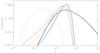Fig. 1 Distributions of the tSZ, φ, and CIB power as a function of the redshift at ℓ = 1000. The black solid line depicts the lensing potential, φ, the grey dashed line the tSZ effect, the dark blue, light blue, green, yellow, orange, and red dashed lines plot the CIB at 100, 143, 217, 353, 545, and 857 GHz, respectively.

2.3. Redshift distribution

In Fig. 1, we present the redshift distribution of power for the tSZ, CIB, and lensing potential auto-correlation spectra. The tSZ effect is produced by structures at low redshift (z< 2). The CIB and φ spectra are dominated by objects at higher redshift.

The mean redshift of structures that dominate in the CIB is a function of the considered frequency. These redshift windows highlight the high degree of correlation between the CIB and φ and the low degree of correlation between tSZ and the other two probes of large-scale structures.

For example, the high degree of correlation between the CIB and φ have recently been used to detect the lensing B modes of polarization by the SPT collaboration (Hanson et al., 2013).

Consequently, small CIB residuals in a tSZ Compton parameter map can lead to a significant bias in the tSZ-φ correlation analysis.

3. CIB-φ contamination in tSZ-φ cross-correlation

3.1. tSZ Compton parameter map

The recently released Planck data allow constructing full-sky tSZ Compton parameter map (Planck Collaboration XXI, 2014) using internal linear combination (ILC) component separation methods (see e.g., Remazeilles et al., 2011; Hurier et al., 2013). These methods reconstruct the tSZ signals using linear combinations $\mathit{y}\mathrm{=}\sum _{\mathit{\nu }}{\mathit{w}}_{\mathit{\nu }}{\mathit{T}}_{\mathit{\nu }}\mathit{,}$(14)where T_ν is the intensity at the frequency ν and w_ν are the weights of the linear combination. For ILC-based methods, these weights are computed by minimizing the variance of the reconstructed y-map under constraints.

The level of CIB-φ contamination in a tSZ-φ analysis based on a tSZ Compton parameter map depends on the weights, w_ν, used for the linear combination.

We here considered the weights provided in Table 2 of Hill & Spergel (2014), which have been used to constrain the cosmology from the tSZ-φ cross-correlation power-spectrum.

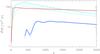Fig. 2 Residual contamination before cleaning in light blue and after cleaning in dark blue. The red solid line presents the tSZ-φ correlation for our fiducial model. The solid blue lines are the contamination considering the set of weights from Hill & Spergel (2014) for fsky = 0.3. The dashed blue lines are the contamination considering the set of weights from Hill & Spergel (2014) for fsky = 0.2.

3.2. Propagation of CIB-φ spectra

We stress that the CIB is composed of different populations of objects at different frequencies. The associated power-spectra present variations of shape with respect to the frequency. The CIB-φ spectra present the same variations of shape with frequency. The CIB-φ contamination in the tSZ-φ cross-correlation reads ${\mathit{C}}_{\mathit{\ell }}^{\mathrm{conta}}\mathrm{=}\sum _{\mathit{\nu }}{\mathit{w}}_{\mathit{\nu }}{\mathit{C}}_{\mathit{\ell }}^{\mathit{\phi }\mathrm{\times }\mathrm{CIB}\mathrm{\left(}\mathit{\nu }\mathrm{\right)}}\mathit{.}$(15)In Fig. 2, we present our estimation of the CIB-φ contamination considering the set of weights from Hill & Spergel (2014) and compare it with the expected tSZ-φ cross-correlation power-spectrum for our fiducial model.

The contamination is high, with a similar amplitude as the tSZ-φ correlation. Furthermore, the contamination level is highly dependent on the set of weights. For different sets of weights, the contamination varies an the same order of magnitude as the tSZ-φ signal.

This variability highlights the difficulty of controlling the CIB-φ contamination that can lead to a high bias in tSZ-φ analysis.

However, the contamination level is highly dependent on the exact CIB frequency correlation matrix. Consequently, the derived value has to be considered as an order-of-magnitude estimate of the effective contamination.

4. Cleaning the CIB-φ contamination

In their analysis, Hill & Spergel (2014) proposed a method of cleaning for CIB-φ contamination in tSZ-φ spectrum. Their method consists of a correction of the form ${\mathit{C}}_{\mathit{\ell }}^{\mathit{\phi }\mathrm{\times }\mathit{y,}\hspace{0.17em}\mathrm{corr}}\mathrm{=}{\mathit{C}}_{\mathit{\ell }}^{\mathit{\phi }\mathrm{\times }\mathit{y}}\mathrm{-}{\mathit{\alpha }}_{\mathrm{corr}}{\mathit{C}}_{\mathit{\ell }}^{\mathit{\phi }\mathrm{\times }\mathrm{CIB}\mathrm{\left(}\mathrm{857}\mathrm{\right)}}\mathit{,}$(16)where ${\mathit{C}}_{\mathit{\ell }}^{\mathit{\phi }\mathrm{\times }\mathit{y}}$ is the measured correlation between the tSZ and potential maps. The factor α_corr is computed from an adjustment of ${\mathit{C}}_{\mathit{\ell }}^{\mathrm{CIB}\mathrm{\left(}\mathrm{857}\mathrm{\right)}\mathrm{\times }\mathrm{CIB}\mathrm{\left(}\mathrm{857}\mathrm{\right)}}$ on the cross-correlation of the tSZ Compton parameter and the 857 GHz maps.

We propose to test the accuracy of this procedure using our modelling of the tSZ, φ, and CIB cross-correlations. In their analysis Hill & Spergel (2014) neglected the tSZ-CIB correlation contribution for computing α_corr. However, at the concerned frequencies, the tSZ-CIB correlation factor can reach about 20% and therefore cannot be neglected. Neglecting tSZ-CIB correlation for the cleaning process leads to an underestimation of the CIB-φ contamination. In an optimistic case³, α_corr reads 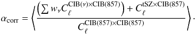${\mathit{\alpha }}_{\mathrm{corr}}\mathrm{=}⟨\frac{\mathrm{(}\sum {\mathit{w}}_{\mathit{\nu }}{{\mathit{C}}_{\mathit{\ell }}^{\mathrm{CIB}\mathrm{\left(}\mathit{\nu }\mathrm{\right)}\mathrm{\times }\mathrm{CIB}\mathrm{\left(}\mathrm{857}\mathrm{\right)}}}^{\mathrm{)}}\mathrm{+}{\mathit{C}}_{\mathit{\ell }}^{\mathrm{tSZ}\mathrm{\times }\mathrm{CIB}\mathrm{\left(}\mathrm{857}\mathrm{\right)}}}{{\mathit{C}}_{\mathit{\ell }}^{\mathrm{CIB}\mathrm{\left(}\mathrm{857}\mathrm{\right)}\mathrm{\times }\mathrm{CIB}\mathrm{\left(}\mathrm{857}\mathrm{\right)}}}⟩\mathrm{·}$(17)We computed this value for each set of weights at ℓ = 600. The value of α_corr varies by 3% depending on the value of ℓ used for the computation (300 <ℓ< 1500), with a higher level of contamination using higher ℓ values. Hill & Spergel (2014) found ${\mathit{\alpha }}_{\mathrm{corr}}\mathrm{=}\mathrm{(}\mathrm{6.7}\mathrm{\pm }\mathrm{1.1}\mathrm{)}\mathrm{\times }{\mathrm{10}}^{-6}\hspace{0.17em}{\mathrm{K}}_{\mathrm{CMB}}^{-1}$ for f_sky = 0.3. Considering the associated set of weight we predict ${\mathit{\alpha }}_{\mathrm{corr}}\mathrm{=}\mathrm{(}\mathrm{7.1}\mathrm{\pm }\mathrm{0.2}\mathrm{)}\mathrm{\times }{\mathrm{10}}^{-6}\hspace{0.17em}{\mathrm{K}}_{\mathrm{CMB}}^{-1}$ for 300 <ℓ< 1500. With this, we estimate the associated residual contamination in the tSZ-φ spectrum as 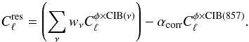${\mathit{C}}_{\mathit{\ell }}^{\mathrm{res}}\mathrm{=}\left(\sum _{\mathit{\nu }}{\mathit{w}}_{\mathit{\nu }}{\mathit{C}}_{\mathit{\ell }}^{\mathit{\phi }\mathrm{\times }\mathrm{CIB}\mathrm{\left(}\mathit{\nu }\mathrm{\right)}}\right)\mathrm{-}{\mathit{\alpha }}_{\mathrm{corr}}{\mathit{C}}_{\mathit{\ell }}^{\mathit{\phi }\mathrm{\times }\mathrm{CIB}\mathrm{\left(}\mathrm{857}\mathrm{\right)}}\mathit{.}$(18)In Fig. 2, we present the obtained residuals for the set of weights from Hill & Spergel (2014). The CIB-φ residual contributes with (20 ± 10)% of the tSZ-φ signal for ℓ ranging from 500 to 2000.

This level of contamination is dependent on the CIB luminosity function (see Sect. 2.2). The uncertainty level was estimated by propagating the CIB luminosity function uncertainties (see Planck Collaboration XXX, 2014, for details on estimating the CIB luminosity function parameters). This uncertainty level is dominated by δ_cib and ϵ_cib, which set the amount of correlation between the CIB maps observed at different frequencies. Other parameters, such as b_lin or CIB SED parameters, have a weaker effect on the CIB-φ residual estimation.

5. Conclusion and discussion

We have presented a modelling of the tSZ-φ-CIB cross-correlations. Based on this modelling, we predicted the expected CIB-φ contamination in the tSZ-φ power-spectra deduced from a Compton parameter map built by linearly combining Planck channels from 100 to 857 GHz.

We demonstrated that the expected level of contamination from the CIB-φ is at the same level as the tSZ-φ signal itself.

We also demonstrated that the CIB-φ contamination level is highly dependent on the set of weights used for constructing of the Compton parameter map. To do this, we used realistic values deduced from the sky, for the weights.

We tested a cleaning method for this bias and showed that the level of residual bias can reach about 20% of the tSZ-φ spectrum

for the used set of weights. Consequently, we stress that an tSZ-φ analysis that is based on a multi-frequency Compton parameter map may present a high level of bias. A careful CIB-φ analysis has to be performed simultaneously to a tSZ-φ analysis to avoid high bias in the final results.

Hill & Spergel (2014) constrained σ₈(Ω_m/ 0.282)^0.26 = 0.824 ± 0.029 and found that the tSZ-φ power-spectrum scales as ${\mathit{\sigma }}_{\mathrm{8}}^{\mathrm{6.1}}$. Thus, a bias of (20 ± 10)% on the the tSZ-φ amplitude produces a bias of (3.3 ± 1.7)% on the σ₈ amplitude. As a consequence, the CIB-φ induced residual bias in this measurement contributes about 1σ of the uncertainty. Such a bias may explain the difference between the tSZ-φ cross-correlation and cosmological parameter estimation made with a tSZ spectrum. The latter favours lower values for σ₈, with σ₈(Ω_m/ 0.28)^0.395 = 0.784 ± 0.016.

Acknowledgments

We are grateful to N. Aghanim and M. Douspis for useful discussions. We acknowledge the support of the French Agence Nationale de la Recherche under grant ANR-11-BD56-015.

References

All Tables

All Figures

	Fig. 1 Distributions of the tSZ, φ, and CIB power as a function of the redshift at ℓ = 1000. The black solid line depicts the lensing potential, φ, the grey dashed line the tSZ effect, the dark blue, light blue, green, yellow, orange, and red dashed lines plot the CIB at 100, 143, 217, 353, 545, and 857 GHz, respectively.
In the text

Fig. 2 Residual contamination before cleaning in light blue and after cleaning in dark blue. The red solid line presents the tSZ-φ correlation for our fiducial model. The solid blue lines are the contamination considering the set of weights from Hill & Spergel (2014) for fsky = 0.3. The dashed blue lines are the contamination considering the set of weights from Hill & Spergel (2014) for fsky = 0.2.

In the text

References

- Blanchard, A., & Schneider, J. 1987, A&A, 184, 1 [NASA ADS] [Google Scholar]
- Fixsen, D. J., Dwek, E., Mather, J. C., Bennett, C. L., & Shafer, R. A. 1998, ApJ, 508, 123 [NASA ADS] [CrossRef] [Google Scholar]
- Hanson, D., Hoover, S., Crites, A., et al. 2013, Phys. Rev. Lett., 111, 141301 [NASA ADS] [CrossRef] [PubMed] [Google Scholar]
- Hill, J. C., & Spergel, D. N. 2014, J. Cosmol. Astropart. Phys., 2, 30 [Google Scholar]
- Hurier, G., Macías-Pérez, J. F., & Hildebrandt, S. 2013, A&A, 558, A118 [NASA ADS] [CrossRef] [EDP Sciences] [Google Scholar]
- Komatsu, E., & Kitayama, T. 1999, ApJ, 526, L1 [NASA ADS] [CrossRef] [PubMed] [Google Scholar]
- Mo, H. J., & White, S. D. M. 1996, MNRAS, 282, 347 [NASA ADS] [CrossRef] [Google Scholar]
- Planck Collaboration XVII. 2014, A&A, 571, A17 [NASA ADS] [CrossRef] [EDP Sciences] [Google Scholar]
- Planck Collaboration XVIII. 2014, A&A, 571, A18 [NASA ADS] [CrossRef] [EDP Sciences] [Google Scholar]
- Planck Collaboration XX. 2014, A&A, 571, A20 [NASA ADS] [CrossRef] [EDP Sciences] [Google Scholar]
- Planck Collaboration XXI. 2014, A&A, 571, A21 [NASA ADS] [CrossRef] [EDP Sciences] [Google Scholar]
- Planck Collaboration XXX. 2014, A&A, 571, A30 [NASA ADS] [CrossRef] [EDP Sciences] [Google Scholar]
- Puget, J.-L., Abergel, A., Bernard, J.-P., et al. 1996, A&A, 308, L5 [NASA ADS] [Google Scholar]
- Remazeilles, M., Delabrouille, J., & Cardoso, J.-F. 2011, MNRAS, 410, 2481 [NASA ADS] [CrossRef] [Google Scholar]
- Shang, C., Haiman, Z., Knox, L., & Oh, S. P. 2012, MNRAS, 421, 2832 [NASA ADS] [CrossRef] [Google Scholar]
- Sunyaev, R. A., & Zeldovich, Y. B. 1969, Nature, 223, 721 [NASA ADS] [CrossRef] [Google Scholar]
- Sunyaev, R. A., & Zeldovich, Y. B. 1972, Comm. Astrophys. Space Phys., 4, 173 [Google Scholar]
- Tinker, J., Kravtsov, A. V., Klypin, A., et al. 2008, ApJ, 688, 709 [NASA ADS] [CrossRef] [Google Scholar]
All Tables
Cosmological and scaling-law parameters for our fiducial model for both Y500 − M500 (Planck Collaboration XX, 2014) and the L500 − M500 relation fitted on CIB spectra.