| Issue |
A&A
Volume 575, March 2015
|
|
|---|---|---|
| Article Number | L15 | |
| Number of page(s) | 10 | |
| Section | Letters | |
| DOI | https://doi.org/10.1051/0004-6361/201425570 | |
| Published online | 05 March 2015 | |
The GAPS programme with HARPS-N at TNG
VI. The curious case of TrES-4b⋆,⋆⋆
1 INAF–Osservatorio Astrofisico di Torino, via Osservatorio 20, 10025 Pino Torinese, Italy
e-mail: This email address is being protected from spambots. You need JavaScript enabled to view it.
2 INAF–Osservatorio Astrofisico di Catania, via S.Sofia 78, 95123 Catania, Italy
3 Max-Planck-Institut für Astronomie, Königstuhl 17, 69117 Heidelberg, Germany
4 INAF–Osservatorio Astronomico di Padova, Vicolo Osservatorio 5, 35122 Padova, Italy
5 INAF–Osservatorio Astronomico di Brera, via E. Bianchi 46, 23807 Merate (LC), Italy
6 INAF–Osservatorio Astronomico di Palermo, Piazza del Parlamento, Italy 1, 90134 Palermo, Italy
7 Landessternwarte Königstuhl, Zentrum für Astronomie der Universitat Heidelberg, Königstuhl 12, 69117 Heidelberg, Germany
8 INAF–Osservatorio Astronomico di Trieste, via Tiepolo 11, 34143 Trieste, Italy
9 Harvard-Smithsonian Center for Astrophysics, 60 Garden Street, Cambridge, Massachusetts, 02138, USA
10 Dipartimento di Fisica, Università di Milano, via Celoria 16, 20133 Milano, Italy
11 Dip. di Fisica e Astronomia Galileo Galilei–Università di Padova, Vicolo dell’Osservatorio 2, 35122 Padova, Italy
12 Fundación Galileo Galilei – INAF, Rambla José Ana Fernandez Pérez 7, 38712 Breña Baja, TF, Spain
13 INAF–IASF Milano, via Bassini 15, 20133 Milano, Italy
14 Département d’Astronomie de l’Université de Genève, 51 ch. des Maillettes – Observatoire de Sauverny, 1290 Versoix, Switzerland
15 Instituto de Astrofísica e Ciências do Espaço, Universidade do Porto, Rua das Estrelas, 4150-762 Porto, Portugal
16 Departamento de Física e Astronomia, Faculdade de Ciências, Universidade do Porto, Rua do Campo Alegre, 4169-007 Porto, Portugal
17 Lowell Observatory, 1400 W. Mars Hill Road, Flagstaff, AZ 86001, USA
18 Astrophysics Group, Keele University, Staffordshire, ST5 5BG, UK
Received: 22 December 2014
Accepted: 19 January 2015
Abstract
We update the TrES-4 system parameters using high-precision HARPS-N radial-velocity measurements and new photometric light curves. A combined spectroscopic and photometric analysis allows us to determine a spectroscopic orbit with a semi-amplitude K = 51 ± 3 m s-1. The derived mass of TrES-4b is found to be Mp = 0.49 ± 0.04 MJup, significantly lower than previously reported. Combined with the large radius (Rp = 1.84-0.09+0.08 RJup) inferred from our analysis, TrES-4b becomes the transiting hot Jupiter with the second-lowest density known. We discuss several scenarios to explain the puzzling discrepancy in the mass of TrES-4b in the context of the exotic class of highly inflated transiting giant planets.
Key words: stars: individual: TrES-4b / planetary systems / techniques: radial velocities / techniques: spectroscopic / techniques: photometric
Based on observations made with the Italian Telescopio Nazionale Galileo (TNG) operated on the island of La Palma by the Fundacion Galileo Galilei of the INAF at the Spanish Observatorio del Roque de los Muchachos of the IAC in the frame of the program Global Architecture of Planetary Systems (GAPS), and with the Zeiss 1.23-m telescope at the German-Spanish Astronomical Center at Calar Alto, Spain.
Tables 1 and 3 are available in electronic form at http://www.aanda.org
© ESO, 2015
1. Introduction
The class of transiting extrasolar planets (more than 1000 are either confirmed or validated to date) allows for many a study to further our understanding of their interiors, atmospheres, and ultimately, of their formation and evolution history (see, e.g., Madhusudhan et al. 2014 and Baraffe et al. 2014). The subset of close-in giant planetary companions (hot Jupiters) with very large radii and corresponding very low mean densities for a time posed a conundrum to theoreticians (the so-called radius anomaly problem; see, e.g., Bodenheimer et al. 2003). There is now growing consensus that the radius of a hot Jupiter can be inflated by several factors, including variable stellar irradiation, the planet mass and heavy element content, tidal and kinetic heating, and Ohmic dissipation (for a review see, e.g., Spiegel et al. 2014, and references therein).
The distribution of planetary radii of transiting hot Jupiters in systems with well-determined stellar and planetary parameters has been described in the recent past in terms of some of the relevant factors (such as equilibrium temperature, stellar metallicity, and orbital semi-major axis) using empirical formulae based on the assumption of independent variables (Béky et al. 2011; Enoch et al. 2011) or a multivariate regression approach (Enoch et al. 2012; Weiss et al. 2013). These latest models are quite successful in statistically reproducing the observed radius distribution of this class of exoplanets. Still, some of the most extreme planets with the largest radii remain challenging for current models of planetary formation and bulk structure. For example, the extremely low densities of objects such as WASP-17b (Anderson et al. 2010), HAT-P-32b (Hartman et al. 2011), WASP-79b (Smalley et al. 2012), WASP-88b (Delrez et al. 2014), or Kepler-12b (Fortney et al. 2011) cannot be reproduced by simple models of core-less planets (e.g., Baraffe et al. 2014), nor can the atmospheric inflation mechanisms mentioned above explain the observed radii.
TrES-4b (Mandushev et al. 2007, M07 thereafter) is another highly bloated transiting hot Jupiter. It belongs to the restricted group of some dozen objects with a measured radius larger than 1.7 RJup (Sozzetti et al. 2009, S09 thereafter; Chan et al. 2011; Sada et al. 2012; Southworth et al. 2012). Measurements of the Rossiter-McLaughlin effect (Narita et al. 2010, N10 hereafter) revealed close spin-orbit alignment of the TrES-4 system. Atmospheric characterization measurements have been obtained by Knutson et al. (2009), who detected a temperature inversion in the TrES-4b broadband infrared emission spectrum with Spitzer/IRAC during secondary eclipse, and by Ranjan et al. (2014), who presented a featureless transmission spectrum of TrES-4b using HST/WFC3 during primary transit. Constraints from the secondary eclipse measurements and expanded radial-velocity (RV) datasets (Knutson et al. 2014, K14 thereafter) indicate a probable circular orbit for TrES-4b. Using a time baseline in excess of five years, K14 did not detect any significant acceleration in the RV data that would indicate that the system has a massive outer companion. Finally, TrES-4 has a faint common proper motion companion at ~ 1.5′′ that was discovered by Daemgen et al. (2009) and confirmed by Bergfors et al. (2013).
In this Letter we present RV measurements of TrES-4 gathered with the HARPS-N spectrograph (Cosentino et al. 2012) at the Telescopio Nazionale Galileo (TNG) within the context of the programme Global Architecture of Planetary Systems (GAPS, Covino et al. 2013; Desidera et al. 2013), along with additional photometric light-curves during transit obtained with the Zeiss 1.23 m telescope at the German-Spanish Calar Alto Observatory (CAHA). A combined analysis allows us to derive a much lower mass for TrES-4b than previously reported, making it the transiting hot Jupiter with the second-lowest density known to-date.
2. Spectroscopic and photometric observations
The TrES-4 system was observed with HARPS-N on 17 individual epochs between March 2013 and July 2014. The Th-Ar simultaneous calibration was not used to avoid contaminating the stellar spectrum by the lamp lines (which would affect a proper spectral analysis). In addition, the magnitude of the instrumental drift during a night (≲ 1 m s-1) is considerably lower than the typical photon-noise RV errors (≃ 9 m s-1), thus of no impact for faint stars such as TrES-4 (see, e.g., Bonomo et al. 2014; Damasso et al. 2015). We reduced the spectra and RV measurements with the latest version (Nov. 2013) of the HARPS-N instrument data reduction software (DRS) pipeline and the G2 mask. We measured the RVs using the weighted cross-correlation function (CCF) method (Baranne et al. 1996; Pepe et al. 2002). The individual measurements are reported in Table 1, together with the values of the bisector span and the chromospheric activity index  .
.
The spectra of TrES-4 were coadded to produce a merged spectrum with a peak signal-to-noise ratio of ~ 110 pixel-1 at 550 nm. We determined the atmospheric stellar parameters using the code MOOG (Sneden 1973; version 2013) and implemented both methods based on equivalent widths and on spectral synthesis, as described in Biazzo et al. (2012), D’Orazi et al (2011), and Gandolfi et al. 2013. The final adopted parameters are listed in Table 2.
System parameters of TrES-4.
We carried out Ic-band precision photometric observations of two complete transit events of TrES-4 b with the CAHA 1.23-m on UT 2013 July 6 and UT 2014 June 30. The telescope was defocussed and autoguided during all the observations, and the CCD was windowed to reduce the readout time. The datasets were reduced using standard calibration techniques (overscan correction, trimming, bias subtraction, flat fielding). We then derived differential fluxes relative to an ensemble of local comparison stars (using the methodology described in Southworth et al. 2014). The final set of photometric time series of TrES-4 is available in Table 3. Uncertainties on individual photometric measurements were estimated separately for the two light curves as the standard deviation of the transit-fitting residuals; these uncertainties are larger than the formal error bars in both cases. Correlated noise was then estimated following Pont et al. (2006) and Bonomo et al. (2012) and added in quadrature with the individual measurement uncertainties. Final uncertainties are equal to 8.42 × 10⁻⁴ and 7.71 × 10⁻⁴ (in units of relative flux) for the former and latter light curve, respectively.
3. Revised TrES-4 system parameters
New parameters of the TrES-4 system were derived through a Bayesian combined analysis of our photometry in Ic band and HARPS-N RV measurements by simultaneously fitting a transit model (Giménez, 2006, 2009) and a Keplerian orbit. For this purpose, we used a differential evolution Markov chain Monte Carlo method (Ter Braak 2006; Eastman et al. 2013) with a Gaussian likelihood function (see, e.g., Gregory 2005). Our global model has eleven free parameters: the transit epoch T0; the orbital period P; the systemic radial velocity γ; the radial-velocity semi-amplitude K; e cosω and e sinω, where e is the eccentricity and ω the argument of periastron; an error term added in quadrature to the formal uncertainties to account for possible jitter in the RV measurements regardless of its origin, such as instrumental effects and stellar activity; the transit duration from first to fourth contact T14; the ratio of the planet to stellar radii Rp/R∗; the inclination i between the orbital plane and the plane of the sky; and the coefficient u of a linear limb-darkening law. We first tried to use a quadratic limb-darkening law, but the two coefficients, especially the quadratic one, were highly unconstrained. This means that the precision of our transit light curves does not allow fitting both coefficients.
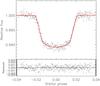 |
Fig. 1 Phase-folded observations of two full transits of TrES-4b in Ic band along with the best-fit model (red solid line). See Sect. 3 for details. |
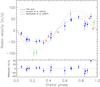 |
Fig. 2 Top panel: phase-folded RV measurements of TrES-4 obtained with HARPS-N (blue circles) and, superimposed, the best-fit Keplerian orbit model (black solid line). The Keck/HIRES RVs from M07 (green diamonds) and K14 (red squares) and the two best-fit orbital solutions obtained in these papers are also shown. Bottom panel: residuals from the best-fit model to the HARPS-N RVs. |
Gaussian priors were imposed on T0 and P after improving the transit ephemeris by combining the transit epochs available in the literature (M07; Chan et al. 2011) with the two epochs we derived from our Ic photometry by analyzing each individual transit with a circular transit model and a DE-MCMC technique. Gaussian priors were also set on the center times of the secondary eclipses observed by Knutson et al. (2009) with the Spitzer Space Telescope because they provide strong constraints on e cosω (e.g., Jordán & Bakos 2008). Non-informative priors were used for the other orbital and transit parameters, while a modified Jeffrey’s prior was adopted for the RV jitter term.
The DE-MCMC analysis was stopped after it reached convergence and good mixing of the chains (Ford, 2006). The final best-fit transit model and RV curve are overplotted on the phase-folded data in Figs. 1 and 2, respectively. We did not determine a significant RV jitter, listed as an upper limit in Table 2 (only internal errors are reported in Table 1 and Fig. 2). The density of the host star from the transit fitting and the effective temperature and stellar metallicity as derived in Sect. 2 were later compared with the theoretical Yonsei-Yale evolutionary tracks (Demarque et al., 2004) to determine the stellar mass, radius, surface gravity, age, and their associated uncertainties (Sozzetti et al., 2007; Torres et al., 2012). They are listed in Table 2 and agree within 1σ with the literature values (cf., e.g., Torres et al. 2008; Chan et al. 2011). The related planetary parameters are Mp = 0.494 ± 0.035 MJup, 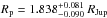 , and
, and 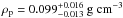 .
.
4. Discussion and conclusions
Our new, combined spectroscopic and photometric analysis of the TrES-4 system allows us to determine stellar properties in good agreement (within the errors) with the properties measured by M07 and S09. The planetary radius also agrees well with the most recent determinations by S09 and Chan et al. (2011), although we formally derive its highest value to date. One striking element emerges from our study, however. The best-fit Keplerian orbit for TrES-4 based on HARPS-N RV measurements (K = 51 ± 3 m s-1) has an amplitude almost a factor 2 smaller than that (K = 97 ± 7 m s-1) reported by M07. As a consequence, the revised mass of the planet is ~ 1.7 times lower. This discrepancy clearly deserves a thorough investigation, and we describe here the steps we have taken in this direction.
In the most recent update of the TrES-4 system parameters, K14 reported K = 84 ± 10 m s-1 and  MJup. These numbers are compatible within the error bars with the initial estimates of M07 and S09. The orbital solution of K14 is based on the combination of three datasets, from M07, N10, and obtained by the authors themselves. We show in Fig. 2 a phase plot of the published Keck velocities and our HARPS-N dataset, superposed on the three orbital solutions derived by M07, K14, and in this work (the N10 RV set obtained with Subaru/HDS is of significantly lower internal precision and is not shown). The RVs published by M07 are clearly incompatible with the K-value derived based on HARPS-N RV data. The data obtained by K14 did not sample the critical orbital phases, and they appear consistent with both solutions. The higher K-value in the Keck data is thus driven by the observations of the discovery paper.
There are several scenarios that can be proposed to explain the observed discrepancy in the RV amplitudes. One possible culprit might be the faint companion at ~ 1.5′′ (almost due north of TrES-4). Cunha et al. (2013) have analyzed in detail the impact of faint stellar companions on precision RVs from spectra gathered with fiber-fed spectrographs. The companion of TrES-4 is of late-K or early-M spectral type and ≈ 4.5 mag fainter at i-band. From Table 8 of Cunha et al. (2013) one then infers that contamination levels between 1 and 10 m s-1 could apply if the companion were to fall within the fiber of HARPS-N. A systematic effect of similar magnitude might be induced on the Keck RVs if the companion had been on the HIRES slit during the period of the M07 observations. Either way, this scenario does not seem to provide a convincing explanation for the observed difference in the K-value, as the higher RV dispersion inferred does not have the required magnitude and, most importantly, this effect would have had to occur in such a way as to exactly double (or halve) the signal amplitude. The hypothesis of large starspots on the stellar photosphere (causing an apparent RV shift on a timescale of the stellar rotation period) is unlikely for a late F-star such as TrES-4 (see Knutson et al. 2009). Large, intrinsic stellar jitter also does not appear to be supported by the observational evidence. No emission is seen in the Ca ii H and K lines related to magnetic activity in the HARPS-N spectra, from which we derive 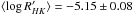 , essentially indistinguishable from the value reported by S09. The empirical relation by Wright (2005) predicts a typical stellar jitter of ~ 4 m s-1 for such a star as TrES-4. We note, however, that the very low value of the chromospheric emission is in line with the correlation found by Hartman (2010) and could be explained as the effect of absorption in the Ca ii H and K line cores by material evaporated from the low-gravity planet (Lanza 2014; Figueira et al. 2014). Based on the absence of bump progression in the mean line profiles of HARPS-N and archival Keck data (determined with the Donati et al. 1997 technique), we also rule out the possibility that the amplitude of the RV curve of TrES-4 is modified by nonradial stellar pulsations typical of γ Dor variables (Kaye et al. 1999), which have been detected in a few cases in stars with stellar parameters similar to those of TrES-4 (Uytterhoeven et al. 2014). A homogeneous, comprehensive re-analysis of all available Keck data on the system might help to resolve the conundrum, particularly to understand if unrecognized systematics in the few Keck RVs in the discovery paper might be to blame.
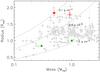 |
Fig. 3 Mass-radius diagram of the known transiting planets with Rp ≥ 0.4 RJup and Mp ≥ 0.1 MJup. Only systems with masses determined to better than 30% precision are included. Green diamonds indicate the solar system giant planets Jupiter and Saturn (from right to left). The three dotted lines display isodensity curves of 0.1, 0.5, and 1.5 g cm-3. The position of TrES-4b as determined in this work is shown with a filled red square, to be compared with that (empty red square) derived by S09. |
The much lower mass of TrES-4b as determined by HARPS-N implies a significantly lower density than previously thought for this hot Jupiter. The new location of TrES-4b in the mass-radius diagram of known transiting giant planets (Fig. 3) makes it the object with the second-lowest density, WASP-17b (Southworth et al. 2012; Bento et al. 2013) being the record-holder at present. With a mass closer to that of Saturn, the predicted radius of TrES-4b is significantly underestimated by all empirical relations recently proposed in the literature (Béky et al. 2011; Enoch et al. 2011, 2012; Weiss et al. 2013), with radius differences ranging between 0.74 RJup and 0.45 RJup. In a Rp − Teq diagram (see Fig. 4 for details), TrES-4b nicely fits in the upper envelope of lowest-density objects, which exhibit a strong positive correlation between the two parameters (Spearman rank correlation coefficient rs = 0.82 ± 0.03). We note how the trend of increasing Rp with Teq becomes significantly milder if we consider the sample of the densest giants (rs = 0.54 ± 0.06), and for these the relationship becomes completely flat if a cutoff of about 1.0 RJup is adopted (instead of the one used in Fig. 4).
We confirm a very low eccentricity (e< 0.016 at the 1σ level) for the orbit of TrES-4b, improving upon the recent determination by K14. An estimate of the typical tidal timescales based on the model by Leconte et al. (2010) adapted so as to allow constant modified tidal quality factors for the star ( ) and the planet (
 ) gives a circularization timescale of 40 Myr, which supports the e ≃ 0 hypothesis. On the other hand, the evolution timescale of the obliquity obtained with the same tidal model is ~ 24 Gyr, while that for the orbital decay is ~ 6 Gyr. This suggests that the alignment of the system is primordial and that no remarkable tidal evolution of the orbit has occurred during the main-sequence lifetime of the system. With the currently derived upper limit for the eccentricity, the maximum power dissipated by equilibrium tides inside the planet is ~ 4.5 × 10¹⁸ W, which is not enough to explain its large radius anomaly. Given its peculiarity, further photometric and spectroscopic monitoring of the TrES-4 planetary system is clearly encouraged.
 |
Fig. 4 Dependence on equilibrium temperature of the observed radii of giant planets with Mp ≥ 0.1 MJup and Rp ≥ 0.8 RJup (data from http://exoplanet.eu/). Purple squares, gray circles, and green triangles indicate objects with ρp ≤ 0.25 g cm-3, 0.25 <ρp< 1.5 g cm-3, and ρp ≥ 1.5 g cm-3, respectively. The location of TrES-4b is shown with a red square. |
Online material
HARPS-N radial velocities, formal errors, bisector spans, and chromospheric activity index of TrES-4.
Differential photometry of TrES-4.
Acknowledgments
The GAPS project in Italy acknowledges support from INAF through the “Progetti Premiali” funding scheme of the Italian Ministry of Education, University, and Research. We thank the TNG staff for help with the observations. This research has made use of the results produced by the PI2S2 Project managed by the Consorzio COMETA, a co-funded project by the Italian Ministero dell’Istruzione, Università e Ricerca (MIUR) within the Piano Operativo Nazionale Ricerca Scientifica, Sviluppo Tecnologico, Alta Formazione (PON 2000-2006). N.C.S. acknowledges the support from the ERC/EC under the FP7 through Starting Grant agreement n. 239953, from Fundação para a Ciência e a Tecnologia (FCT, Portugal), and POPH/FSE (EC) through FEDER funds in program COMPETE, as well as through and national funds, in the form of grants references RECI/FIS-AST/0176/2012 (FCOMP-01-0124-FEDER-027493), RECI/FIS-AST/0163/2012 (FCOMP-01-0124-FEDER-027492), and IF/00169/2012. Operations at the Calar Alto telescope are jointly performed by the Max-Planck Institut für Astronomie (MPIA) and the Instituto de Astrofísica de Andalucía (CSIC).
References
- Anderson, D. R., Hellier, C., Gillon, M., et al. 2010, ApJ, 709, 159 [NASA ADS] [CrossRef] [Google Scholar]
- Anderson, D. R., Smith, A. M. S., Lanotte, A. A., et al. 2011, MNRAS, 416, 2108 [NASA ADS] [CrossRef] [Google Scholar]
- Baraffe, I., Chabrier, G., Fortney, J., & Sotin, C. 2014, in Protostars and Planets VI (University of Arizona Press), eds. H. Beuther, R. Klessen, C. Dullemond, & Th. Henning, 763 [Google Scholar]
- Baranne, A., Queloz, D., Mayor, M., et al. 1996, A&AS, 119, 373 [NASA ADS] [CrossRef] [EDP Sciences] [Google Scholar]
- Béky, B., Bakos, G. A., Hartman, J., et al. 2011, ApJ, 734, 109 [NASA ADS] [CrossRef] [Google Scholar]
- Bento, J., Wheatley, P. J., Copperwheat, C. M., et al. 2013, MNRAS, 437, 1511 [NASA ADS] [CrossRef] [Google Scholar]
- Bergfors, C., Brandner, W., Daemgen, S., et al. 2013, MNRAS, 428, 182 [NASA ADS] [CrossRef] [Google Scholar]
- Biazzo, K., D’Orazi, V., Desidera, S., et al. 2012, MNRAS, 427, 2905 [NASA ADS] [CrossRef] [Google Scholar]
- Bodenheimer, P., Laughlin, G., & Lin, D. N. C. 2003, ApJ, 592, 555 [NASA ADS] [CrossRef] [Google Scholar]
- Bonomo, A. S., Chabaud, P. Y., Deleuil, M., et al. 2012, A&A, 547, A110 [NASA ADS] [CrossRef] [EDP Sciences] [Google Scholar]
- Bonomo, A. S., Sozzetti, A., Lovis, C., et al. 2014, A&A, 572, A2 [NASA ADS] [CrossRef] [EDP Sciences] [Google Scholar]
- Chan, T., Ingemyr, M., Winn, J. N., et al. 2011, AJ, 141, 179 [NASA ADS] [CrossRef] [Google Scholar]
- Cosentino, R., Lovis, C., Pepe, F., et al. 2012, Proc. SPIE, 8446, 84461V [Google Scholar]
- Covino, E., Esposito, M., Barbieri, M., et al. 2013, A&A, 554, A28 [NASA ADS] [CrossRef] [EDP Sciences] [Google Scholar]
- Cunha, D., Figueira, P., Santos, N. C., et al. 2013, A&A, 550, A75 [NASA ADS] [CrossRef] [EDP Sciences] [Google Scholar]
- Daemgen, S., Hormuth, F., Brandner, W., et al. 2009, A&A, 498, 567 [NASA ADS] [CrossRef] [EDP Sciences] [Google Scholar]
- Damasso, M., Biazzo, K., Bonomo, A. S., et al. 2015, A&A, 575, A111 [NASA ADS] [CrossRef] [EDP Sciences] [Google Scholar]
- Delrez, L., Van Grootel, V., Anderson, D. R., et al. 2014, A&A, 563, A143 [NASA ADS] [CrossRef] [EDP Sciences] [Google Scholar]
- Demarque, P., Woo, J.-H., Kim, Y.-Ch., & Yi, S. K. 2004, ApJS, 155, 667 [NASA ADS] [CrossRef] [Google Scholar]
- Desidera, S., Sozzetti, A., Bonomo, A. S., et al. 2013, A&A, 554, A29 [NASA ADS] [CrossRef] [EDP Sciences] [Google Scholar]
- Donati, J. F., Semel, M., Carter, B. D., Rees, D. E., & Collier Cameron, A. 1997, MNRAS, 291, 658 [NASA ADS] [CrossRef] [MathSciNet] [Google Scholar]
- D’Orazi, V., Biazzo, K., Randich, S. 2011, A&A, 526, A103 [NASA ADS] [CrossRef] [EDP Sciences] [Google Scholar]
- Eastman, J., Gaudi, B. S., & Agol, E. 2013, PASP, 125, 923 [Google Scholar]
- Enoch, B., Collier Cameron, A., Anderson, D. R., et al. 2011, MNRAS, 410, 1631 [NASA ADS] [Google Scholar]
- Enoch, B., Collier Cameron, A., & Horne, K. 2012, A&A, 540, A99 [NASA ADS] [CrossRef] [EDP Sciences] [Google Scholar]
- Figueira, P., Oshagh, M., Adibekyan, V. Zh., & Santos, N. C. 2014, A&A, 572, A51 [NASA ADS] [CrossRef] [EDP Sciences] [Google Scholar]
- Ford, E. B. 2006, ApJ, 642, 505 [NASA ADS] [CrossRef] [Google Scholar]
- Fortney, J. J., Demory, B.-O., Désert, J.-M., et al. 2011, ApJS, 197, 9 [NASA ADS] [CrossRef] [Google Scholar]
- Gandolfi, D., Parviainen, H., Fridlund, M., et al. 2013, A&A, 557, A74 [NASA ADS] [CrossRef] [EDP Sciences] [Google Scholar]
- Giménez, A. 2006, A&A, 450, 1231 [NASA ADS] [CrossRef] [EDP Sciences] [Google Scholar]
- Giménez, A. 2009, ASPC, 404, 291 [NASA ADS] [Google Scholar]
- Gregory, P. C. 2005, ApJ, 631, 1198 [NASA ADS] [CrossRef] [Google Scholar]
- Hartman, J. D. 2010, ApJ, 717, L138 [NASA ADS] [CrossRef] [Google Scholar]
- Hartman, J. D., Bakos, G. Á., Torres, G., et al. 2011, ApJ, 742, 59 [NASA ADS] [CrossRef] [Google Scholar]
- Jordán, A., & Bakos, G. Á. 2008, ApJ, 685, 543 [NASA ADS] [CrossRef] [Google Scholar]
- Kaye, A., Handler, G., Krisciunas, K., Poretti, E., & Zerbi, F.M. 1999, PASP, 111, 840 [NASA ADS] [CrossRef] [Google Scholar]
- Knutson, H. A., Charbonneau, D., Burrows, A., O’Donovan, F. T., & Mandushev, G. 2009, ApJ, 691, 866 [NASA ADS] [CrossRef] [Google Scholar]
- Knutson, H. A., Fulton, B. J., Montet, B. T., et al. 2014, ApJ, 785, 126 [NASA ADS] [CrossRef] [Google Scholar]
- Lanza, A.F. 2014, A&A, 572, L6 [NASA ADS] [CrossRef] [EDP Sciences] [Google Scholar]
- Leconte, J., Chabrier, G., Baraffe, I., & Levrard, B. 2010, A&A, 516, A64 [NASA ADS] [CrossRef] [EDP Sciences] [Google Scholar]
- Madhusudhan, N., Knutson, H., Fortney, J., & Barman, T. 2014, in Protostars and Planets VI (University of Arizona Press), eds. H. Beuther, R. Klessen, C. Dullemond, & Th. Henning, 739 [Google Scholar]
- Mandushev, G., O’Donovan, F. T., Charbonneau, D., et al. 2007, ApJ, 667, L195 [NASA ADS] [CrossRef] [Google Scholar]
- Narita, N., Sato, B., Hirano, T., et al. 2010, PASJ, 62, 653 [NASA ADS] [Google Scholar]
- Pepe, F., Mayor, M., Galland, F., et al. 2002, A&A, 388, 632 [NASA ADS] [CrossRef] [EDP Sciences] [Google Scholar]
- Pont, F., Zucker, S., & Queloz, D. 2006, MNRAS, 373, 231 [NASA ADS] [CrossRef] [Google Scholar]
- Ranjan, S., Charbonneau, D., Désert, J.-M., et al. 2014, ApJ, 785, 148 [NASA ADS] [CrossRef] [Google Scholar]
- Sada, P. V., Deming, D., Jennings, D. E., et al. 2012, PASP, 124, 212 [NASA ADS] [CrossRef] [Google Scholar]
- Smalley, B., Anderson, D. R., Collier Cameron, A., et al. 2012, A&A, 547, A61 [NASA ADS] [CrossRef] [EDP Sciences] [Google Scholar]
- Sneden, C. A. 1973, ApJ, 184, 839 [NASA ADS] [CrossRef] [Google Scholar]
- Southworth, J. 2012, MNRAS, 426, 1291 [NASA ADS] [CrossRef] [Google Scholar]
- Southworth, J., Hinse, T. C., Dominik, M., et al. 2012, MNRAS, 426, 1338 [NASA ADS] [CrossRef] [Google Scholar]
- Southworth, J., Hinse, T. C., Burgdorf, M., et al. 2014, MNRAS, 444, 776 [NASA ADS] [CrossRef] [Google Scholar]
- Sozzetti, A., Torres, G., Charbonneau, D., et al. 2007, ApJ, 664, 1190 [NASA ADS] [CrossRef] [Google Scholar]
- Sozzetti, A., Torres, G., Latham, D. W., et al. 2009, ApJ, 691, 1145 [NASA ADS] [CrossRef] [Google Scholar]
- Spiegel, D. S., Fortney, J. J., & Sotin, C. 2014, PNAS, 111, 12622 [NASA ADS] [CrossRef] [Google Scholar]
- Ter Braak, C. J. F. 2006, Statistics and Computing, 16, 239 [Google Scholar]
- Torres, G., Winn, J. N., & Holman, M. J. 2008, ApJ, 677, 1324 [NASA ADS] [CrossRef] [Google Scholar]
- Torres, G., Fischer, D. A., Sozzetti, A., et al. 2012, ApJ, 757, 161 [NASA ADS] [CrossRef] [Google Scholar]
- Uytterhoeven, K., Moya, A., Grigahcène, A., et al. 2011, A&A, 534, A125 [NASA ADS] [CrossRef] [EDP Sciences] [Google Scholar]
- Weiss, L. M., Marcy, G. W., Rowe, J. F., et al. 2013, ApJ, 768, 14 [NASA ADS] [CrossRef] [Google Scholar]
- Wright, J. T. 2005, PASP, 117, 657 [NASA ADS] [CrossRef] [Google Scholar]
All Tables
HARPS-N radial velocities, formal errors, bisector spans, and chromospheric activity index of TrES-4.
All Figures
|
Fig. 1 Phase-folded observations of two full transits of TrES-4b in Ic band along with the best-fit model (red solid line). See Sect. 3 for details. |
| In the text | |
|
Fig. 2 Top panel: phase-folded RV measurements of TrES-4 obtained with HARPS-N (blue circles) and, superimposed, the best-fit Keplerian orbit model (black solid line). The Keck/HIRES RVs from M07 (green diamonds) and K14 (red squares) and the two best-fit orbital solutions obtained in these papers are also shown. Bottom panel: residuals from the best-fit model to the HARPS-N RVs. |
| In the text | |
|
Fig. 3 Mass-radius diagram of the known transiting planets with Rp ≥ 0.4 RJup and Mp ≥ 0.1 MJup. Only systems with masses determined to better than 30% precision are included. Green diamonds indicate the solar system giant planets Jupiter and Saturn (from right to left). The three dotted lines display isodensity curves of 0.1, 0.5, and 1.5 g cm-3. The position of TrES-4b as determined in this work is shown with a filled red square, to be compared with that (empty red square) derived by S09. |
| In the text | |
|
Fig. 4 Dependence on equilibrium temperature of the observed radii of giant planets with Mp ≥ 0.1 MJup and Rp ≥ 0.8 RJup (data from http://exoplanet.eu/). Purple squares, gray circles, and green triangles indicate objects with ρp ≤ 0.25 g cm-3, 0.25 <ρp< 1.5 g cm-3, and ρp ≥ 1.5 g cm-3, respectively. The location of TrES-4b is shown with a red square. |
| In the text | |
Current usage metrics show cumulative count of Article Views (full-text article views including HTML views, PDF and ePub downloads, according to the available data) and Abstracts Views on Vision4Press platform.
Data correspond to usage on the plateform after 2015. The current usage metrics is available 48-96 hours after online publication and is updated daily on week days.
Initial download of the metrics may take a while.