| Issue |
A&A
Volume 575, March 2015
|
|
|---|---|---|
| Article Number | A113 | |
| Number of page(s) | 11 | |
| Section | Cosmology (including clusters of galaxies) | |
| DOI | https://doi.org/10.1051/0004-6361/201425016 | |
| Published online | 06 March 2015 | |
On the origin of intrinsic alignment in cosmic shear measurements: an analytic argument⋆
1 University of Milan, Department of Physics, via Celoria 16, 20133 Milan, Italy
e-mail: giovanni.camelio@roma1.infn.it
2 University of Rome “Sapienza”, Department of Physics, p.le Aldo Moro 2, 00185 Rome, Italy
3 Harvard-Smithsonian Center for Astrophysics, 60 Garden Street, Cambridge, MA 02138, USA
Received: 17 September 2014
Accepted: 31 December 2014
Galaxy intrinsic alignment can be a severe source of error in weak-lensing studies. The problem has been widely studied by numerical simulations and with heuristic models, but without a clear theoretical justification of its origin and amplitude. In particular, it is still unclear whether intrinsic alignment of galaxies is dominated by formation and accretion processes or by the effects of the instantaneous tidal field acting upon them. We investigate this question by developing a simple model of intrinsic alignment for elliptical galaxies, based on the instantaneous tidal field. Making use of the galaxy stellar distribution function, we estimate the intrinsic alignment signal and find that although it has the expected dependence on the tidal field, it is too weak to account for the observed signal. This is an indirect validation of the standard view that intrinsic alignment is caused by formation and/or accretion processes.
Key words: gravitational lensing: weak / galaxies: kinematics and dynamics / galaxies: halos
Appendices are available in electronic form at http://www.aanda.org
© ESO, 2015
1. Introduction
It has long been recognized that gravitational lensing is a particularly robust method to investigate the mass distribution of massive astronomical objects (e.g., see Refsdal 1964; Fu et al. 2008; Jauzac et al. 2012). Gravitational lensing is insensitive to the chemical and physical state of the deflecting matter and therefore treats ordinary and dark matter components of the deflector equally. In addition, it depends on a clearly understood physical process, the distortion of the space-time induced by masses as described by General Relativity, for which it is not required that the deflector be in a state of dynamical equilibrium. As a result, it currently represents our best tool to study the matter distribution in the Universe.
A particularly important use of weak-lensing methods, which are based on the statistical analysis of the weak correlation among the observed shapes of distant galaxies, is studying the large-scale structure of the Universe. In weak cosmological lensing, the deflecting matter studied (in contrast to the case of a cluster of galaxies) is distributed along the entire line of sight. As a result, the distinction between source and lens is less clear: the light of every galaxy that contributes to the distortion of space-time is bent by the distribution of matter along its path. The correlation between the apparent ellipticities of every pair of galaxies determines the signal; this is called cosmic shear. Since cosmic shear is related to the power spectrum of the density contrast (e.g., see Miralda-Escudé 1991; Kaiser 1992), with this tool one measures the statistical properties of the large-scale structure in the Universe. Therefore, weak cosmological lensing is an independent method for testing cosmological models (e.g., see Kilbinger et al. 2013).
Cosmic-shear measurements are particularly challenging: the signal is very weak and is affected by many error sources. From the modeling point of view, one of the main difficulties is related to the so-called intrinsic alignment, that is, the galaxy intrinsic shape alignment, which is not caused by gravitational lensing, but by the source gravitational field (Heavens et al. 2000; Croft & Metzler 2000; see also Troxel & Ishak 2014, for a recent review). Although the effects of intrinsic alignment can be reduced by removing pairs of galaxies that are physically close to the measurement of the shear correlation (King & Schneider 2002; Heymans & Heavens 2003), there remains a residual bias (called GI mode, see below). Therefore, it is important to clarify these effects and to assess their impact on current and future cosmic-shear surveys. Although some heuristic models for intrinsic alignment are available (e.g., Catelan et al. 2001; Hirata & Seljak 2004), they are unfortunately incomplete; in particular, they lack an analytic estimate of the bias magnitude (in general, such an estimate would require the use of complicated galaxy formation and stellar dynamical models). Therefore, one has to resort to the bias magnitude measured from simulations (Croft & Metzler 2000; Heavens et al. 2000; Jing 2002; Heymans et al. 2006; Tenneti et al. 2014) for a comparison with the observations.
The exact origin of intrinsic alignment is still debated (e.g., see Pereira & Kuhn 2005), and it is still unclear whether intrinsic alignment of galaxies is dominated by formation and accretion processes or by the effects of the instantaneous tidal field acting upon them. The commonly accepted view, supported by simulations and observations, is that the intrinsic alignment is caused by the tidal field acting at the formation epoch (Catelan et al. 2001; Hirata & Seljak 2004) and possibly on the merger history. In this paper we strengthen this view with analytic arguments using a reductio ad absurdum: that is, we start with the assumption that intrinsic alignment is dominated by the instantaneous tidal field currently at work on galaxies and show that the predicted effect is several orders of magnitude weaker than the observed effect. In our model, we consider a spherical early-type galaxy and study the deformation of its shape to first order after introducing a weak external tidal field. We describe the effects of the external tidal field on the intrinsic (i.e., unlensed) shape of the elliptical galaxy, determining the luminous quadrupole of the galaxy by means of its collisionless stellar distribution function. The galaxy ellipticity is then computed through the luminous quadrupole. We find the expected dependence of the ellipticity to the tidal field, as postulated by the heuristic model of Catelan et al. (2001), but the constant of proportionality determined by our model is more than four orders of magnitude lower than that observed (Joachimi et al. 2011), and consequently cannot account for the intrinsic alignment.
The paper is organized as follows: in Sect. 2 we present the problem of intrinsic alignment, summarize the relevant classifications, and outline the properties of different types of alignment. In Sect. 3 we introduce the stellar distribution function and estimate the ellipticity induced by an external tidal field on an elliptical galaxy. In Sect. 4 we compare our result with that of Joachimi et al. (2011) and apply our model to the galaxy dark matter halo. We draw our conclusions in Sect. 5. In Appendix A we study the dynamics of elliptical and spiral galaxies in the rigid-body approximation. Finally, in Appendix B, we derive an alternative intrinsic alignment ellipticity determined by instantaneous tidal fields by means of the equipotential surfaces of elliptical galaxies. Throughout this paper we take a standard cosmological model with Hubble constant H0 = 70 km s-1 kpc-1, mass density parameter Ωm = 0.3.
2. General context
2.1. Cosmic shear
In principle, unbiased shear measurements can be obtained from the luminous quadrupole tensor Qij of each galaxy in a given field of view (e.g., Bartelmann & Schneider 2001)  (1)where I(θ) is the surface brightness observed at angular position θ, defined as the two-dimensional vector from the luminous center of the galaxy to a given point. In reality, this definition of quadrupole moments produces measurements with vanishing signal-to-noise ratio because the noise at large radii θ = ∥ θ ∥ dominates Eq. (1). For this reason, in actual weak-lensing observations one resorts to weighted quadrupole tensors or to alternative measurement techniques (e.g., Kaiser et al. 1995).
For simplicity, we use definition (1)here, which has convenient transformation properties. In this case (Schramm & Kayser 1995; Seitz & Schneider 1997) and under the assumption that the unlensed source ellipticities have vanishing average, the observed complex ellipticity, defined as  (2)provides an unbiased estimate of the (reduced) shear. For a luminosity distribution with constant flattening elliptical isophotes, the modulus of the complex ellipticity is
  (3)where aM and am are the semi-major and semi-minor axes of the isophotes. If the light paths are bent weakly, the observed ellipticity ε of the galaxy is (e.g., Bartelmann & Schneider 2001)
  (4)where εs is the intrinsic (i.e., unlensed) shape of the galaxy and γ is the cosmic shear.
In cosmic-shear studies it is convenient to define three ellipticity correlation functions:  where ε+ and ε× are the real and imaginary part of the complex ellipticity in a coordinate system with the real axis along the line connecting the two correlating points (the centers of the two galaxies, θ0 and θ0 + θ). The correlation functions only depend on the modulus of θ because of isotropy.
We now consider a pair of galaxies and use the superscripts fg and bg to denote foreground and background objects. Then we find 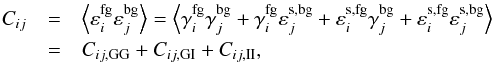 (8)where [i;j] = { + ; × }, γfg (γbg) is the cosmic shear acting on the foreground (background) object,
  is the cosmic shear correlation term, and
 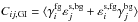 and
and  are the gravitational-intrinsic and the intrinsic-intrinsic correlation terms (see below). We note that the dominant term in Cij,GI is
  ; the other term,
  , is only expected to be non-negligible if there are long-range correlations in the gravitational tidal field (e.g., a dark matter filament along the line of sight), and can be ignored in most situations. In the case of a flat cosmology, the correlation functions are related to the density contrast power spectrum Pδ (e.g., see Bartelmann & Schneider 2001; Catelan et al. 2001)
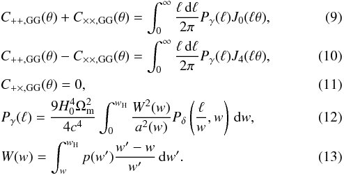
Here Pγ is the cosmic-shear power spectrum, J0 and J4 are Bessel functions of the first kind, p(w) is the probability of detecting a galaxy at comoving distance w, and wH is the comoving horizon distance.
To obtain relevant cosmological results from cosmic-shear measurements, it is important to understand each error source. From the theoretical point of view, an important error source is the contribution to the ellipticity correlation induced by the intrinsic alignment, Cij,GI + Cij,II.
2.2. Intrinsic alignment
As noted previously in computational (Heavens et al. 2000; Croft & Metzler 2000) and theoretical studies (Catelan et al. 2001), unlensed ellipticities need not be distributed isotropically. In particular, close pairs of galaxies may exhibit correlated ellipticities as a result of their mutual gravitational interaction and of an external gravitational potential.
The intrinsic alignment (IA) is the contribution to the observed galaxy ellipticity correlation, caused by the gravitational tidal field in which galaxies are placed. In the literature it is usually assumed (Catelan et al. 2001; Hirata & Seljak 2004) that the galaxy intrinsic ellipticity is frozen at the formation epoch. IA is classified according to the physical generating mechanism (Catelan et al. 2001), which is different according to the type of galaxy that the external gravitational field acts upon.
In elliptical galaxies, the external gravitational field stretches the galaxy shapes (Croft & Metzler 2000), partly determining their intrinsic ellipticities1. In contrast, in spiral galaxies the intrinsic ellipticity is related to their angular momentum, produced by the torque provided by the external gravitational field during galaxy formation and by projection effects (Heavens et al. 2000).
From a geometrical point of view (Hirata & Seljak 2004), the intrinsic correlation (for a second-order statistics, like the shear two-point correlation function) is made of two contributions: intrinsic-intrinsic (II) and gravitational-intrinsic (GI). The II contribution is the correlation of the unlensed ellipticities of two physically close2 source galaxies, generated by a correlation in the gravitational field felt by the galaxies (which is caused by their mutual interaction and by the external large-scale structure). In contrast, the GI correlation is the correlation between the observed ellipticities of two galaxies that are distant from each other, but angularly close in the sky view plane (Hirata & Seljak 2004). This correlation is caused by foreground mass inhomogeneities that produce two effects through the tidal field: they induce an intrinsic ellipticity in foreground galaxies through direct gravitational interaction and modify the observed ellipticities of background galaxies by means of gravitational lensing.
2.2.1. Elliptical galaxies
Elliptical galaxies are expected to be polarized by the external tidal field they are located in (Croft & Metzler 2000; Catelan et al. 2001),  Here εs is the galaxy ellipticity in the plane perpendicular to the line of sight, Uext represents the large-scale potential (at the galaxy formation epoch) associated with inhomogeneities of cosmological origin, and C is a constant that in principle could be determined by “a complete galactosynthesis model” (Catelan et al. 2001). Catelan et al. (2001) indirectly estimated this constant in a heuristic way by means of the relation
 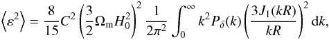 (16)where R = 1 h-1 Mpc is the characteristic scale over which a galaxy forms. An II alignment for elliptical galaxies has indeed been detected in numerical simulations (Croft & Metzler 2000) and observations (e.g. Pereira & Kuhn 2005; Agustsson & Brainerd 2006; Hirata et al. 2007; Faltenbacher et al. 2009; Joachimi et al. 2011).
For early-type galaxy samples with broad redshift distribution and for typical foreground mass inhomogeneities, the GI contribution is non-vanishing and is expected to be greater than that of the II contribution (Hirata & Seljak 2004). The GI term is due to the tidal effects of a mass overdensity on foreground galaxies, and the lensing effects of the same overdensity on background galaxies. Therefore, the relevant factor is the probability of observing an elliptical galaxy integrated along the line of sight from the mass overdensity to the horizon. In contrast, the relevant factor for the II term is the probability of observing a second galaxy at the same redshift as the first galaxy.
Finally, we note that according to this model, the GI alignment produces an anticorrelation of ellipticities (CGI< 0): the foreground elliptical galaxy physical (intrinsic) shape is stretched along the gravitational tidal field, whereas the background galaxy apparent shape is stretched perpendicular to it because of lensing (Hirata & Seljak 2004). For example, in a galaxy cluster, cluster members would be preferentially aligned radially, whereas the background galaxies would be seen preferentially tangentially.
2.2.2. Spiral galaxies
In spiral galaxies the II contribution is thought to be caused by the torque provided by the external tidal field during formation (Heavens et al. 2000; Catelan et al. 2001; Hirata & Seljak 2004, 2010). This contribution is to second order in the external tidal field because the tidal field first has to generate an anisotropic moment of inertia Iij (as in elliptical galaxies, the distribution of mass is expected to be elongated along the gravitational field gradient), and then to torque it (Peebles 1969; Doroshkevich 1970; White 1984). The torque provided by the external tidal field generates the angular momentum of the spiral proto-galaxy (this is similar to what we show in Appendix A, where we compute the torque generated by the external tidal field on an elliptical galaxy not aligned with it). One then needs to specify the correlation between the angular momentum and the galaxy ellipticity, for example by assuming zero thickness for the (circular) disk of the galaxy and considering the projection effects, as reported by Heavens et al. (2000). Finally, since a correlation in the tidal field induces a correlation in the angular momenta of close spiral galaxy pairs, the expected II power spectrum can be computed analytically, as shown by Hirata & Seljak (2004).
The II contribution for spiral galaxies is of higher order in the tidal field and thus should be lower than for ellipticals (Hirata & Seljak 2004). In addition, little GI contribution is expected for spiral galaxies (Hirata & Seljak 2004). At present, there is no clear observational evidence of IA in spiral galaxies (Hirata et al. 2007; Faltenbacher et al. 2009; Blazek et al. 2012).
In Appendix A we determine the rigid-body precession period of spiral galaxies, which is longer than the galaxy deformation time. This shows that no precession-driven mechanism for an alignment of spiral galaxies with the external tidal field can be devised.
3. Distribution function method
Even if galaxies are many-body systems, it might naïvely be thought that their alignment is driven by rigid-body motions (e.g., oscillations and precessions) under the effects of external gravitational forces. However, an analysis of the relevant time scales shows that rigid-body motions are much slower than those characterizing internal dynamics (Appendix A, see also Ciotti & Dutta 1994). This means that at least for IA purposes, the galaxy is best studied as a deforming body. In this section, we start from the hypothesis that galaxies are not subject to any intrinsic alignment during formation and that intrinsic alignment is entirely due to tidal fields at the observation time, to which galaxies react immediately. As shown in Sect. 4, this assumption leads to an extremely low IA, completely inconsistent with observations. This is an indirect proof that IA is driven by formation and merging.
The deformation of an elliptical galaxy subject to an external gravitational field can be modeled in a simplified way by studying the deformation of its equipotential surfaces (see Appendix B), and in a more complete manner, by means of the stellar distribution function. In both cases, we start with unperturbed spherical galaxies for simplicity and study the ellipticity induced by the external tidal field. The spherical assumption is quite strong, and it may not be straightforward to generalize our results to the case of an ensemble average of elliptical early-type galaxies. Nevertheless, since we are interested in an order-of-magnitude estimate, the spherical assumption is sufficient for our purposes.
3.1. General case
A galaxy is a complex many-body system, with a gravity-driven dynamics (Chandrasekhar 1942; Bertin 2000). In this context, an important tool is the stellar distribution function f⋆(x,ẋ,t), which is, essentially, the stellar density distribution in phase space. We also define (e.g., Bertin 2000) the (total) distribution function f = f⋆ + fDM as the sum of the stellar distribution function and the dark matter distribution function. We assume the collisionless Boltzmann equation and the Poisson equation: 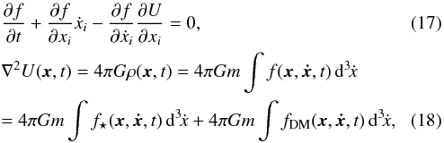 where m is the mean mass of a galaxy star (and of a DM “particle” as well). In the following, we use the King model (King 1966) for the stellar distribution function3
![\begin{eqnarray} f_\star(\vec x,\vec{\dot x},t)=\begin{cases}A\Big[\mathrm e^{-U(\vec x)/\sigma_v^2-\|\vec{\dot x}\|^2/(2\sigma_v^2)}-\mathrm e^{-E_\mathrm{tr}/\sigma_v^2}\Big]&E<E_\mathrm{tr},\\ 0&E\ge E_\mathrm{tr},\end{cases} \end{eqnarray}](/articles/aa/full_html/2015/03/aa25016-14/aa25016-14-eq52.png) (19)where
(19)where  is the single-star energy and σv is the stellar velocity dispersion, and we start from a spherical unperturbed (early-type) galaxy with potential U0. In other words, in the unperturbed galaxy the DM supplies the exact contribution to have the given potential U0 and the King distribution function for f⋆.
We take an external tidal potential and add it to the (unperturbed) galaxy potential, thus ignoring the changes in the galaxy potential induced by the deformation of the galaxy (for a similar not self-consistent approach, see Ciotti & Dutta 1994; see also Bertin & Varri 2008). As pointed out by Ciotti & Dutta (1994), it is possible to neglect the actual self-force of the galaxy because it decreases from the center of the galaxy (see, e.g., the potential (28)of the unperturbed self-field), whereas the external tidal force increases. Therefore, we take U = U0 + Utidal (see Bertin & Varri 2008; Varri & Bertin 2009 for a self-consistent approach applied to a globular stellar cluster). We take a weak external tidal field  and expand the stellar distribution function with respect to it
 ![\begin{eqnarray} f_\star&=& A\mathrm e^{-U_0(\vec x)/\sigma_v^2-\|\vec{\dot x}\|^2/(2\sigma_v^2)}\left(1-\sigma_v^{-2}\Phi_{ij}x_ix_j+\cdots\right)-A\mathrm e^{-E_\mathrm{tr}/\sigma_v^2}\notag\\[2mm] &=& f_\star^{(0)}+f_\star^{(1)}+\cdots,\\[2mm] f_\star^{(0)}&=&A\left(\mathrm e^{-U_0(\vec x)/\sigma_v^2-\|\vec{\dot x}\|^2/(2\sigma_v^2)}-\mathrm e^{-E_\mathrm{tr}/\sigma_v^2}\right),\\[2mm] f_\star^{(1)}&=&-\sigma_v^{-2}\Phi_{ij}x_ix_jA\mathrm e^{-U_0(\vec x)/\sigma_v^2-\|\vec{\dot x}\|^2/(2\sigma_v^2)}, \end{eqnarray}](/articles/aa/full_html/2015/03/aa25016-14/aa25016-14-eq59.png) where
where  is the tidal tensor and
 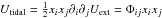 is the tidal field (potential).
This expansion is valid only inside the galaxy (Bertin & Varri 2008); in fact, even if the exponential can always be expanded (when | Utidal/σv | ≪ 1), this expansion is not granted to be meaningful unless the perturbed self-potential U0 + Utidal is not too different from the actual galaxy self-potential, U. This condition breaks down near the galactic boundaries because, as stated above, the galaxy self-potential decreases toward the boundaries, whereas the external tidal field increases (since Φij is traceless, the isopotential surfaces may not even be ellipses when | Utidal | ≃ | U0 |). From Eq. (1), changing integration variables to those of standard two-dimensional vectors, considering that  , and using Eq. (18), we obtain for the luminous quadrupole
 ![\begin{eqnarray} \label{eq:quadrupole-expansion} \tens Q_{ij}&=&\frac1{D_\mathrm{s}^2N}\int \left(f_\star^{(0)}+f_\star^{(1)}+\cdots\right)x_ix_j\,\mathrm d^3\!x\,\mathrm d^3\!\dot x\nonumber\\[2mm] &=&\tens Q_{ij}^{(0)}+\tens Q_{ij}^{(1)}+\cdots, \end{eqnarray}](/articles/aa/full_html/2015/03/aa25016-14/aa25016-14-eq68.png) (23)where Ds is the angular-diameter distance to the galaxy and N is the number of stars of the galaxy. The integration of Eq. (23)has to be carried out (i) in the region
(23)where Ds is the angular-diameter distance to the galaxy and N is the number of stars of the galaxy. The integration of Eq. (23)has to be carried out (i) in the region 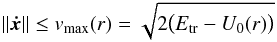 (24)because of the energy truncation in the distribution function and (ii) for ∥ x ∥ ≤ rmax<rtr, a condition that mimics a real weak-lensing measurement, where the integration in the luminous quadrupole is carried out based on a window function. The quantity rmax is chosen so as to avoid regions where the external tidal field becomes similar to or larger than the galactic field, that is, the condition | Utidal(rmax) | ≪ | U0(rmax) | holds (see discussion above). The zeroth order of the expansion of the luminous quadrupole
  is proportional to the identity matrix because the unperturbed galaxy field is spherical:
 ![\begin{eqnarray} \label{eq:Q-0} \tens Q_{ij}^{(0)}&=&\frac{(4\pi)^2 A}{3ND_\mathrm{s}^2}\Big(\mathcal F_1-\mathcal F_2\Big)\,\delta_{ij},~~~~~~~~~~~~~~~\\ \label{eq:F1} \mathcal F_1&=&\int_0^{r_\mathrm{max}}\mathrm dr\,r^4\mathrm e^{-U_0(r)/\sigma_v^2}\int_0^{v_\mathrm{max}(r)}v^2\mathrm e^{-v^2/(2\sigma_v^2)}\,\mathrm dv~~~\notag\\ &=&\sigma_v^2 \int_0^{r_\mathrm{max}}r^4 \mathrm e^{-U_0(r)/\sigma_v^2} \Bigg[-v_\mathrm{max}(r) \mathrm e^{-v_\mathrm{max}^2(r)/(2\sigma_v^2)}~~~\notag\\ &&\qquad\qquad\qquad\qquad\quad +\,\sigma_v\sqrt{\frac\pi2}\, \mathop{\mathrm{erf}}\left(\frac{v_\mathrm{max}(r)}{\sqrt2\sigma_v}\right) \Bigg]\,\mathrm dr,~~~~\\ \label{eq:F2} \mathcal F_2&=&\frac{\mathrm e^{-E_\mathrm{tr}/\sigma_v^2}}3\int_0^{r_\mathrm{max}}r^4\Big(v_\mathrm{max}(r)\Big)^3\mathrm dr. \end{eqnarray}](/articles/aa/full_html/2015/03/aa25016-14/aa25016-14-eq76.png) We use a galaxy logarithmic potential U0 (Fig. 1) to model the total mass distribution in a galaxy (luminous plus dark matter; see e.g. Bertin 2000; Koopmans et al. 2006)
We use a galaxy logarithmic potential U0 (Fig. 1) to model the total mass distribution in a galaxy (luminous plus dark matter; see e.g. Bertin 2000; Koopmans et al. 2006) 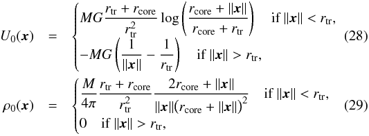 where M = 1011M⊙ is the galaxy mass, U0(rtr) = 0, rcore = 1 kpc is the core radius, and rtr = 25 kpc is the truncation radius. Throughout this paper we take for an elliptical galaxy σv ≃ [200 km s-1 and rmax = 10 kpc (see discussion above). We then obtain
  The first-order perturbation to the luminous quadrupole is
 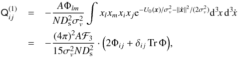 (32)where TrΦ = Φ11 + Φ22 + Φ33, and
 ![\begin{eqnarray} \label{eq:F3} \mathcal F_3&=&\sigma_v^2 \int_0^{r_\mathrm{max}}r^6 \mathrm e^{-U_0(r)/\sigma_v^2} \Bigg[-v_\mathrm{max}(r) \mathrm e^{-v_\mathrm{max}^2(r)/(2\sigma_v^2)}\notag\\ &&\qquad\qquad\qquad\qquad\qquad +\,\sigma_v\sqrt{\frac\pi2}\, \mathop{\mathrm{erf}}\left(\frac{v_\mathrm{max}(r)}{\sqrt2\sigma_v}\right)\Bigg]\,\mathrm dr\\ &\simeq& 4.9\times10^{-9}~{\rm Mpc^7\,(km\,s^{-1})^{3}}\notag. \end{eqnarray}](/articles/aa/full_html/2015/03/aa25016-14/aa25016-14-eq87.png) (33)From Eq. (2), considering that
(33)From Eq. (2), considering that  (spherical galaxy), we find for the complex ellipticity
 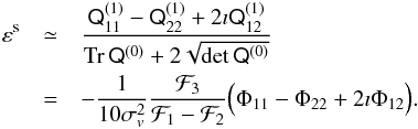 (34)Finally, we obtain the general expression for the ellipticity induced on a particular galaxy by an external tidal field. This expression can be factorized in two parts: one part only depends on the particular galaxy we are considering (its mass, its size, its self-field, and the velocity dispersion of its stars); the other part only depends on the tidal field, with the expected dependence (e.g., Catelan et al. 2001). The difference with Catelan et al. (2001) is that in Eq. (34)the external field is that acting at the moment of the light emission, and not that acting at the formation epoch. Comparing Eq. (34)with Eqs. (14)and (15), we obtain the analytic expression for the constant of proportionality appearing in Eqs. (14)and (15)
 (35)Equation (34)is the main result of this paper: it provides a direct way to estimate the intrinsic ellipticity of an early-type galaxy that is subject to an external tidal field.
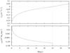 |
Fig. 1 Self-potential (28)and total mass distribution (29)of the unperturbed galaxy. The values used are rcore = 1 kpc, rtr = 25 kpc and M = 1011M⊙. The dashed vertical line indicates the truncation radius rtr. |
To better appreciate this result, consider a thin lens such as a galaxy cluster. In this case, we can write the lens shear as  (36)where the derivatives are given with respect to the physical coordinates, Ds, Dl and Dls are the angular distance of a source galaxy, of the lens, and between the lens and the source galaxy, respectively, and Lcl is the galaxy cluster typical size. Interestingly, the expression for γ has the same form as Eq. (34), that is, it depends on the same combination of second-order partial derivatives of the tidal tensor Φ. The constants involved, instead, are clearly different: in particular, for a typical galaxy cluster with Lcl ≃ 1 Mpc at zl = 0.5 and for a source at zs = 1 we find that the coupling constant between the shear γ and the tidal field is about −20C. As a result, in this context (for a galaxy cluster) we expect that the intrinsic alignment produced by the instantaneous tidal field is negligible.
3.2. Particular cases
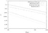 |
Fig. 2 Radial dependence of the intrinsic galaxy ellipticity in the particular cases (Keplerian and DM filament fields) considered in this paper, computed through the equipotential approximation (equi, see Appendix B) and through the distribution function formalism (f, see Sect. 3). Note the different radial dependence of the Keplerian (R-3) and the DM filament (R-2) cases; the equipotential approximation and the distribution function formalism yield the same radial dependence in the two cases, but different multiplicative factors (see the text for details). |
We now consider an external Keplerian field, that is, the potential generated by a second galaxy of mass Mext, assumed to be spherical and centered at R. The tidal acceleration and the tidal potential acting on a star of the first galaxy are 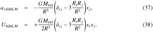 If we place the external galaxy at R = (R,0,0), using Eq. (34), we obtain (Fig. 2)
 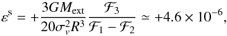 (39)where in the last step we used Mext = 1011M⊙ and R = 500 kpc. We note that εs = O(R-3).
We now examine a different case: the external field is generated by a dark matter (DM) filament, and the galaxy is outside it. We are considering a tidal field generated by an (infinite) linear distribution of matter along the line of sight 
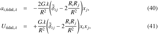 where R is the distance of the galaxy from the DM straight line (the filament),
  and λ is the linear mass distribution of the dark matter filament. Obviously, a3,tidal,λ = 0. We now need to estimate the quantity λ, the linear density of the DM filament. DM filaments are thought to extend between massive galaxy clusters (e.g., Springel et al. 2005). We therefore consider the number density of massive clusters and estimate the average distance dcl between two clusters. To do so, we use the cumulative distribution of galaxy clusters measured by Bahcall & Cen (1993):
 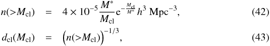 where M∗ = (1.8 ± 0.3) × 1014h-1M⊙ and h = 0.7. Setting Mcl = M∗ leads4 to
  (44)which is consistent with the typical value reported by Springel et al. (2005), that is, 100 Mpc. We assume that 34% of the mass in the Universe is concentrated in filaments, as the numerical results of Hoffman et al. (2012) indicates. We then have that
  (45)If we place the filament in such a way that it crosses the source plane at R = (R,0), with R = 500 kpc, and use Eq. (34), we obtain (Fig. 2)
  (46)We observe that in this case the dependence on the distance is εs = O(R-2).
4. Discussion
4.1. Comparison with literature
It is common (e.g., Joachimi & Bridle 2010; Joachimi et al. 2011) to consider the galaxy number density contrast-intrinsic ellipticity correlation, that is,  (47)where the correlation function only depends on the modulus of x because isotropy, δn is the galaxy number density contrast, and
  is the real part of the complex (intrinsic) ellipticity in a coordinate system with the real axis along the line connecting the two correlating points x0 and x, as in Eqs. (5)–(7). In contrast to Eqs. (5)and following, the correlation in Eq. (47)is carried on in the three-dimensional real space. We now define the Fourier transform
  of a function f(x) as
  (48)Since
 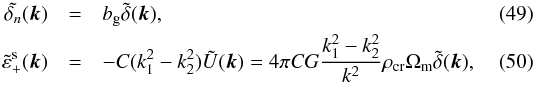 where bg is the galaxy bias and in the second equality of Eq. (50)we used Eq. (14), the Poisson equation and the relation
  (we neglect the three-dimensional Dirac delta in the origin). If we introduce the elliptical galaxy fraction fell (because only elliptical galaxies align in our model), we find
  (51)where Pδ(k,z) is the density contrast power spectrum at the galaxy redshift z and where we have approximated the term
  to unity. We may now consider Eqs. (6) and (19) of Joachimi et al. (2011), that is,
 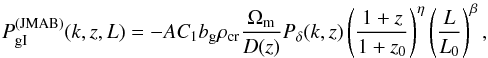 (52)where D(z) is the linear growth factor normalized to unity today, Pδ is the (nonlinear) power spectrum of the density contrast, z and L are the redshift and the absolute luminosity of the early-type galaxy, and the arbitrary reference values are z0 = 0.3 and L0, the latter corresponding to an absolute r-band magnitude of −22, passively evolved to z = 0. The parameters AC1, η, and β have been measured by Joachimi et al. (2011) for comoving transverse separations greater than 6 h-1 Mpc,
 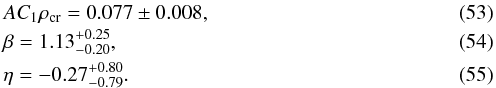 Comparing Eqs. (51)to (52)and neglecting the redshift and luminosity dependence, we obtain that Eq. (53)corresponds to the term
  (56)of Eq. (51), where we set fell = 1 because Joachimi et al. (2011) considered only early-type galaxies for the shape measurements. The result is clearly inconsistent. It is unlikely that this inconsistency is due to our use of the simple King model because the different approach adopted in Appendix B, where we do not make use of the stellar distribution function, yields similar results (cf. Eqs. (39), (46), (B.8)and (B.10)). Then, at least at large scales (rp> 6 h-1 Mpc), our model does not reproduce the observations.
The incompatibility of Eq. (56)with Eq. (53)means that the galaxy deformation due to the instantaneous external tidal field cannot yield the observed IA signal. A possible explanation is that the IA signal is caused by the galaxy formation process and/or its merging history. To obtain analytic results, these processes therefore need to be linked to the external tidal field. In particular, at least for the merging history, the velocity shear field needs to be considered because it was recently discovered (Hoffman et al. 2012; Libeskind et al. 2014; Lee & Choi 2015) that mergers preferentially occur along the velocity shear minor eigenvector. A detailed analysis of this process is beyond the aims of this paper.
4.2. Halo case
Until now, we have only considered the galaxy with its total (luminous plus dark) mass. We have stopped the integration of the luminous quadrupole at rmax<rtr. However, the ellipticity of the whole DM halo remains unclear. We remark that it is not obvious that Eq. (2)is the correct choice for the halo ellipticity because the halo luminous quadrupole cannot be measured in real surveys. For the same reason, it is unclear how to choose rmax, but for the condition | U0(rmax) | ≫ | Utidal(rmax) |. Still, it is interesting to consider the extreme case of a dark matter halo M = 2 × 10¹³M⊙, rtr = 560 kpc and σv = 250 km s-1, as found by Gavazzi et al. (2007) from an ensemble average over 22 massive halos. Even now, we obtain (taking rcore = 0.01·rtr and rmax = 0.80·rtr)
which is still almost a factor ~20 lower than the value of Eq. (53), that is, even if instantaneous tidal fields produce a greater IA on dark matter halos than on galaxies, the effect is still much too weak to account for the observed signal. Arguably, the galaxies observed by Joachimi et al. (2011) are, on average, less massive objects, and therefore the value of Eq. (57)should be taken as an upper bound. In addition, we stopped the integration near the halo boundaries (rmax = 0.80·rtr), and the resulting ellipticity is therefore greater than that we would obtain with a smaller rmax. This shows that our model is essentially inadequate to explain the observed amount of IA.
5. Conclusions
The exact origin of intrinsic alignment of galaxies is still unclear, and there are no analytic estimates of the amount of IA caused by different possible processes. We here support the standard view on IA (i.e., it is caused by formation and accretion processes) by a reduction ad absurdum. To arrive at this result, we estimated the amount of IA in elliptical galaxies due to an external instantaneous tidal field by considering the galaxy stellar distribution function and the luminous quadrupole. In addition, in Appendix A, we determined the typical oscillation time-scale for an elliptical galaxy modeled as a rigid body, subject to an external tidal field, and in Appendix B we determined the ellipticity of a galaxy (subject to an external instantaneous tidal field) in a different way by studying its equipotential surfaces. The main results are the following:
-
1.
The distribution function approach allows us to analyticallydetermine the dependence of the intrinsic ellipticity on the tidalfield, heuristically formulated by Catelanet al. (2001), in terms of theproperties of the galaxy (i.e., its mass, size, velocity dispersion,and stellar distribution function), Eqs. (34)and (35).
-
2.
The intrinsic alignment signal obtained when our model is applied to an elliptical galaxy is negligible with respect to the observed one (at least at large scales, >6 h-1 Mpc, Joachimi et al. 2011), cf. Eqs. (53)and (56). Thus one has to consider the galaxy formation process and/or its merging history.
-
3.
When our model is applied to the whole galaxy halo, the intrinsic alignment signal increases (but it is still inconsistent with the observed signal), Eq. (58).
The work we described here is a step toward a simple physical understanding of the bias introduced in weak-lensing measurements by IA. In the past, IA has been regarded as a source of concern for cosmic-shear measurements. More recently, it has been regarded as an opportunity to investigate the physical properties of galaxies, their DM halos, and their formation history. In this perspective, it is important to develop analytic models of IA, such as those presented here, to be able to interpret the results of future weak-lensing surveys. In this respect, a complete model of IA could even be used directly to reconstruct the local tidal field acting on elliptical galaxies.
The theoretical analysis could be improved by applying the techniques we presented (i.e., the stellar distribution function method) to the study of the formation and accretion processes, in order to determine their contributes to the IA signal. It would also be interesting to study the contribution to IA due to continuously applied tidal fields (instead of only considering the tidal field acting at the emission epoch, as we have did here), and the evolution of IA with redshift.
Online material
Appendix A: Rigid-body approximation
In this appendix we compare the time scale of motions of galaxies modeled as rigid bodies with the time scale of their internal dynamics. In particular, we consider the (rigid) oscillations of elliptical galaxies (a similar analysis has been carried out in Ciotti & Giampieri 1997) and the precession of spiral galaxies. We show below that internal dynamics is much faster than rigid-body dynamics, thus confirming the results of Ciotti & Dutta (1994) for elliptical galaxies.
Appendix A.1: General case
We assume that the distribution of mass of the galaxy only depends on the elliptical radius  and that its principal axes are aligned with the coordinate axes:
  where r1, r2 and r3 are the semi-axes of the ellipsoid (ρ = 0 for
  ). Then the inertia tensor is
  (A.3)where δ is the Kronecker delta, and we placed the center of mass of the galaxy in the origin. With this definition, the moment of inertia
  along the unit vector
  is
is  (A.4)For an elliptical mass distribution whose principal axes are parallel to the coordinate axes we obtain
  The potential energy W of a body subject to the action of the external field Uext(x) (whose Laplacian is null in the region occupied by the galaxy) is (Jackson 1998)
  where M and
  are the mass and the quadrupole tensor of the body. For an elliptical mass distribution with principal axes parallel to the coordinate axes we obtain
  (A.10)
Appendix A.2: Elliptical galaxies: oscillation period
For a Keplerian potential, the galaxy energy is  (A.11)Without loss of generality, let
  be diagonal and let θ and ϕ be the angles between the
  axis and R and between the
  axis and
  , in a spherical coordinate system (see Fig. A.1). In other words, we consider a coordinate system whose axes are parallel to the principal axes of the galaxy.
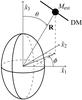 |
Fig. A.1 Spherical coordinate system adopted in the text, Keplerian (Mext) and DM filament cases. |
Having kept diagonal, we have to rotate the tidal tensor. Considering that  , we find
  (A.12)We can in principle determine the oscillation equations of the galaxy via the Euler-Lagrange equations, using the correct kinetic energy expression. This approach leads to complex equations and therefore we assume that (i) the elliptical distribution of mass is prolate (i.e., r1 = r2 = req<r3), from which I11 = I22 = Ieq and
  ; and (ii) there are no initial intrinsic rotation (
 ) or precession motions; there could be only nutation (
 ). Using the Euler-Lagrange equations, we then obtain
  (A.13)We explicitly note that this equation is not self-consistent: in fact, in principle it should be completed with the equations of the relative motion between the galaxy center of mass and the monopole. However, we are not interested in a complete treatment of the problem, but only in an analytic estimate of the time scale of an oscillation. Therefore we assume, without clarifying the physical mechanism that would permit this, that the relative position between the external monopole and the galaxy is fixed, and that only the orientation of the galaxy can vary. With these assumptions, Eq. (A.13)is sufficient to describe the dynamics of the system. To obtain the time scale of an oscillation, we make the small-angle approximation (θ ≪ 1) and recall that
  (prolate galaxy), obtaining the pendulum equation. Considering that the components of I and are of the same order of magnitude, we find that the period tosc,M of an oscillation is
  (A.14)We remark that Eq. (A.14)is reminiscent of the expression of the free-fall time tff ∝ (Gρ)− 1/2 ∝ tosc,M × (D/ 2R)3/2, being D the diameter of the galaxy. Using the values adopted here for the external mass Mext = 1011M⊙ and for the distance R = 500 kpc, the period is tosc,M ≃ 1.0 × 10¹¹ yr, which is greater than the age of the Universe5 (the numerical integration of Eq. (A.13)is in accordance with the approximate result).
This period has to be compared with the time scale on which the shape of a galaxy changes, because of the external gravitational field. A rough estimate of this is the time necessary for a star to travel across the galaxy (e.g., Fleck & Kuhn 2003)  (A.15)where σv is the stellar velocity dispersion and D is the diameter of the galaxy. For D ≃ 40 kpc and σv ≃ 200 km s-1, we obtain tcross,ell ≃ 2 × 10⁸ yr ≪ tosc,M. In other words, an elliptical galaxy, not aligned with the gravitational tidal field, deforms itself before completing a rigid oscillation.
If we consider a DM filament along the  axis, using Eq. (41), we can write the galaxy energy as
  (A.16)where ℓ′ is an arbitrary constant introduced to have an adimensional logarithmic argument, and
  . As before, we rotate the coordinate frame in such a way that be diagonal6 (see Fig. A.1), we use spherical coordinates and assume that the galaxy is prolate, that there are no proper rotation nor precession motions, and that the position of the galaxy is fixed. We then obtain
  (A.17)Using the same approximations as before and Eq. (45), we may estimate the period of a small rigid oscillation of the galaxy
  (A.18)which in the case considered throughout the paper (R = 500 kpc) corresponds to 5.0 × 10⁹ yr. This is shorter than the period of oscillation found in the Keplerian case, but nevertheless greater than tcross,ell. We therefore have to drop the rigid-body approximation and deepen the description of elliptical galaxies to account for the internal degrees of freedom, as done in Sect. 3 and Appendix B.
Appendix A.3: Spiral galaxies: precession period
The key feature that distinguishes spiral galaxies from elliptical ones is the dominance of ordered motions over chaotic ones, that is, the characterizing presence of the angular momentum. If we place a rigid body with an angular momentum in an external field, it starts precessing. In this subsection we estimate the precession period for a spiral galaxy, taken as a rigid body.
The precession period tprec of a rotating rigid body is  (A.19)where L is the angular momentum of the spiral galaxy, θ is the angle between L and the external force, and τ(θ) is the amount of the momentum of the external force. In spiral galaxies the luminous mass distribution is very different from that of the dark matter; in our calculation we can detach the two contributions because the DM distribution is (approximately) spherical and does not generate a torque on the visible mass, in which we are interested. To determine the total stellar angular momentum L⋆, we can use the rigid-body formula L⋆ = I⋆ 33ω⋆. In spiral galaxies stars at different distances from the center of the galaxy have different angular velocities (ω⋆ = ω⋆(ℓ), where ℓ is the distance from the symmetry axis of the spiral). Therefore it is sensible to use a weighted angular velocity
  , defined as
  (A.20)where Σ⋆(ℓ) is the projected stellar surface density at distance ℓ from the spiral symmetry axis and v⋆(ℓ) is the stellar tangential velocity. In spiral galaxies, the stellar tangential velocity is approximately constant, v⋆(ℓ) ≃ v⋆, and the stellar column density follows an exponential law with length scale ℓ0, Σ⋆(ℓ) = Σ0exp( − ℓ/ℓ0). We then obtain
  (A.21)Using this expression in Eqs. (A.13)and (A.17), we find for an oblate galaxy (r3<r1 = r2 = req)
 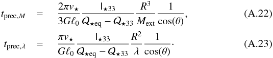 Assuming v⋆ = 200 km s-1 and ℓ0 = 10 kpc, we obtain
  Therefore the time scale is longer than or similar to the age of the Universe, and it is also longer than the deformation time of spiral galaxies (similarly to that of the elliptical galaxy).
Appendix B: Equipotential approximation
In Sect. 3 we have obtained the expression of the intrinsic ellipticity of an early-type galaxy subjected to an external tidal field. To do so, we have calculated the luminous quadrupole, making use of the stellar distribution function. In this appendix we present another approach, which is less complete but has the advantage of having a clear and simple physical understanding. In particular, we model the deformation of the galaxy by means of the equipotential surfaces of the total gravitational potential. In this approach, we “assume[s] that the local galaxy density is produced approximately by stars near their zero-velocity surfaces” (Ciotti & Dutta 1994). As in Sect. 3, (i) we start with an unperturbed spherical galaxy; (ii) we take an external tidal potential and add it to the (unperturbed) galaxy potential, thus ignoring the changes in the galaxy potential induced by the deformation of the galaxy (see also Ciotti & Dutta 1994; Bertin & Varri 2008); and (iii) we assume that the galaxy immediately reacts to a change of the external gravity field by modifying its shape accordingly (see Sect. 3 for details).
Appendix B.1: General case
In the absence of external fields, the galaxy potential U0 obeys the Poisson equation  (B.1)where ρ0 is the unperturbed galaxy mass distribution. We now introduce a (weak) external potential Uext, so that U0 → U = U0 + Uext. The introduction of the external field changes the equipotential surfaces of the galaxy. Given a volume
  enclosed by a particular equipotential surface
  at energy E0 of the unperturbed potential, we consider the corresponding equipotential surface
  for U
for U (B.2)The energy shift δE is chosen in such a way that the mass inside the surface does not change:
  (B.3)A Taylor expansion of the right-hand side of Eq. (B.3)for low δE − Uext gives
  (B.4)Since ρ0 has spherical symmetry, ρ0 and ∇U0 are uniform on
  , and we finally obtain
  (B.5)If Uext ≡ Utidal = Φijxixj, that is, the external potential is a tidal one, δE is equal to zero, because Φij is traceless and has spherical symmetry.
We use the galaxy logarithmic potential of Eq. (28). If we introduce an external tidal potential, the equipotential surface becomes an ellipsoid (see Fig. B.1). We place the galaxy center at the origin and align the coordinate axes along the eigenvectors of the tidal tensor Φij. Then, we can evaluate the deviation from the circular shape of a particular equipotential surface with radius rmax<rtr by expanding to first order its semi-axis variations δi in Eq. (B.2),  (B.6)We kept for generality δE, even if it vanishes for an external tidal field. Equation (B.6)allows us to compute the intrinsic ellipticity of a particular isophotal of a galaxy subject to a tidal field as observed along any direction. For this, we just have to project an ellipsoid with semi-axes rmax + δ1, rmax + δ2 and rmax + δ3 along the line of sight. For example, if the ellipsoid is observed along , we would have from Eq. (3)
 (B.7)
(B.7)
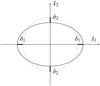 |
Fig. B.1 Schematic representation of the deformation of a two-dimensional contour of an equipotential surface. The dotted line is the unperturbed contour, the solid line the perturbed contour. In the tidal approximation, the variations along the positive and negative directions are the same. |
Appendix B.2: Particular cases
For the Keplerian tidal field (38), placing the external spherical galaxy at R = (R,0,0), using (B.7), and assuming rmax,rtr ≪ R, we obtain (Fig. 2) 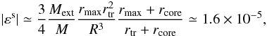 (B.8)where in the last step we used Mext = 1011M⊙, rmax = 10 kpc and R = 500 kpc. We note that εs = O(R-3), and that the ellipticity becomes lower for inner equipotential surfaces.
For an external DM filament directed along the line of sight and distant R = 500 kpc from the galaxy, if we assume7 (B.9)we obtain from Eqs. (41), (45)and (B.7)(Fig. 2)
  (B.10)We observe that in this case the dependence on the distance is εs = O(R-2); again, inner equipotential surfaces have lower ellipticity.
The values obtained through the equipotential approximation (B.8)and (B.10)are higher than those obtained through the distribution function method (39)and (46); the reason is that with the equipotential approximation we only consider an outer isopotential surface, which is more deformed than the inner ones. Instead with the distribution function method, more realistically, we are “weighting the ellipticities of the isophotes” of the galaxy from its center to rmax. Equations (B.8)and (B.10)have the same dependence on R as was found with the distribution function method (see Fig. 2).
In cosmic-shear measurements, the II signal is usually suppressed by excluding pairs of galaxies from the analysis that are thought to be physically close (with their physical distance estimated from photometric redshifts and angular distance in the sky). However, the assumption that only physically close galaxies have II alignment might not hold because the II alignment could arise also in far away galaxies if there are long-range correlations in the gravitational field (e.g., those associated with a dark matter filament, the typical length scale of which is numerically estimated as 100 h-1]Mpc by Springel et al. 2005; see also Mandelbaum et al. 2006; Lee 2004; Hirata et al. 2007). Moreover, since the distance between galaxies is estimated from photometric redshifts, galaxies thought to be physically distant may actually be physically close as a result of errors in the photometric redshift estimates.
An important point to keep in mind is that the large-scale structure is strongly time-dependent and that the mean high-mass-cluster distance changes with time (Springel et al. 2005). Here, we are considering the local Universe, that is, regions where the redshift is much lower than unity.


Acknowledgments
We wish to thank Giuseppe Bertin and Benjamin Joachimi for invaluable suggestions and very useful discussions, which significantly improved the paper. We also thank the anonymous referee for his or her helpful suggestions concerning the presentation of this paper. G.C. thanks Malegori’s family (“Franca Erba” scholarship) and BCC Carugate e Inzago Bank (“Gildo Vinco” award) for supporting his studies.
References
- Agustsson, I., & Brainerd, T. G. 2006, ApJ, 644, L25 [NASA ADS] [CrossRef] [Google Scholar]
- Bahcall, N. A., & Cen, R. 1993, ApJ, 407, L49 [NASA ADS] [CrossRef] [Google Scholar]
- Bartelmann, M., & Schneider, P. 2001, Phys. Rep., 340, 291 [NASA ADS] [CrossRef] [Google Scholar]
- Bertin, G. 2000, Dynamics of Galaxies (Cambridge: Cambridge University Press) [Google Scholar]
- Bertin, G., & Varri, A. L. 2008, ApJ, 689, 1005 [NASA ADS] [CrossRef] [Google Scholar]
- Blazek, J., Mandelbaum, R., Seljak, U., & Nakajima, R. 2012, JCAP, 5, 41 [Google Scholar]
- Catelan, P., Kamionkowski, M., & Blandford, R. D. 2001, MNRAS, 320, L7 [NASA ADS] [CrossRef] [Google Scholar]
- Chandrasekhar, S. 1942, Principles of Stellar Dynamics (Chicago: The University of Chicago Press) [Google Scholar]
- Ciotti, L., & Dutta, S. N. 1994, MNRAS, 270, 390 [NASA ADS] [CrossRef] [Google Scholar]
- Ciotti, L., & Giampieri, G. 1997, Celest. Mech. Dyn. Astron., 68, 313 [Google Scholar]
- Croft, R. A. C., & Metzler, C. A. 2000, ApJ, 545, 561 [NASA ADS] [CrossRef] [Google Scholar]
- Doroshkevich, A. G. 1970, Astrofizika, 6, 581 [Google Scholar]
- Faltenbacher, A., Li, C., White, S. D. M., et al. 2009, RA&A, 9, 41 [Google Scholar]
- Fleck, J.-J., & Kuhn, J. R. 2003, ApJ, 592, 147 [NASA ADS] [CrossRef] [Google Scholar]
- Fu, L., Semboloni, E., Hoekstra, H., et al. 2008, A&A, 479, 9 [NASA ADS] [CrossRef] [EDP Sciences] [Google Scholar]
- Gavazzi, R., Treu, T., Rhodes, J. D., et al. 2007, ApJ, 667, 176 [NASA ADS] [CrossRef] [Google Scholar]
- Heavens, A., Refregier, A., & Heymans, C. 2000, MNRAS, 319, 649 [NASA ADS] [CrossRef] [Google Scholar]
- Heymans, C., & Heavens, A. 2003, MNRAS, 339, 711 [NASA ADS] [CrossRef] [Google Scholar]
- Heymans, C., White, M., Heavens, A., Vale, C., & van Waerbeke, L. 2006, MNRAS, 371, 750 [NASA ADS] [CrossRef] [Google Scholar]
- Hirata, C. M., & Seljak, U. 2004, Phys. Rev. D, 70, 063526 [NASA ADS] [CrossRef] [Google Scholar]
- Hirata, C. M., & Seljak, U. 2010, Phys. Rev. D, 82, 049901 [NASA ADS] [CrossRef] [Google Scholar]
- Hirata, C. M., Mandelbaum, R., Ishak, M., et al. 2007, MNRAS, 381, 1197 [NASA ADS] [CrossRef] [Google Scholar]
- Hoffman, Y., Metuki, O., Yepes, G., et al. 2012, MNRAS, 425, 2049 [NASA ADS] [CrossRef] [Google Scholar]
- Jackson, J. D. 1998, Classical Electrodynamics, 3rd edn. (John Wiley & Sons) [Google Scholar]
- Jauzac, M., Jullo, E., Kneib, J.-P., et al. 2012, MNRAS, 426, 3369 [Google Scholar]
- Jing, Y. P. 2002, MNRAS, 335, L89 [NASA ADS] [CrossRef] [Google Scholar]
- Joachimi, B., & Bridle, S. L. 2010, A&A, 523, A1 [NASA ADS] [CrossRef] [EDP Sciences] [Google Scholar]
- Joachimi, B., Mandelbaum, R., Abdalla, F. B., & Bridle, S. L. 2011, A&A, 527, A26 [NASA ADS] [CrossRef] [EDP Sciences] [Google Scholar]
- Kaiser, N. 1992, ApJ, 388, 272 [NASA ADS] [CrossRef] [Google Scholar]
- Kaiser, N., Squires, G., & Broadhurst, T. 1995, ApJ, 449, 460 [NASA ADS] [CrossRef] [Google Scholar]
- Kilbinger, M., Fu, L., Heymans, C., et al. 2013, MNRAS, 430, 2200 [NASA ADS] [CrossRef] [Google Scholar]
- King, I. R. 1966, AJ, 71, 64 [Google Scholar]
- King, L., & Schneider, P. 2002, A&A, 396, 411 [NASA ADS] [CrossRef] [EDP Sciences] [Google Scholar]
- Koopmans, L. V. E., Treu, T., Bolton, A. S., Burles, S., & Moustakas, L. A. 2006, ApJ, 649, 599 [NASA ADS] [CrossRef] [Google Scholar]
- Lee, J. 2004, ApJ, 614, L1 [NASA ADS] [CrossRef] [Google Scholar]
- Lee, J., & Choi, Y.-Y. 2015, ApJ, 799, 212 [NASA ADS] [CrossRef] [Google Scholar]
- Libeskind, N. I., Knebe, A., Hoffman, Y., & Gottlöber, S. 2014, MNRAS, 443, 1274 [NASA ADS] [CrossRef] [Google Scholar]
- Mandelbaum, R., Hirata, C. M., Ishak, M., Seljak, U., & Brinkmann, J. 2006, MNRAS, 367, 611 [NASA ADS] [CrossRef] [Google Scholar]
- Miralda-Escudé, J. 1991, ApJ, 380, 1 [NASA ADS] [CrossRef] [Google Scholar]
- Peebles, P. J. E. 1969, ApJ, 155, 393 [NASA ADS] [CrossRef] [Google Scholar]
- Pereira, M. J., & Kuhn, J. R. 2005, ApJ, 627, L21 [NASA ADS] [CrossRef] [Google Scholar]
- Refsdal, S. 1964, MNRAS, 128, 295 [NASA ADS] [CrossRef] [MathSciNet] [Google Scholar]
- Schramm, T., & Kayser, R. 1995, A&A, 299, 1 [NASA ADS] [Google Scholar]
- Seitz, C., & Schneider, P. 1997, A&A, 318, 687 [NASA ADS] [Google Scholar]
- Springel, V., White, S. D. M., Jenkins, A., et al. 2005, Nature, 435, 629 [NASA ADS] [CrossRef] [PubMed] [Google Scholar]
- Tenneti, A., Mandelbaum, R., Di Matteo, T., Feng, Y., & Khandai, N. 2014, MNRAS, 441, 470 [NASA ADS] [CrossRef] [Google Scholar]
- Troxel, M. A., & Ishak, M. 2014 [arXiv:1407.6990] [Google Scholar]
- Varri, A. L., & Bertin, G. 2009, ApJ, 703, 1911 [NASA ADS] [CrossRef] [Google Scholar]
- White, S. D. M. 1984, ApJ, 286, 38 [NASA ADS] [CrossRef] [Google Scholar]
All Figures
|
Fig. 1 Self-potential (28)and total mass distribution (29)of the unperturbed galaxy. The values used are rcore = 1 kpc, rtr = 25 kpc and M = 1011M⊙. The dashed vertical line indicates the truncation radius rtr. |
| In the text | |
|
Fig. 2 Radial dependence of the intrinsic galaxy ellipticity in the particular cases (Keplerian and DM filament fields) considered in this paper, computed through the equipotential approximation (equi, see Appendix B) and through the distribution function formalism (f, see Sect. 3). Note the different radial dependence of the Keplerian (R-3) and the DM filament (R-2) cases; the equipotential approximation and the distribution function formalism yield the same radial dependence in the two cases, but different multiplicative factors (see the text for details). |
| In the text | |
|
Fig. A.1 Spherical coordinate system adopted in the text, Keplerian (Mext) and DM filament cases. |
| In the text | |
|
Fig. B.1 Schematic representation of the deformation of a two-dimensional contour of an equipotential surface. The dotted line is the unperturbed contour, the solid line the perturbed contour. In the tidal approximation, the variations along the positive and negative directions are the same. |
| In the text | |
Current usage metrics show cumulative count of Article Views (full-text article views including HTML views, PDF and ePub downloads, according to the available data) and Abstracts Views on Vision4Press platform.
Data correspond to usage on the plateform after 2015. The current usage metrics is available 48-96 hours after online publication and is updated daily on week days.
Initial download of the metrics may take a while.