| Issue |
A&A
Volume 575, March 2015
|
|
|---|---|---|
| Article Number | A51 | |
| Number of page(s) | 15 | |
| Section | Stellar atmospheres | |
| DOI | https://doi.org/10.1051/0004-6361/201424998 | |
| Published online | 20 February 2015 | |
Quest for the lost siblings of the Sun ⋆,⋆⋆
1 Lund ObservatoryDepartment of Astronomy and Theoretical Physics Box 43 221 00 Lund Sweden
e-mail: This email address is being protected from spambots. You need JavaScript enabled to view it.
; This email address is being protected from spambots. You need JavaScript enabled to view it.
; This email address is being protected from spambots. You need JavaScript enabled to view it.
2 Leiden Observatory, University of Leiden, PB 9513, 2300 RA Leiden, The Netherlands
Received: 16 September 2014
Accepted: 19 November 2014
Abstract
Aims. The aim of this paper is to find lost siblings of the Sun by analyzing high resolution spectra. Finding solar siblings will enable us to constrain the parameters of the parental cluster and the birth place of the Sun in the Galaxy.
Methods. The solar siblings can be identified by accurate measurements of metallicity, stellar age and elemental abundances for solar neighbourhood stars. The solar siblings candidates were kinematically selected based on their proper motions, parallaxes and colours. Stellar parameters were determined through a purely spectroscopic approach and partly physical method, respectively. Comparing synthetic with observed spectra, elemental abundances were computed based on the stellar parameters obtained using a partly physical method. A chemical tagging technique was used to identify the solar siblings.
Results. We present stellar parameters, stellar ages, and detailed elemental abundances for Na, Mg, Al, Si, Ca, Ti, Cr, Fe, and Ni for 32 solar sibling candidates. Our abundances analysis shows that four stars are chemically homogenous together with the Sun. Technique of chemical tagging gives us a high probability that they might be from the same open cluster. Only one candidate – HIP 40317 – which has solar metallicity and age could be a solar sibling. We performed simulations of the Sun’s birth cluster in analytical Galactic model and found that most of the radial velocities of the solar siblings lie in the range −10 ≤ Vr ≤ 10 km s-1, which is smaller than the radial velocity of HIP 40317 (Vr = 34.2 km s-1), under different Galactic parameters and different initial conditions of the Sun’s birth cluster. The sibling status for HIP 40317 is not directly supported by our dynamical analysis.
Key words: stars: abundances / stars: fundamental parameters / solar neighborhood
Based on observations made with Nordic Optical Telescope at La Palma under programme 44-014. Based on observations made with ESO VLT Kueyen Telescope at the Paranal observatory under program me ID 085.C-0062(A), 087.D-0010(A), and 088.B-0820(A). Based on data obtained from the ESO Science Archive Facility under programme ID 078.D-0080(A), 080,A-9006(A), 082.C-0446(A), 082.A-9007(A), 083,A-9004(B), and 089.C-0524(A).
Full Table 2 is only available at the CDS via anonymous ftp to cdsarc.u-strasbg.fr (130.79.128.5) or via http://cdsarc.u-strasbg.fr/viz-bin/qcat?J/A+A/575/A51
© ESO, 2015
1. Introduction
It is commonly thought that stars are born within clusters and that the majority of embedded clusters do not survive longer than 10 Myr (Lada & Lada 2003). The Sun, like most stars, could have been born in a cluster. The stars that were born with the Sun are called solar siblings. Finding them will enable us to determine the birthplace of the Sun (Portegies Zwart 2009) and to better understand the importance of radial mixing in shaping the properties of disk galaxies (Bland-Hawthorn et al. 2010). It should be possible to identify them by obtaining accurate measurements of their kinematics, metallicities, elemental abundances, and ages.
Based on implications for the formation and morphology of the solar system and presence of short-lived radioactive nuclei in meteorites, the possible birth environment of the Sun has been probed by several studies. As discussed by Portegies Zwart (2009), a parent cluster could contain 103−104 stars, and the size of the proto-solar cluster was between 0.5 and 3 pc. The same characteristics of the parent cluster were found by Adams (2010). He also points out that a massive supernova explosion happened about 0.1–0.3 pc from the Sun. Wielen et al. (1996) found that the Sun has travelled outwards by about 2 kpc from the birthplace over the past 4.6 billion years. Comparing the cosmic abundance standard that was obtained by measuring early B-type stars in solar neighbourhood with the solar standard, Nieva & Przybilla (2012) also claim that the Sun has migrated outwards from its birthplace in the inner disk at 5–6 kpc Galactic distance over its lifetime to the current position. The radial migration of stars might be caused by transient spiral arms at corotation: churning (Sellwood & Binney 2002).
Using simulations, Portegies Zwart (2009) find that about 10–60 solar siblings could still be within 100 pc of the Sun if assuming the parental cluster consisting of ~103 stars. Following the previous analysis, Brown et al. (2010) simulated the orbits of the stars in the Sun’s birth cluster rather than tracing the Sun’s orbit back over the whole lifetime in an analytic Galactic potential. The first potential candidate for a solar sibling was found based on their simulated phase-space distribution of the siblings. When taking the perturbation from spiral arms in Galactic potential into account, Bobylev et al. (2011) find two interesting stars by constructing their Galactic orbits and analysing the parameters of encounter with solar orbit. Another potential candidate was found by considering the chemical compositions, age, and kinematics properties of FGK stars from the Geneva-Copenhagen Survey Catalogues (Holmberg et al. 2009) by Batista & Fernandes (2012). One more potential candidate was found in a search for solar siblings using HARPS (Batista et al. 2014). However, Mishurov & Acharova (2011) argue that the solar siblings are unlikely to be found within 100 pc of the Sun, because an unbound open cluster is dispersed in a short period of time under the perturbation of the spiral gravitational field. Then, the members of cluster are scattered over a very large portion of the Galactic disk after 4.6 Gyr of dynamical evolution. In addition to the radial migration, the original kinematical information has been modified as a result of perturbations of the spiral arms and central bar. They also point out that we still have a chance to find the solar siblings in the solar vicinity if the parental cluster has ~104 stars (Mishurov & Acharova 2011). The first real solar sibling HD 162826 that satisfies both chemical and strictly dynamical conditions was found by Ramírez et al. (2014). This is encouraging and strengthens our ability to find the lost siblings of the Sun.
Since the original kinematical information of a star may be lost under the Galactic dynamic evolution, it will not be the first option for identifying the solar siblings. The chemical information, on the other hand, is preserved in the form of elemental abundances in individual stars. To reconstruct dissolved star clusters, Freeman & Bland-Hawthorn (2002) first proposed the technique of chemical tagging based on understanding chemical signatures that members of an open cluster are chemically homogeneous. The homogeneity of abundances in open clusters and moving groups have been demonstrated by recent studies (De Silva et al. 2007a,b, 2009; Pancino et al. 2010). A pair-wise metric, which quantifies the differences in chemical signatures between different clusters and the stars within a given cluster, has been defined by Mitschang et al. (2013). This metric was applied to more than 30 open clusters with good measurement of elemental abundances, and they find that it is effective ( 9% of the total sample of stars, see also Mitschang et al. 2014) in detecting the members of clusters.
In Sect. 2, we present our sample of sibling candidates. We describe observations and the process of data reductions in Sect. 3. Both stellar parameters and elemental abundances are determined in Sect. 4. Our algorithm of chemical tagging is explained in Sect. 5. In Sect. 6, we give constraints on metallicity, stellar age, and elemental abundances and find that only one candidate could be solar sibling in our sample, and in Sect. 7 we give dynamical analysis of a previously identified star. Finally, conclusions are drawn in Sect. 8.
2. Selecting solar sibling candidates
Solar sibling candidates were selected following the same methods and steps as in Brown et al. (2010). Assuming solar siblings have almost the same orbit as the Sun and taking the varying distance into account, the upper limit on the proper motion value can be obtained in their simulations. Stars within 100 pc of the Sun are selected. The predicted proper motion versus parallax phase space was used as a first selection of solar sibling candidates in the Hipparcos catalogue (van Leeuwen 2007). The exact selection criteria were  (1)where ϖ and μ are the parallax and proper motion of the stars, respectively, and σϖ is the precision of the parallax. Since the Sun and solar siblings formed together in the parent cluster, the siblings should have about the same age as the Sun. Inspection of stellar isochrones shows that for solar metallicity, a star with a colour of B − V ≤ 0.4 is too young to be a solar sibling. Finally, 57 candidates were selected from the Hipparcos catalogue using two constraints. In this work, high resolution spectra of 33 of 57 candidates are analysed. The basic properties of the 33 sibling candidates, shown in Fig. 1, were collected from the Strömgren photometric and Hipparcos catalogues (van Leeuwen 2007; Olsen 1983, 1994), respectively. The data are listed in Table 1.
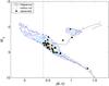 |
Fig. 1 Colour–magnitude diagram showing the absolute magnitude MV versus. B − V. The contour plot shows the distribution of the stars in the Hipparcos catalogue with σϖ/ϖ ≤ 0.1 and σB − V ≤ 0.05 (van Leeuwen 2007). The spectra of the 33 sibling candidates are indicated with triangles. The solid line shows an isochrone with the age (5 Gyr) and metallicity of the Sun (Demarque et al. 2004). The vertical dashed line indicates our cut-off at B − V = 0.4. |
Basic data for our solar sibling candidates.
3. Observations and data reductions
Observations were carried out with two telescopes for 26 sibling candidates, while the spectra of seven stars were collected from the ESO archive (Table 1). Eighteen of the candidates were observed at the Nordic Optical Telescope (NOT) using the fibre-fed Echelle Spectrograph (FIES) on January 10–12 in 2012. A solar spectrum was also obtained by observing the sky at daytime. The wavelength range of the spectra is 370–730 nm, with a resolution R ~ 67 000 and a signal-to-noise ratio (S/N) > 150/pix for most of the spectra. All the spectra were reduced using the FIEStool1 pipeline. The pipeline includes the following steps to reduce the observed frame: subtracting bias and scattered light, dividing by a normalized two-dimensional flat field, extracting individual orders, and finding a wavelength solution and applying it. Finally, all individual spectral orders are merged into a one-dimensional spectrum.
Spectra for 12 stars were observed using the UVES spectrograph (Dekker et al. 2000) on the VLT 8-m telescope between 2011 and 2012 in service mode. Using image slicer #3 and a 0.3′′ slit width, a resolution R ~ 110 000 was reached in the red arm. The spectra were recorded on three CCDs with wavelength coverages 376–498 nm (blue CCD), 568–750 nm (lower red CCD), and 766–946 nm (upper red CCD). We found that the average S/N of one spectrum in three wavelengths is greater than 160 for all the spectra. The data were reduced with the UVES pipeline. Spectra of 4 of these 12 stars had already been observed with FIES. Although it has been noted that using different spectrographs does not introduce significant systematic differences in the derived stellar parameters (Santos et al. 2004), it is still worth doing a further analysis to test for systematic differences (see Sect. 4.3.2).
The spectra for seven stars extracted from the ESO archive were observed between 2007 and 2010 with FEROS on the ESO 2.2-m telescope (Kaufer et al. 1999). We checked that the S/N values for these spectra are higher than 100. Since the ESO archive offers reduced 1D spectra with a wavelength range of 350–920 nm, we used these spectra for our study. Radial velocities for all spectra were measured by cross-correlation with the solar synthesis spectrum based on the IRAF2 task XCSAO. The spectra were also shifted to rest wavelength for radial velocity with the IRAF task DOPCO. Their radial velocities are listed in Table 3 including their standard deviation.
4. Spectral analysis
For our spectral analysis, we used Spectroscopy Made Easy (SME, Valenti & Piskunov 1996; Valenti & Fischer 2005) to determine the stellar parameters for each star, namely, the effective temperature (Teff), surface gravity (log g), metallicity ([Fe/H]), elemental abundances, and micro-turbulence (vmic). SME uses the Levenberg-Marquardt (LM) algorithm to optimize stellar parameters by fitting observed spectra with synthetic spectra. The LM algorithm combines gradient search and linearization methods to determine parameter values that yield a chi-square (χ2) value close to the minimum. Initial stellar parameters (Teff, log g, and [Fe/H]) and atomic line data are required to generate a synthetic spectrum. In addition to specified narrow wavelength segments of the observed spectrum, SME requires line masks in order to compare with synthetic spectrum and determine velocity shifts, and continuum masks that are used to normalize the spectral segments. The homogeneous segments and masks are created to fit all of our solar sibling candidates.
In SME the model atmospheres are interpolated in the precomputed MARCS model atmosphere grid (Gustafsson et al. 2008), which have standard composition. The MARCS grid in SME includes Teff = 2500–8000 K in steps of 100 K from 2500 to 4000 K and 250 K between 4000 and 8000 K, log g = −0.5 to 5.0 in steps of 0.5, and metallicities between –5.0 to 1.0 in variable steps.
4.1. The line list
The elemental abundance derived from a single spectral line is directly proportional to the oscillator strength (log gf) for that line. Therefore, as Bensby et al. (2003) point out, the highest priority is to find homogeneous and accurate log gf values, so we have had to make a decision between laboratory and astrophysically determined log gf values. In addition, the elemental abundance can also be altered by blends. In Table 2, we list 110 clean iron (80 Fe i and 20 Fe ii) lines selected from the Bensby et al. (2003) and Gaia-ESO compiled line list (Heiter et al., in prep.). The α-elements (Mg, Si, Ca, Ti), iron peak elements (Ni, Cr), and sodium and aluminium lines were also selected from those two catalogues. All our clean lines were examined on the Sun’s spectrum.
4.2. The methods for estimating stellar parameters
Our spectroscopic analysis requires that we estimate six free parameters: Teff, log g, [Fe/H], vmic, vmac, and vsini. We have developed two procedures to efficiently and accurately determine these parameters through multi-step processes.
4.2.1. Procedure 1: Purely spectroscopic parameters
Atomic line data.
In this procedure, the initial values for Teff, log g, and [Fe/H] are input (the specifics of which are described in Sects. 4.3 and 4.4 for the solar sibling candidates and benchmark stars, respectively). An initial value for vmic was obtained using the relation given in Jofre et al. (2014b), which was derived for stars in the Gaia-ESO survey. Initial values for vsini were determined by measuring the difference in the full width at half maximum (FWHM) of atomic and telluric lines in the spectrum. This was done using Spectra Visual Editor software (priv. comm. with Blanco-Cuaresma). Finally, the initial vmac value was set to 3.0 km s-1 for all stars. Since we are solving for several free parameters simultaneously, there is a degeneracy in the effect of each parameter on the strength of the absorption lines in the spectra. Thus, we have developed a multi-step process to effectively break these degeneracies. The iterative procedure (hereafter procedure 1) follows these steps:
-
1.
only vmac is free, while other parameters are fixed;
-
2.
only vsini is free, and fixed vmac comes from step 1;
-
3.
only [Fe/H] is free, and fixed vsini is from step 2;
-
4.
both vmic and vsini are free, and fixed [Fe/H] comes from step 3;
-
5.
repeat steps 1 to 4 with updated parameters (vmic and vsini) until vmac, vmic and vsini converge;
-
6.
Teff, log g, and [Fe/H] are free, and the other fixed parameters are from step 5;
-
7.
repeat steps 1 to 6 with updated parameters (Teff, log g, and [Fe/H]) until all six parameters reach convergence.
4.2.2. Procedure 2: Using parallax estimates
Stellar parameters of sibling candidates.
It has been shown that analysis, which computes stellar parameters using purely spectroscopic means, can lead to erroneous results. For example, Bensby et al. (2014) identified that for dwarf stars with log g> 4.2, enforcing ionization equilibrium between Fe i and Fe ii lines does not yield accurate log g estimates. Our analysis could also suffer from such systematic effects. Thus, we have also developed a second procedure (hereafter procedure 2) in which we determine log g using parallax estimates for the stars.
We compute log g using the following equation:  (2)where V, ϖ, M, and B.C. are the apparent magnitude, parallax, stellar mass, and bolometric correction, respectively. Since the stars are located in the Local Bubble (Lallement et al. 2003), we assume that the extinction is negligible (comparing with Nissen et al. 2014). Flower (1996) expressed the bolometric corrections as a function of Teff and found that all luminosity classes appear to follow a unique Teff − B.C. relation. We thus used this relation, utilizing the corrected coefficients from Torres (2010) to obtain B.C. for our stars. The stellar mass and age of each star require fitting isochrones using our estimated values for Teff, log g, and [Fe/H]. Thus, we must iterate until the input stellar parameters and output mass and age converge.
Procedure 2 is defined by the following approach. Firstly, using procedure 1, Teff and [Fe/H] were computed by fixing log g in SME. Then, the mass and age were obtained through fits to the Yonsei-Yale isochrones (Demarque et al. 2004) by maximising the probability distribution functions, as described in Bensby et al. (2011). Substituting these values of Teff and mass into Eq. (2), new log g values were calculated. We then returned to the first step in procedure 1 and recomputed Teff and [Fe/H], holding log g fixed. These new values were then used to fit to the isochrones to get new estimates of mass and age. We iterated until convergence between the log g, mass, and age estimates. The final values for Teff, log g, and [Fe/H] were obtained when the stellar parameters converge and the average differences of stellar ages and masses from two iterations are less than 0.1 Gy and 0.01 solar mass, respectively.
4.3. Stellar parameters for solar sibling candidates
4.3.1. Initial stellar parameters
Initial effective temperatures for the stars were determined using both Strömgren (uvby) and UBV photometry (Olsen 1983, 1994; Table 1). The Strömgren photometric system is specially designed to measure the physical properties of the stellar atmospheres, and the colour (b − y) is very sensitive to the effective temperature. The calibration of Teff versus (b − y) − c1 − [ Fe/H ] from Alonso et al. (1996b, their Eq. (9)) was used. The uvby data is taken from Olsen (1983, 1984, 1994). However, some of our candidates were not included in those catalogues. Since the Hipparcos catalogue offers B − V for all of our stars, the relationship of (B − V) − Teff − [ Fe/H ] from Alonso et al. (1996b, their Eq. (2)) was also used to calculate Teff. The standard deviation for this calibration of Teff is 130 K, which implies a precision of 2.2% at the Sun’s temperature (5777 K). For the Strömgren Teff, the standard deviation is 110 K.
Alonso et al. (1996b) found that an error of 0.3 dex in [Fe/H] implies a mean error of 1.3% in Teff. For our solar sibling candidates, it is safe to assume that all of them have solar metallicity. This is supported by the small variation in [Fe/H] obtained from our abundance analysis. The average of the two effective temperatures was used as our initial guess for Teff.
Initial gravities were determined using Eq. (2)and the photometric estimated for Teff. We furthermore assumed that all the candidates have solar metallicity and age (~4.6 Gyr). Since the effective temperatures and absolute magnitudes (MV) of candidates are obtained in the previous section, we can obtain the masses for all candidates by interpolating Teff and MV within isochrones Yonsei-Yale isochrones (Demarque et al. 2004).
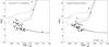 |
Fig. 2 a) HR diagram for the sample when a)log g is based on Fe i-Fe ii ionization equilibrium and b) when log g is based on Hipparcos parallaxes. Four isochrones at solar metallicity and four different ages (1, 3, 5, and 6 Gyr) according to the Yonsei-Yale models (Demarque et al. 2004) are also shown. |
4.3.2. Best stellar parameters
All stellar parameters derived using procedures 1 and 2 are given in Table 3. In Fig. 2, we show a comparison of the result that stellar parameters from each procedure in the H-R diagram. As can be seen in Fig. 2a, some stars with log g> 4.2 appear to fall in regions not occupied by the isochrones, when stellar parameters were derived using purely spectroscopic means. On the other hand, when we used log g derived using the parallax, we saw improvements in each star’s location in the H-R diagram (Fig. 2b). This is in part because we used the isochrones to derive our parallax gravities. Even though the isochrones have their own associated uncertainties (corresponding to uncertainties in stellar evolution theory), we expect the systematic effect on the derived parallax gravities to be less than 0.15 dex (see Eq. (2)). Thus, for the remainder of our analysis we adopt the stellar parameters derived using procedure 2.
In Fig. 2b it should be noticed that one star – HIP 89825 – has unexpected large log g and is far below the isochrones. The reason could be that we got the wrong bolometric correction for this star. As Torres (2010) points out, bolometric corrections become less reliable for cooler stars and break down completely for M dwarfs. Thus the obtained bolometric correction of HIP 89825, which is a typical M dwarf, could be far from the real one. It also should be mentioned that assumptions of solar metallicity and age were made in order to derive the initial Teff and stellar mass. However, HIP 89825 has much lower metallicity than does the Sun. All suggests that a unreliable log g from the parallax was estimated. However, log g from pure spectroscopic approach has a reasonable value as shown in Fig. 2a. In this case, the stellar parameters from pure spectroscopic approach were used to determine the elemental abundances for this star.
Although our iron line list was slightly different for the FIES and UVES spectra because of different wavelength observations, we found that four out of the five stars, including the Sun, observed by both the FIES and UVES instruments have quite similar outputs in stellar parameters. The mean differences in stellar parameters are within the estimated uncertainties. This suggests that our analysis gives the same results independently of the spectra and their resolutions. Outputs of vmic, vmac, and vsini for two spectra of a star, HIP 9405, are not far from each other. However, they have totally different values in Teff, log g, and [Fe/H]. Comparing two spectra, it clearly shows that the two spectra come from two stars. Recently, a study has concluded that HIP 9405 belongs to a binary system (Frankowski et al. 2007). It is highly possible that two spectra come from two companion stars, respectively. We cannot identify which spectrum comes from our sibling candidate. Thus, we exclude this star from the rest of our analysis. We carefully inspected all spectra and found that the spectra of HIP 56798 and HIP 25358 have clear double line signatures. They could be companion stars of binaries. It could bring larger uncertainties than our given typical errors on stellar parameters caused by near-by line blending. It also should be noticed that the stellar parameters of fast rotational stars (vsini> 30 km s-1) might suffer larger uncertainties than the typical errors.
4.4. Estimating systematic uncertainties
To determine the systematic errors in our derived stellar parameters from Procedure 2, we applied our analysis to several standard stars for which accurate stellar parameters have been estimated by other means.
4.4.1. Gaia benchmark stars
Recently, a set of reference stars have been created for calibration purposes in the Gaia mission. For these benchmark stars, Teff and log g are well determined independently of spectroscopy. Effective temperatures of benchmark stars are directly determined from angular diameters and bolometric fluxes. Surface gravities are also directly measured from the stellar mass and radius, which are calculated based on angular diameter and parallax, while the metallicity of each benchmark star has been derived through spectroscopic (Jofre et al. 2014a).
In the current work, the Sun and four benchmark stars (listed in Table 4) are used to test our methods, derive systematic errors and fix the linelist. These benchmark stars are very similar to the Sun in metallicity (Δ [ Fe/H ] < ± 0.1) and cover the same Teff and log g range as our sibling candidates. Ten high SNR spectra of four benchmark stars and the Sun collected from the UVES archives (Dekker et al. 2000), NARVAL3, HARPS (Mayor et al. 2003), and UVES-POP library (Bagnulo et al. 2003) were analysed.
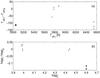 |
Fig. 3 a)Teff,r − Teff,p vs. Teff,p, where Teff,r represents the recommended effective temperature. Teff,p is the best-determined effective temperature from our methodology. Five symbols stand for the five benchmark stars, while two (or three) of the same symbol indicates that spectra obtained with different instruments were analysed. It is the same for the log gr and log gp that are shown in panel b). |
4.4.2. Estimating systematic errors in our stellar parameters
Although Teff and log g are well determined for the benchmark stars, we recalculated them using photometry and astrometry data to emulate our exact methodology for our solar sibling candidates. Figure 3 shows the difference between the recommended values listed in Table 4 (given by Teff,r and log gr) and those derived by our methods. It was found that the mean difference in Teff, log g, [Fe/H], and vsini and their standard deviation are –67 ± 40 K, –0.08 ± 0.06 dex, –0.05 ± 0.03 dex, and 0.2 ± 1.3 km s-1, respectively. It should be noticed that the typical uncertainties of the recommended Teff and log g are about 50 K and 0.02 dex for the benchmark stars, respectively. The random errors of log g obtained from distances and temperatures are between 0.04 to 0.06 dex. It is consistent with the scatter of mean difference of log g. Considering these systematic errors and possible sources of uncertainty on atmospheric model and atomic line data, the systematic errors in the stellar parameters were estimated to be δTeff = 67 K, δlog g = 0.08 dex, and δvsini = 0.2km s-1.
Although the recommended metallicities were determined from high-resolution spectra, it might suffer a large uncertainty. It is known that [Fe/H] depends on both Teff and log g. We can simulate the distribution of errors of [Fe/H] by iterating different Teff and log g values. A two-dimensional grid was created with varying Teff and log g. Since we have estimated errors of Teff and log g from our benchmark stars analysis, we assumed that initial values of Teff and log g vary within 3σ in steps of 50 K and 0.05, respectively. The spectra of the Sun, ϵ Eri, and HIP 51581 were used to calculate Δ[Fe/H], the difference between the newly output [Fe/H] and those obtained from procedure 2. Figure 4 shows how Δ[Fe/H] significantly correlates with ΔTeff for one of three stars. On the other hand, the trend between Δ[Fe/H] and Δlog g is hardly detected, because log g is sensitive to Fe II rather than Fe I, and most of the selected lines are Fe I in our line list.
Because no significant correlation between Δ[Fe/H] and Δlog g was found, the change in [Fe/H] responding to the error of log g is much smaller than with ΔTeff. It was also found that the maximum uncertainty of [Fe/H] caused by the typical error in vsini is 0.01 dex within our three tested stars. The change in [Fe/H] is still very small between 0.01–0.02 dex, if we vary the vmic by 0.1 km s-1. We then could simply use the root sum square of all changes to calculate the total uncertainty in [Fe/H]. Finally, uncertainties of [Fe/H] are between 0.04 to 0.06 dex for spectra with different S/N. It is consistent with the mean difference of [Fe/H] between what is recommended and our studies for benchmark stars. The maximum uncertainty of 0.06 dex will be regarded as the systematic error of measurement in metallicity.
4.5. Ages
The age of each star was determined during the fits to the isochrones in Procedure 2, as described in Sect. 4.2.2. The most probable age is determined from the peak of the age probability distribution, 1σ lower and upper age limits are obtained from the shape of the distribution. Stellar masses were also determined in a similar manner. Both ages and masses are reported in Table 5. It clearly shows that most of solar sibling candidates have younger ages than does the Sun in Fig. 2.
It is possible that the probabilistic age determinations used in our analysis suffer from systematic biases mainly caused by sampling the isochrone data points (Nordström et al. 2004). Age degeneracy around the zero-age main sequence or at the turn-off could also induce systematic effects because of complex isochrones. The Bayesian approach proposed by Jørgensen & Lindegren (2005) was used to cope with these problems. To find out whether possible systematic biases exist in our probabilistic determinations, we used the da Silva et al. (2006) PARAM web interface4 Bayesian-based method of estimating the stellar ages. Comparing our ages with the PARAM determined ages, the average difference is –0.1 Gyr, with a standard deviation 0.6 Gyr, which is much smaller than the typical uncertainties which are of the order of 1 Gyr. This suggests that the determined ages of our sample are reliable.
Stellar parameters for the Sun and four benchmark stars used to develop our methodology.
4.6. Abundance analysis
We obtained abundances by fitting the selected absorption lines for each element. During the abundance analysis, we left corresponding elemental abundance (e.g., [Na/H]) free, while the stellar parameters were kept fixed. The average ratio ANa (the absolute abundance relative to the total number density of atoms) was output from SME. The solar elemental abundance pattern taken from Grevesse et al. (2007) was used as a template for stellar abundances, in order to obtain the abundance ratio [Na/H]. The abundance ratios with respect to Fe (i.e. [X/Fe] in standard notation) were also calculated and are shown in Table 6. We measured abundances for Na, Mg, Al, Si, Ca, Ti, Cr, and Ni using either neutral or both neutral and singly ionized lines, as listed in Table 2. For comparison, we also derived solar abundances using the same line list and the stellar parameters derived from our solar spectrum in Sect. 4.3.2. For the solar sibling candidates observed by FIES and FEROS, we determined the elemental abundances (see Table 6) relative to solar values using the spectrum of sky at daytime. For the spectra of targets observed with UVES, the elemental abundances relative to solar values were determined using the solar spectrum reflected by the Moon. Some studies point out that systematic biases in solar abundance analysis could be introduced by aerosol and Rayleigh-Brillouin scattering filling up the day sky solar spectrum (Gray et al. 2000) and using different spectrographs (Bedell et al. 2014). To find out if possible biases exist in our solar abundances, we measured the equivalent widths (EWs) of two solar spectra from both FIES and UVES for all iron lines and found that the average difference of two solar EWs is –1.9 ± 4.6 mÅ. Comparing with typical uncertainties in elemental abundances (see Sect. 4.7), we ignored the systematic error caused by the average difference of EWs.
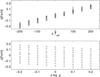 |
Fig. 4 Sensitivity of [Fe/H] to changes in stellar parameters for the Sun. A significant correlation between Δ[Fe/H] and ΔTeff exists, while the trend between Δ[Fe/H] and Δlog g is hardly detected. |
4.7. Errors in elemental abundances
There are many possible sources of uncertainty in our derived abundances. These can include continuum placement, line blending, and errors in stellar parameters and in atomic data (log gf). Since we performed a differential abundance analysis relative to the Sun, errors due to uncertainties in the log gf values cancel to first order. Errors due to continuum placement and line blending are estimated by SME. SME gives us a typical error less than 0.01 dex. In Sect. 4.4.2 the uncertainties of stellar parameters were estimated to be σTeff = 40 K, σlog g = 0.06 dex, and σ[ Fe/H ] = 0.03 dex. The uncertainties in the elemental abundances associated with these, for three stars (Sun, ϵ Eri, and HIP 51581), are given in Table 7. We found that errors in the elemental abundances do not correlate with the errors on the parameters. The total uncertainty was therefore derived by taking the square root of the quadratic sum of the different errors. The average values of the total uncertainties for all elements are between 0.03 and 0.05 dex.
Stellar masses, absolute magnitudes, and ages of solar-sibling candidates.
Elemental abundances of solar-sibling candidates.
Errors in the abundances due to the uncertainties in stellar parameters: Teff ± 40 K, log g ± 0.06 dex, [Fe/H] ± 0.03 dex.
5. Chemical tagging
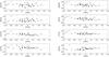 |
Fig. 5 Elemental abundance ratios [X/Fe] relative to Fe. Dashed lines indicate solar values. |
Chemical tagging is potentially a powerful tracer of the dispersed substructures of the Galactic disk (Freeman & Bland-Hawthorn 2002; De Silva et al. 2009). Here we used a chemical tagging method introduced by Mitschang et al. (2013). This method has been developed to find dispersed clusters in large-scale surveys. Here we give a brief summary of the method. A metric (δC) was defined as 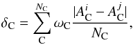 (3)where NC is the number of measured abundances,
  and
and  are individual abundance ratios of element C with respect to Fe relative to solar for stars i and j, respectively, and AC is the ratio of Fe to H when element C is Fe. As Mitschang et al. (2013) recommend, ωC, which represents a weighting factor for an individual species was fixed at unity. Here, δC is the mean absolute difference between any two stars across all measured elements. The probability that a particular pair of stars are members of the same cluster based on their δC can be estimated from a empirical probability function (PδC, see Mitschang et al. 2013 for more details). Mitschang et al. (2013) suggest a method of verifying a group of potential coeval stars from large data sets. We use a similar procedure adapted to our special case. Firstly, δC and PδC listed in Table 6 were calculated based on nine elements (Na, Mg, Al, Si, Ca, Ti, Cr, Ni, Fe) between any one solar-sibling candidate and the Sun, because the Sun is a standard star in this work and is assumed to have come from a dissolved open cluster. We picked up all calculated pairs with a probability greater than a given confidence limit. The high confidence limit Plim = 85% is set in order to reduce contamination stars from other clusters. Secondly, all remaining sibling candidates that make up the pairs from the above step were re-evaluated. The pairs of two stars that have probability PδC< 85% were cut out in this step. Finally, as Mitschang et al. (2013) suggest, the cluster-detection confidence, Pclus, can be evaluated using the mean of δC for the sibling candidates that remain.
The five potential solar siblings found in this way, HIP 21158, HIP 24232, HIP 40317, HIP 73600, and HIP 107528, have δC ≤ 0.042. For this group of stars, pairs of any two stars were made and their δC and PδC were re-evaluated. Four sibling candidates (HIP 21158, HIP 24232, HIP 40317, and HIP 73600) were identified as cluster stars. This means that five stars, including the Sun, might come from a dissolved cluster. This is consistent with the expected mean number of stars (~4.8) in each group that can be detected by the given confidence limit Plim = 85% (Mitschang et al. 2013). Finally, the cluster detection confidence is Pclue = 91%, which corresponds to the mean of δC = 0.034.
6. Potential solar siblings
Twelve of our stars have iron abundances consistent with the solar value within systematic and random uncertainties in [Fe/H]. Comparison with the age of the Sun (~4.6 Gyr) and relevant isochrones shows that 4 out of these 12 stars, HIP 10786, HIP 21158, HIP 40317, and HIP 51581, are consistent with the solar age within 1σ. They are thus potential candidates.
In addition to the constraints from [Fe/H] and stellar age, chemical signatures can help us to explore the probability that we have found true solar siblings. The members of a stellar aggregate formed in a common proto-cluster are found to have a high level of chemical homogeneity (De Silva et al. 2007b,a; Pancino et al. 2010). The abundance ratios with respect to Fe of all elements, as a function of [Fe/H], are shown in Fig. 5. We found flat trends for the α elements with abundances close to the solar abundances; however, [Al/Fe] and [Ni/Fe] show an increasing abundance for [Fe/H] < 0. We found that 15 out of 32 stars have PδC larger than 68 % according to the chemical tagging method. Only four sibling candidates, HIP 21158, HIP 24232, HIP 40317, and HIP 73600, are tagged by our method with a cluster detection confidence greater than 90%.
In these two sets of potential siblings, two key targets, HIP 21158 and HIP 40317, have ages and abundances in [X/Fe] similar to the Sun. This is consistent with the prediction of Mitschang et al. (2013) that 50% of the detections with members from other star aggregates give a high level confidence limit (Plim = 85). It should not be surprising that two of the four tagged cluster stars are not solar siblings.
Although our results on [Fe/H] and stellar age allow that two stars, HIP 10786 and HIP 51581, are possible solar siblings, they might not have formed from the same proto-cluster gas as the Sun because of the low probability (<68%) of a member of the stellar aggregate (see Table 6). HIP 24232 and HIP 73600 was tagged as a cluster star in Sect. 5 by the chemical tagging. However, the stellar ages of the stars are at least 2 Gyr younger than the Sun. According to the location of these two stars in the H–R diagram, HIP 24232 is a typical subgiant star and HIP 73600 is a main sequence star close to the turnoff point. The determined young ages could be trusted. For these two stars we also estimated an age of 1.6 ± 0.6 Gyr (HIP 24232) and 2.0 ± 1.6 Gyr (HIP 73600) by using the PARAM database (da Silva et al. 2006). It implies that they might be the members of a later dissolved cluster that has solar abundances.
One key target (HIP 21158) has been mentioned by both Brown et al. (2010) and Batista & Fernandes (2012) as a potential solar sibling. Although HIP 21158 is tagged as a cluster star based on [X/Fe] abundance ratios, it appears to have +0.1 offset in [Mg/H] and metallicity. Ramírez et al. (2014) also find that it has super-solar abundances for all their measured elements. The inconsistency in HIP 21158 might imply that [Fe/H] should be given a weighting factor in Eq. (3) that is larger than 1. The age derived for HIP 21158 (5.2 Gyr) is slightly older than the Sun and consistent with several other studies of the stellar ages (Feltzing et al. 2001; Takeda et al. 2007; Casagrande et al. 2011). Another key target, HIP 40317, has perfectly solar abundances both in [X/Fe] and [X/H] ratios. Two stellar ages were obtained for this star, because two observations were made using two different telescopes. Although the stellar ages suffer large uncertainty because it is a main sequence star, the mean difference in age between this star and the Sun is less than 1.2 Gyr. This suggests that it could be a lost sibling of the Sun.
7. Properties and dynamics of the solar siblings
7.1. Rotational velocity of star
According to the previous studies of stellar rotational revolution, the decline in rotation with age caused by angular momentum loss through the ionized wind is well established from observations of clusters (Soderblom 2010; Mamajek & Hillenbrand 2008). Nearly all of the velocities of F, G, and K stars fall below 12 km s-1 (Radick et al. 1987) by the age of the Hyades (~625 Myr; Perryman et al. 1998). If we assume that all solar-sibling candidates are born in the same parent cluster, they might have more or less the same rotation rate as that of the Sun after about a 4.6 Gyr decline in rotation. Since the projected rotational velocity of HIP 40317 from our synthesis fitting is 0.8 km s-1, the star could very well have the same rotational velocity as the Sun (depending on inclination sini).
7.2. Radial velocity of the Sun’s siblings
Initial conditions of the Sun’s birth cluster.
The solar abundances and age of HIP 40317 make this star a highly potential candidate for being one of the lost siblings of the Sun; however, the barycentric radial velocity of HIP 40317 is equal to 34.2 km s-1. By performing N-body simulations, we study the evolution in the Galaxy of the already extinct Sun’s birth cluster. Our aim is to conclude whether nearby solar siblings may exhibit high radial velocities. At the beginning of the simulations, the parental cluster of the Sun obeys a spherical Plummer density distribution function (Plummer 1911), together with a Kroupa IMF (Kroupa 2001). The initial mass (Mc) and radius (Rc) of the Sun’s birth cluster were set according to the values suggested by Portegies Zwart (2009). The initial conditions used in the simulations are listed in Table 8.
Galactic parameters of the Milky Way.
The Milky Way was modelled as an analytical potential consisting of an axisymmetric component, together with a central bar and spiral arms. We adopted the same Galactic model as Martínez-Barbosa et al. (2015) where the axisymmetric part of the Galaxy is modelled by using the potential of Allen & Santillan (1991), which consists of a bulge, disk, and a dark matter halo. The parameters that describe the axisymmetric component of the Milky Way are listed in Table 9.
The central bar of the Milky Way was modelled with a Ferrers potential (Ferrers 1877), which is described by a density distribution of the form: 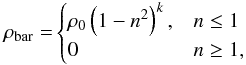 (4)where ρ0 represents the central density of the bar, which is related to its mass Mbar, and n2 determines the shape of the potential of the bar. On the Galactic plane, n2 = x2/a2 + y2/b2, with a and b its semi-major and semi-minor axes, respectively. The parameter k measures the degree of concentration of the bar. In the simulations, we use k = 1 (Romero-Gómez et al. 2011). In addition to the former parameters, we assume that the bar rotates as a rigid body with constant pattern speed Ωbar. The values of the mass, semi-major axis, axis ratio, and pattern speed of the bar are listed in Table 9 and were set to fit the observations made by the COBE/DIRBE survey (see Pichardo et al. 2004, 2012; Romero-Gómez et al. 2011).
The spiral structure of the Milky Way is represented as a periodic perturbation of the axisymmetric component of the Galaxy. The potential associated to this perturbation is given by  (5)where Asp is the amplitude of the spiral arms, R and φ are the galactocentric cylindrical coordinates, RΣ and m are the scale length and number of spiral arms, respectively, and g(R) is the function that defines the locus shape of spiral arms. We use the same shape factor as Antoja et al. (2011):
 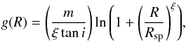 (6)where ξ is a parameter that measures how sharply the change from a bar to a spiral structure occurs in the inner regions. Here, ξ → ∞ produces spiral arms that begin forming an angle of ~90° with the line that joins the two starting points of the locus, thus we chose ξ = 100 (Antoja et al. 2011). Likewise, Rsp is the separation distance of the beginning of the spiral shape locus, and tani is the tangent of the pitch angle. Additionally, we assume that the spiral arms of the Galaxy rotate as a rigid body with pattern speed Ωsp. The values of the former parameters are listed in Table 9, and they correspond to the best fit to the Perseus and Scutum arms of the Milky Way (see Antoja et al. 2011).
In the numerical simulations the Sun’s birth cluster is evolved under the influence of its self-gravity, stellar evolution, and the external gravitational field generated by the analytical model of the Galaxy. The motion of the stars due to their self-gravity was computed by the HUAYNO code (Pelupessy et al. 2012). The motion of the stars under the external tidal field of the Milky Way was computed by a sixth-order rotating BRIDGE (Martínez-Barbosa et al. 2015). Additionally, we used the SeBa code (Portegies Zwart & Verbunt 1996; Toonen et al. 2012) to model the stellar evolution of the stars. We assumed a solar metallicity (Z = 0.02 or [ Fe/H ] = 0) for the Sun’s birth cluster. HUAYNO, the sixth-order rotating BRIDGE and SeBa were coupled through the AMUSE framework (Portegies Zwart et al. 2013).
The initial phase-space coordinates of the Sun’s birth cluster centre of mass (xcm, ycm, vxcm, vycm) were obtained by evolving the orbit of the Sun backwards in time, taking the uncertainty in the Sun’s current position and velocity into account, as is shown in Martínez-Barbosa et al. (2015). The orbit integration backwards in time gives a distribution of all the possible positions and velocities of the Sun at its birth, so we chose one position and velocity from this distribution to be the initial phase-space coordinates of the Sun’s birth cluster center of mass. This procedure was followed for different bar and spiral arm parameters.
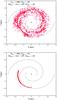 |
Fig. 6 Final distribution on the Galactic plane of solar siblings when Mc = 804.6 M⊙ and Rc = 3 pc. The final phase-space coordinates of the solar siblings depend on the configuration of the Galactic potential. Top: the Sun’s siblings are dispersed on the Galactic disk. Bottom: the solar siblings are located in a specific region on the Galactic disk. The dashed black lines represent the potential of the spiral arms at the end of the simulation. |
Once the Sun’s birth cluster is located at coordinates (xcm, ycm, vxcm, vycm), it is evolved forwards in time during 4.6 Gyr. We used a time step of 0.5 Myr and 0.16 Myr for HUAYNO and the sixth-order rotating BRIDGE, respectively. These values give a maximum energy error of 10-7 during the entire simulation. We carried out 1071 simulations in total, assuming different bar and spiral arm parameters in the Galactic model, as well as different initial masses and radii of the Sun’s birth cluster.
Depending on a given combination of bar and spiral arm parameters, the current distribution on the xy plane of the solar siblings could be highly dispersed or not, as can be seen in Fig. 6. Since all the bar and spiral arms parameters listed in Table 9 are equally probable, the final distribution of the solar siblings shown in this figure is equally plausible. In the case of a highly dispersed distribution, the difference between the maximum and minimum positions of the solar siblings (ΔR) can be higher than 3 kpc. Additionally, the siblings of the Sun may exhibit a broad range of azimuths. An example of a high dispersed distribution of solar siblings is shown in the top panel of Fig. 6. The set of Galactic parameters that produce high dispersion on the current distribution of the solar siblings are
-
when m = 2: 27 ≤ Ωsp ≤ 28km s-1 kpc-1 and Asp ≥ 900[ km s-1 ] 2 kpc-1;
-
when m = 4: Ωsp ≥ 18km s-1 kpc-1; ∀Asp.
We found that the high dispersion in the current phase-space coordinates of the solar siblings does not depend on Mc and Rc. For the specific case shown in the top panel of Fig. 6, the solar siblings span a range of radii between 2.9 and 11.6 kpc (ΔR = 8.6 kpc). Hereafter, we call the high dispersed distribution of solar siblings as the high dispersion case.
The current distribution on the xy plane of the solar siblings could also exhibit a small radial and angular dispersion, as can be observed in the bottom panel of Fig. 6. The set of Galactic parameters that produce low dispersion on the current distribution of solar siblings are:
-
all the variations in Mbar and Ωbar when Asp = 650 [ km s-1 ] 2 kpc-1, Ωsp = 20 km s-1 kpc-1, and m = 2;
-
when m = 2: Ωsp ≠ 27,28 km s-1 kpc-1.
-
when m = 4: Ωsp = 16 km s-1 kpc-1; ∀Asp.
Hereafter, we call the low dispersed distribution of solar siblings as the low dispersion case. For the specific set of Galactic parameters shown in the bottom panel of Fig. 6, we found that the radii of the solar siblings are in the range 8.0 ≤ R ≤ 9.3 kpc (ΔR = 1.3 kpc).
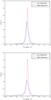 |
Fig. 7 Distribution of radial velocities P(Vr) of the solar siblings for the high and low dispersion cases. Top: the selection criteria of Eq. (1)is applied. Bottom: only the parallax in Eq. (1)is taken into account. The initial conditions of the Sun’s birth cluster here are Mc = 1125 M⊙ and Rc = 2pc, respectively. |
We computed the astrometric properties of the Sun’s siblings, such as parallaxes (ϖ), proper motions (μ), and radial velocities (Vr), for the cases of high and low dispersion. Given that for one simulation, the final distribution of solar siblings could be located all over the Galactic disk (e.g. top panel Fig. 6), we first need to select the stars that have the same galactocentric position as the Sun (R = 8.5 ± 0.5 kpc). The astrometric properties of the Sun’s siblings are then measured with respect to each of those Sun-like stars. We are interested in looking at the radial velocity of nearby solar siblings on almost the same orbit of the Sun. Therefore, following Brown et al. (2010) we choose the radial velocity of solar siblings that satisfy selection criteria given by Eq. (1). This equation makes use of the observationally established value of (VLSR + V⊙) /R⊙ in order to avoid introducing biases related to inadequacies in the simulated phase-space distribution of solar siblings (Brown et al. 2010).
However, since the proper motion of the recently discovered solar sibling – HD 162826 – does not correspond to the former selection criteria (see Ramírez et al. 2014), we also analyzed the radial velocities of solar siblings without taking their proper motion into account. The astrometric properties of the solar siblings were computed by using the Python’s package PyGaia5, which is a toolkit for basic Gaia data simulation, manipulation, and analysis.
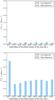 |
Fig. 8 Probability of finding solar siblings with radial velocity higher than 30 km s-1 in absolute value as a function of the initial mass of the Sun’s birth cluster. Top: the selection criteria of Eq. (1)is applied. Bottom: only the parallax in Eq. (1)is taken into account. |
In Fig. 7 we show the distribution of radial velocities P(Vr) of the solar siblings when Mc = 1125 M⊙ and Rc = 2pc. The velocity distribution was built by considering the Galactic parameters that produce either a high or low dispersion on the final distribution of the Sun’s siblings. As can be seen, P(Vr) is peaked at Vr ~ 0km s-1, and most of the radial velocities lie in the range −10 ≤ Vr ≤ 10km s-1, regardless of the selection criteria or the Galactic parameters. We found that there is a probability between 97% and 99% that the radial velocity of the Sun’s siblings lie in the previous range. The distribution shown in Fig. 7 is the same for the initial conditions of the Sun’s birth cluster listed in Table 8.
Since the star HIP 40317 has a radial velocity of 34 km s-1, we computed the probability of finding solar siblings with radial velocities higher than 30km s-1. The results are shown in Fig. 8. When the selection criteria of Eq. (1)is applied (see top panel of Fig. 8), such a probability is much less than 0.5%. However, if only the parallax in Eq. (1)is taken into account (see bottom panel of Fig. 8), the probability of finding solar siblings with high radial velocity could be up to ~2.5% for the current distribution of solar siblings highly dispersed on the Galactic disk (see blue bars). According to these results, it is unlikely to find solar siblings with Vr ~ 30km s-1.
Compared with solar neighbourhood observations, the estimated range of radial velocity is substantially less than the Galactic velocity dispersion (~45 km s-1) for stars with the solar age (see Holmberg et al. 2009). However, increased velocity dispersion could be explained as a natural consequence of the radial migration of solar age stars (Sellwood 2014) that come from many different birthplaces other than from the Sun’s.
On the other hand, it has also been shown that the giant molecular clouds (GMCs) could heat the disk stars and the orbits of stellar clusters (Gustafsson et al., in prep.), and they are missed in our models. Past studies have indicated that GMCs on their own are not able to heat the disk to the observed dispersion (Hänninen & Flynn 2002); however, a single star from star cluster might be greatly influenced. If we relax the 3 pc for the virial radius of the proto-cluster, the velocity dispersion in the cluster would be much larger than that of the chosen cluster half-mass radii, and the speed of the currently observable solar sibling can be explained easily. However, if we assumed that HD 162826 (Vr ~ 2km s-1) discovered by Ramírez et al. (2014) is a solar sibling, the primordial cluster should have had a smaller viral radius.
Thus, although we found that the abundance and age data favour sibling status for HIP 40317 (see Sect. 6), it is not directly supported by the dynamical arguments. We note that further studies of the dynamics of stars and stellar clusters in increasingly realistic conditions will continue to affect the studies of solar siblings.
8. Conclusions
We have obtained high-resolution spectra of 33 out of 57 solar sibling candidates, which were selected based on their colours and constraints in the proper motion and parallax space. Stellar parameters (Teff, log g, [Fe/H], vsini) were determined through both a purely spectroscopic approach and a partly physical method. Elemental abundances were determined by comparing observed spectra with synthetic spectra based on the stellar parameters obtained from our partly physical method (see Sect. 4.2.2). To calculate errors in elemental abundances, uncertainties of Teff, log g, and [Fe/H] were estimated to be about 40 K, 0.06 dex, and 0.03 dex based on five benchmark stars. Stellar ages were calculated from isochrones by maximizing the probability distribution functions.
Given the constraints on metallicity and stellar age, we found that four stars (HIP 10786, HIP 21158, HIP 40317, and HIP 51581) stand out from our candidate list. They have both metallicity and age close to the solar values within error bars. From an analysis of the Na, Mg, Al, Si, Ca, Ti, Cr, and Ni abundances of our observed candidates, we performed chemical tagging to identify cluster stars from the dissolved parent cluster. This resulted in a high probability that four sibling candidates (HIP 21158, HIP 24232, HIP 40317, and HIP 73600) share the same origin as the Sun. However, only HIP 40317 was identified as a possible solar sibling. We also noted that the rotational velocity of HIP 40317 could have the same rotational velocity as the Sun depending on the sini. We performed simulations of the Sun’s birth cluster in an analytical model of the Galaxy and found that most of the radial velocities of the solar siblings lie in the range −10 ≤ Vr ≤ 10km s-1, which is lower than the radial velocity of HIP 40317. We found that a fraction of stars from the star cluster might be accelerated to high velocity by heating sources; however, the probability of high radial velocity solar siblings based on our dynamical analysis is too low to prove that star HIP 40317 is a lost sibling of the Sun.
If we assume that HIP 40317 is a solar sibling, it means that only a very small fraction of sibling candidates (≲3%) are actually solar siblings. This is consistent with the prediction that within 100 pc from the Sun, about one to six are expected in our sample according to the simulations by Portegies Zwart (2009). More recently, Ramírez et al. (2014) have discovered only one solar sibling amongst 30 candidates, which is very similar to our results.
This leads to the question of how we can find solar siblings more efficiently. It is not clear what accuracy is needed to distinguish field stars and cluster stars. Since the probabilities of stars that are members of dissolved cluster are estimated based on an empirical function, a chemical tagging experiment on a large scale should calibrate against a number of known clusters (Mitschang et al. 2013). More chemical dimensions should be used to probe the formation sites of stars instead of nine elements. Furthermore, a simple Galactic potential was used to simulate the process of cluster disruption in both Portegies Zwart (2009) and Brown et al. (2010). It has been argued that solar siblings are unlikely to be found within the solar vicinity because of the influence of the perturbed Galactic gravitational field associated with spiral density waves (Mishurov & Acharova 2011). More detailed modelling of stellar orbits in a realistic potential could potentially prove more efficient at finding solar siblings.
IRAF is distributed by the National Optical Astronomy Observatory, which is operated by the Association of Universities for Research in Astronomy (AURA) under cooperative agreement with the National Science Fundation.
Acknowledgments
The authors wish to thank the referee, Ivan Ramírez, for thoughtful comments that improved the manuscript. We would like to thank Lennart Lindegren and Ross Church for valuable comments that improved the analysis and text of the paper. This project was completed under the GREAT – ITN network, which is funded through the European Union Seventh Framework Programme [FP7/2007-2013] under grant agreement no 264895. S.F. and G.R. are funded by grant No. 621-2011-5042 from The Swedish Research Council. T.B. is funded by grant No. 621-2009-3911 from The Swedish Research Council. This work also was supported by the Netherlands Research Council NWO (grants #643.200.503, #639.073.803, and #614.061.608) and by the Netherlands Research School for Astronomy (NOVA). This research made use of the SIMBAD database, operated at the CDS, Strasbourg, France.
References
- Adams, F. C. 2010, ARA&A, 48, 47 [NASA ADS] [CrossRef] [Google Scholar]
- Allen, C., & Santillan, A. 1991, Rev. Mex. Astron. Astrofis., 22, 255 [NASA ADS] [Google Scholar]
- Alonso, A., Arribas, S., & Martinez-Roger, C. 1995, A&A, 297, 197 [NASA ADS] [Google Scholar]
- Alonso, A., Arribas, S., & Martinez-Roger, C. 1996a, A&AS, 117, 227 [NASA ADS] [CrossRef] [EDP Sciences] [Google Scholar]
- Alonso, A., Arribas, S., & Martinez-Roger, C. 1996b, A&A, 313, 873 [NASA ADS] [Google Scholar]
- Antoja, T., Figueras, F., Romero-Gómez, M., et al. 2011, MNRAS, 418, 1423 [NASA ADS] [CrossRef] [Google Scholar]
- Aufdenberg, J. P., Ludwig, H.-G., & Kervella, P. 2005, ApJ, 633, 424 [NASA ADS] [CrossRef] [Google Scholar]
- Bagnulo, S., Jehin, E., Ledoux, C., et al. 2003, The Messenger, 114, 10 [NASA ADS] [Google Scholar]
- Batista, S. F. A., & Fernandes, J. 2012, New A, 17, 514 [Google Scholar]
- Batista, S. F. A., Adibekyan, V. Z., Sousa, S. G., et al. 2014, A&A, 564, A43 [NASA ADS] [CrossRef] [EDP Sciences] [Google Scholar]
- Bedell, M., Meléndez, J., Bean, J. L., et al. 2014, ApJ, 795, 23 [NASA ADS] [CrossRef] [Google Scholar]
- Bensby, T., Feltzing, S., & Lundström, I. 2003, A&A, 410, 527 [NASA ADS] [CrossRef] [EDP Sciences] [Google Scholar]
- Bensby, T., Adén, D., Meléndez, J., et al. 2011, A&A, 533, A134 [NASA ADS] [CrossRef] [EDP Sciences] [Google Scholar]
- Bensby, T., Feltzing, S., & Oey, M. S. 2014, A&A, 562, A71 [NASA ADS] [CrossRef] [EDP Sciences] [Google Scholar]
- Bertelli, G., Girardi, L., Marigo, P., & Nasi, E. 2008, A&A, 484, 815 [NASA ADS] [CrossRef] [EDP Sciences] [Google Scholar]
- Blackwell, D. E., & Lynas-Gray, A. E. 1998, A&AS, 129, 505 [NASA ADS] [CrossRef] [EDP Sciences] [Google Scholar]
- Bland-Hawthorn, J., Krumholz, M. R., & Freeman, K. 2010, ApJ, 713, 166 [NASA ADS] [CrossRef] [Google Scholar]
- Bobylev, V. V., Bajkova, A. T., Mylläri, A., & Valtonen, M. 2011, Astron. Lett., 37, 550 [NASA ADS] [CrossRef] [Google Scholar]
- Brown, A. G. A., Portegies Zwart, S. F., & Bean, J. 2010, MNRAS, 407, 458 [NASA ADS] [CrossRef] [Google Scholar]
- Bruntt, H., Bedding, T. R., Quirion, P.-O., et al. 2010, MNRAS, 405, 1907 [NASA ADS] [Google Scholar]
- Casagrande, L., Schönrich, R., Asplund, M., et al. 2011, A&A, 530, A138 [NASA ADS] [CrossRef] [EDP Sciences] [Google Scholar]
- da Silva, L., Girardi, L., Pasquini, L., et al. 2006, A&A, 458, 609 [NASA ADS] [CrossRef] [EDP Sciences] [Google Scholar]
- De Silva, G. M., Freeman, K. C., Asplund, M., et al. 2007a, AJ, 133, 1161 [NASA ADS] [CrossRef] [Google Scholar]
- De Silva, G. M., Freeman, K. C., Bland-Hawthorn, J., Asplund, M., & Bessell, M. S. 2007b, AJ, 133, 694 [NASA ADS] [CrossRef] [Google Scholar]
- De Silva, G. M., Freeman, K. C., & Bland-Hawthorn, J. 2009, PASA, 26, 11 [NASA ADS] [CrossRef] [Google Scholar]
- Dekker, H., D’Odorico, S., Kaufer, A., Delabre, B., & Kotzlowski, H. 2000, in SPIE Conf. Ser., 4008, eds. M. Iye, & A. F. Moorwood, 534 [Google Scholar]
- Demarque, P., Woo, J.-H., Kim, Y.-C., & Yi, S. K. 2004, ApJS, 155, 667 [NASA ADS] [CrossRef] [Google Scholar]
- Di Folco, E., Thévenin, F., Kervella, P., et al. 2004, A&A, 426, 601 [NASA ADS] [CrossRef] [EDP Sciences] [Google Scholar]
- Feltzing, S., Holmberg, J., & Hurley, J. R. 2001, A&A, 377, 911 [NASA ADS] [CrossRef] [EDP Sciences] [Google Scholar]
- Ferrers, N. M. 1877, Q. J. Pure Appl. Math., 14, 1 [Google Scholar]
- Flower, P. J. 1996, ApJ, 469, 355 [NASA ADS] [CrossRef] [Google Scholar]
- Frankowski, A., Jancart, S., & Jorissen, A. 2007, A&A, 464, 377 [NASA ADS] [CrossRef] [EDP Sciences] [Google Scholar]
- Freeman, K., & Bland-Hawthorn, J. 2002, ARA&A, 40, 487 [NASA ADS] [CrossRef] [Google Scholar]
- Gray, D. F., Tycner, C., & Brown, K. 2000, PASP, 112, 328 [NASA ADS] [CrossRef] [Google Scholar]
- Grevesse, N., Asplund, M., & Sauval, A. J. 2007, Space Sci. Rev., 130, 105 [Google Scholar]
- Gustafsson, B., Edvardsson, B., Eriksson, K., et al. 2008, A&A, 486, 951 [NASA ADS] [CrossRef] [EDP Sciences] [Google Scholar]
- Hänninen, J., & Flynn, C. 2002, MNRAS, 337, 731 [NASA ADS] [CrossRef] [Google Scholar]
- Holmberg, J., Nordström, B., & Andersen, J. 2009, A&A, 501, 941 [NASA ADS] [CrossRef] [EDP Sciences] [Google Scholar]
- Jofre, P., Heiter, U., Blanco-Cuaresma, S., & Soubiran, C. 2014a, Int. Workshop on Stellar Spectral Librairies, ASI Conf. Ser., 11, 159 [Google Scholar]
- Jofre, P., Heiter, U., Soubiran, C., et al. 2014b, A&A, 564, A133 [NASA ADS] [CrossRef] [EDP Sciences] [Google Scholar]
- Jørgensen, B. R., & Lindegren, L. 2005, A&A, 436, 127 [NASA ADS] [CrossRef] [EDP Sciences] [Google Scholar]
- Kaufer, A., Stahl, O., Tubbesing, S., et al. 1999, The Messenger, 95, 8 [Google Scholar]
- Kervella, P., Thévenin, F., Di Folco, E., & Ségransan, D. 2004, A&A, 426, 297 [NASA ADS] [CrossRef] [EDP Sciences] [Google Scholar]
- Kroupa, P. 2001, MNRAS, 322, 231 [NASA ADS] [CrossRef] [Google Scholar]
- Lada, C. J., & Lada, E. A. 2003, ARA&A, 41, 57 [NASA ADS] [CrossRef] [Google Scholar]
- Lallement, R., Welsh, B. Y., Vergely, J. L., Crifo, F., & Sfeir, D. 2003, A&A, 411, 447 [EDP Sciences] [Google Scholar]
- Mamajek, E. E., & Hillenbrand, L. A. 2008, ApJ, 687, 1264 [NASA ADS] [CrossRef] [Google Scholar]
- Martínez-Barbosa, C. A., Brown, A. G. A., & Portegies Zwart, S. 2015, MNRAS, 446, 823 [NASA ADS] [CrossRef] [Google Scholar]
- Mayor, M., Pepe, F., Queloz, D., et al. 2003, The Messenger, 114, 20 [NASA ADS] [Google Scholar]
- Mishurov, Y. N., & Acharova, I. A. 2011, MNRAS, 412, 1771 [NASA ADS] [CrossRef] [Google Scholar]
- Mitschang, A. W., De Silva, G., Sharma, S., & Zucker, D. B. 2013, MNRAS, 428, 2321 [NASA ADS] [CrossRef] [Google Scholar]
- Mitschang, A. W., De Silva, G., Zucker, D. B., et al. 2014, MNRAS, 438, 2753 [NASA ADS] [CrossRef] [Google Scholar]
- Nieva, M.-F., & Przybilla, N. 2012, A&A, 539, A143 [NASA ADS] [CrossRef] [EDP Sciences] [Google Scholar]
- Nissen, P. E., Chen, Y. Q., Carigi, L., Schuster, W. J., & Zhao, G. 2014, A&A, 568, A25 [NASA ADS] [CrossRef] [EDP Sciences] [Google Scholar]
- Nordström, B., Mayor, M., Andersen, J., et al. 2004, A&A, 418, 989 [NASA ADS] [CrossRef] [EDP Sciences] [Google Scholar]
- North, J. R., Davis, J., Bedding, T. R., et al. 2007, MNRAS, 380, L80 [NASA ADS] [CrossRef] [Google Scholar]
- Olsen, E. H. 1983, A&AS, 54, 55 [NASA ADS] [Google Scholar]
- Olsen, E. H. 1984, A&AS, 57, 443 [NASA ADS] [Google Scholar]
- Olsen, E. H. 1994, A&AS, 106, 257 [NASA ADS] [Google Scholar]
- Pancino, E., Carrera, R., Rossetti, E., & Gallart, C. 2010, A&A, 511, A56 [NASA ADS] [CrossRef] [EDP Sciences] [Google Scholar]
- Pavlenko, Y. V., Jenkins, J. S., Jones, H. R. A., Ivanyuk, O., & Pinfield, D. J. 2012, MNRAS, 422, 542 [NASA ADS] [CrossRef] [Google Scholar]
- Pelupessy, F. I., Jänes, J., & Portegies Zwart, S. 2012, New A, 17, 711 [Google Scholar]
- Perryman, M. A. C., Brown, A. G. A., Lebreton, Y., et al. 1998, A&A, 331, 81 [NASA ADS] [Google Scholar]
- Pichardo, B., Martos, M., & Moreno, E. 2004, ApJ, 609, 144 [NASA ADS] [CrossRef] [Google Scholar]
- Pichardo, B., Moreno, E., Allen, C., et al. 2012, AJ, 143, 73 [NASA ADS] [CrossRef] [Google Scholar]
- Plummer, H. C. 1911, MNRAS, 71, 460 [CrossRef] [Google Scholar]
- Portegies Zwart, S., McMillan, S. L. W., van Elteren, E., Pelupessy, I., & de Vries, N. 2013, Comp. Phys. Comm., 183, 456 [NASA ADS] [CrossRef] [Google Scholar]
- Portegies Zwart, S. F. 2009, ApJ, 696, L13 [NASA ADS] [CrossRef] [Google Scholar]
- Portegies Zwart, S. F., & Verbunt, F. 1996, A&A, 309, 179 [NASA ADS] [Google Scholar]
- Radick, R. R., Thompson, D. T., Lockwood, G. W., Duncan, D. K., & Baggett, W. E. 1987, ApJ, 321, 459 [NASA ADS] [CrossRef] [Google Scholar]
- Ramírez, I., Bajkova, A. T., Bobylev, V. V., et al. 2014, ApJ, 787, 154 [NASA ADS] [CrossRef] [Google Scholar]
- Reiners, A., & Schmitt, J. H. M. M. 2003, A&A, 398, 647 [NASA ADS] [CrossRef] [EDP Sciences] [Google Scholar]
- Romero-Gómez, M., Athanassoula, E., Antoja, T., & Figueras, F. 2011, MNRAS, 418, 1176 [NASA ADS] [CrossRef] [Google Scholar]
- Saar, S. H., & Osten, R. A. 1997, MNRAS, 284, 803 [NASA ADS] [CrossRef] [Google Scholar]
- Santos, N. C., Israelian, G., & Mayor, M. 2004, A&A, 415, 1153 [NASA ADS] [CrossRef] [EDP Sciences] [Google Scholar]
- Sellwood, J. A. 2014, Rev. Mod. Phys., 86, 1 [NASA ADS] [CrossRef] [Google Scholar]
- Sellwood, J. A., & Binney, J. J. 2002, MNRAS, 336, 785 [NASA ADS] [CrossRef] [Google Scholar]
- Soderblom, D. R. 2010, ARA&A, 48, 581 [NASA ADS] [CrossRef] [Google Scholar]
- Takeda, G., Ford, E. B., Sills, A., et al. 2007, ApJS, 168, 297 [NASA ADS] [CrossRef] [Google Scholar]
- Toonen, S., Nelemans, G., & Portegies Zwart, S. 2012, A&A, 546, A70 [NASA ADS] [CrossRef] [EDP Sciences] [Google Scholar]
- Torres, G. 2010, AJ, 140, 1158 [NASA ADS] [CrossRef] [Google Scholar]
- Valenti, J. A., & Fischer, D. A. 2005, ApJS, 159, 141 [NASA ADS] [CrossRef] [MathSciNet] [Google Scholar]
- Valenti, J. A., & Piskunov, N. 1996, A&AS, 118, 595 [NASA ADS] [CrossRef] [EDP Sciences] [Google Scholar]
- van Leeuwen, F. 2007, A&A, 474, 653 [NASA ADS] [CrossRef] [EDP Sciences] [Google Scholar]
- Volz, U., Majerus, M., Liebel, H., Schmitt, A., & Schmoranzer, H. 1996, Phys. Rev. Lett., 76, 2862 [NASA ADS] [CrossRef] [PubMed] [Google Scholar]
- Wielen, R., Fuchs, B., & Dettbarn, C. 1996, A&A, 314, 438 [NASA ADS] [Google Scholar]
- Yi, S. K., Kim, Y.-C., & Demarque, P. 2003, ApJS, 144, 259 [NASA ADS] [CrossRef] [Google Scholar]
All Tables
Stellar parameters for the Sun and four benchmark stars used to develop our methodology.
Errors in the abundances due to the uncertainties in stellar parameters: Teff ± 40 K, log g ± 0.06 dex, [Fe/H] ± 0.03 dex.
All Figures
|
Fig. 1 Colour–magnitude diagram showing the absolute magnitude MV versus. B − V. The contour plot shows the distribution of the stars in the Hipparcos catalogue with σϖ/ϖ ≤ 0.1 and σB − V ≤ 0.05 (van Leeuwen 2007). The spectra of the 33 sibling candidates are indicated with triangles. The solid line shows an isochrone with the age (5 Gyr) and metallicity of the Sun (Demarque et al. 2004). The vertical dashed line indicates our cut-off at B − V = 0.4. |
| In the text | |
|
Fig. 2 a) HR diagram for the sample when a)log g is based on Fe i-Fe ii ionization equilibrium and b) when log g is based on Hipparcos parallaxes. Four isochrones at solar metallicity and four different ages (1, 3, 5, and 6 Gyr) according to the Yonsei-Yale models (Demarque et al. 2004) are also shown. |
| In the text | |
|
Fig. 3 a)Teff,r − Teff,p vs. Teff,p, where Teff,r represents the recommended effective temperature. Teff,p is the best-determined effective temperature from our methodology. Five symbols stand for the five benchmark stars, while two (or three) of the same symbol indicates that spectra obtained with different instruments were analysed. It is the same for the log gr and log gp that are shown in panel b). |
| In the text | |
|
Fig. 4 Sensitivity of [Fe/H] to changes in stellar parameters for the Sun. A significant correlation between Δ[Fe/H] and ΔTeff exists, while the trend between Δ[Fe/H] and Δlog g is hardly detected. |
| In the text | |
|
Fig. 5 Elemental abundance ratios [X/Fe] relative to Fe. Dashed lines indicate solar values. |
| In the text | |
|
Fig. 6 Final distribution on the Galactic plane of solar siblings when Mc = 804.6 M⊙ and Rc = 3 pc. The final phase-space coordinates of the solar siblings depend on the configuration of the Galactic potential. Top: the Sun’s siblings are dispersed on the Galactic disk. Bottom: the solar siblings are located in a specific region on the Galactic disk. The dashed black lines represent the potential of the spiral arms at the end of the simulation. |
| In the text | |
|
Fig. 7 Distribution of radial velocities P(Vr) of the solar siblings for the high and low dispersion cases. Top: the selection criteria of Eq. (1)is applied. Bottom: only the parallax in Eq. (1)is taken into account. The initial conditions of the Sun’s birth cluster here are Mc = 1125 M⊙ and Rc = 2pc, respectively. |
| In the text | |
|
Fig. 8 Probability of finding solar siblings with radial velocity higher than 30 km s-1 in absolute value as a function of the initial mass of the Sun’s birth cluster. Top: the selection criteria of Eq. (1)is applied. Bottom: only the parallax in Eq. (1)is taken into account. |
| In the text | |
Current usage metrics show cumulative count of Article Views (full-text article views including HTML views, PDF and ePub downloads, according to the available data) and Abstracts Views on Vision4Press platform.
Data correspond to usage on the plateform after 2015. The current usage metrics is available 48-96 hours after online publication and is updated daily on week days.
Initial download of the metrics may take a while.