| Issue |
A&A
Volume 575, March 2015
|
|
|---|---|---|
| Article Number | A89 | |
| Number of page(s) | 9 | |
| Section | Stellar atmospheres | |
| DOI | https://doi.org/10.1051/0004-6361/201424844 | |
| Published online | 02 March 2015 | |
Center-to-limb polarization in continuum spectra of F, G, K stars⋆
1
Kiepenheuer-Institut für Sonnenphysik (KIS),
Schöneckstrasse 6,
79104
Freiburg,
Germany
e-mail: kostogryz@kis.uni-freiburg.de; sveta@kis.uni-freiburg.de
2
Main Astronomical Observatory of NAS of Ukraine,
Zabolotnoho str. 27,
03680
Kyiv,
Ukraine
3
NASA Astrobiology Institute, Institute for Astronomy, University
of Hawaii, Honolulu,
HI
96822,
USA
Received: 21 August 2014
Accepted: 23 December 2014
Context. Scattering and absorption processes in stellar atmosphere affect the center-to-limb variations of the intensity (CLVI) and the linear polarization (CLVP) of stellar radiation.
Aims. There are several theoretical and observational studies of CLVI using different stellar models, however, most studies of CLVP have concentrated on the solar atmosphere and have not considered the CLVP in cooler non-gray stellar atmospheres at all. In this paper, we present a theoretical study of the CLV of the intensity and the linear polarization in continuum spectra of different spectral type stars.
Methods. We solve the radiative transfer equations for polarized light iteratively assuming no magnetic field and considering a plane-parallel model atmospheres and various opacities.
Results. We calculate the CLVI and the CLVP for Phoenix stellar model atmospheres for the range of effective temperatures (4500 K–6900 K), gravities (log g = 3.0−5.0), and wavelengths (4000–7000 Å), which are tabulated and available at the CDS. In addition, we present several tests of our code and compare our results with measurements and calculations of CLVI and the CLVP for the Sun. The resulting CLVI are fitted with polynomials and their coefficients are presented in this paper.
Conclusions. For the stellar model atmospheres with lower gravity and effective temperature the CLVP is larger.
Key words: polarization / radiative transfer / scattering / stars: atmospheres / methods: numerical
Full Tables 1 and 2, and coefficients of polynomials are only available at the CDS via anonymous ftp to cdsarc.u-strasbg.fr (130.79.128.5) or via http://cdsarc.u-strasbg.fr/viz-bin/qcat?J/A+A/575/A89
© ESO, 2015
1. Introduction
Stellar intrinsic polarization from scattering is an important effect for investigating the physical and geometrical properties of stars and stellar environments. The first theoretical prediction of linear polarization of continuous light in the emergent radiation from the early-type stars was made by Chandrasekhar (1946). He solved the radiative transfer equation for a purely scattering atmosphere in radiative equilibrium and showed that polarization from the light scattered at the limb of the stellar disk is considerable, ~12%, and could be detected under favourable conditions. Later, Rucinski (1970) showed that the high value of limb polarization predicted by Chandrasekhar could be only considered as the upper limit for early-type stars, while polarization for cooler stars would be much smaller. Harrington & Collins (1968) demonstrated that rotation distortion (early-type stars are usually fast rotators) and limb darkening affect the symmetry of early-type stars and should produce detectable polarization under suitable conditions and geometry. However, Thomson scattering is the main source of scattering opacity in the early spectral type stars, but not for the solar or the late-type stars (see, Clarke, 2010).
The best representative candidate of the solar-type stars is our Sun. As the polarized spectrum formed by coherent scattering is a rich source of information about the atmosphere, the scientific community has paid a lot of attention to studying the polarized spectrum of the Sun (e.g. Fluri & Stenflo, 1999; Berdyugina et al., 2002; Stenflo, 2005; Trujillo Bueno & Shchukina, 2009, and many others). This spectrum was called the Second Solar Spectrum (Ivanov, 1991; Stenflo & Keller, 1997). It is characterized by a polarized continuous background on which a rich variety of both intrinsically polarized and depolarized lines are superimposed. Polarized lines look like “emission” and depolarized lines look similar to “absorption” lines with respect to continuum polarization. However, many lines are also weakly polarized or depolarized by magnetic fields due to the Hanle effect. The polarization in the lines and the continuum are usually on the same order of magnitude, and a common zero level should be used as the reference for the line polarization. There are several observational studies of center-to-limb variation of linear polarization in different spectral lines and adjacent continua for the Sun (Leroy, 1972; Mickey & Orrall, 1974; Wiehr, 1975; Wiehr & Bianda, 2003; Stenflo, 2005). The maximum continuum polarization on the Sun is up to 1.7% at the limb for wavelength 3000Å (Stenflo, 2005). Wiehr & Bianda (2003) measured the CLVP in continuum of 0.12% in two wavelength intervals (3Å) overlapping each other near 4506 Å where no significant line polarization occurs. These measurements are very difficult since the continuum limb polarization is superposed with strong intensity gradient at the limb, and the absolute value of polarization is hard to measure. Knowing the degree of polarization in the continuum from theoretical predictions helps to interpret the observations.
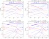 |
Fig. 1 Normalized scattering (dashed lines) and absorption (solid lines) coefficients as a function of optical depth. Titles on each of the panels describe the model parameters for calculation of the opacities. Solid lines show all important absorption opacities and dashed lines represent all scattering opacities. Thick solid and thick dashed lines are the normalized total absorption and total scattering opacities, respectively. |
As the solar disk can be resolved, it is possible to detect the limb polarization (Gandorfer, 2000, 2002, 2005) and the center-to-limb variation of polarized light (Leroy, 1972; Mickey & Orrall, 1974; Wiehr, 1975; Wiehr & Bianda, 2003) directly. In most cases, however, it is not possible to resolve a stellar disk to measure the CLVP of its radiation. It is expected that any intrinsic polarization of solar-type stars integrated over the disk is likely to be very small, and it can only be increased if the symmetry of the disk is broken. This is the case if a star possesses a nonspherical radiation field as a result of geometric distortion, for example, due to fast rotation or tides in binaries, or if it has a nonuniform photospheric surface brightness. For example, the latter can happen in the case of starspots or inhomogeneities in the outer atmosphere where scattering takes place, or because of a transiting exoplanet that blocks a part of the stellar radiation and, hence, breaks the symmetry of the stellar disk.
Carciofi & Magalhães (2005), Kostogryz et al. (2011a,b), and Frantseva et al. (2012) attempted to estimate the polarization signal of a star due to the symmetry breaking effect that appears when a planet transits the stellar disk. They showed that the polarization degree of the transiting exoplanetary system is very sensitive to the intrinsic center-to-limb polarization of the host star, however, they used simplified approximations for the stellar limb polarization. In this paper, we present a more realistic theoretical calculation of polarized light in stellar atmospheres by solving the radiative transfer equation for the visible spectra of F, G, and K stars. In Sect. 2 we focus on the theoretical approach to our calculations and on the opacities in the stellar model atmosphere. Section 3 presents the results of our calculations of CLVI and CLVP for different stellar model atmospheres. In addition, we present several tests of our computer code. Finally, we summarize our findings in Sect. 4.
2. Theoretical approach to continuum polarization calculations
2.1. Stellar models and opacities.
Models of stellar atmospheres are the most important input in our calculations. In our simulations we used Phoenix local thermodynamic equilibrium (LTE) models (Hauschildt et al., 1999) for the range of the effective temperatures from 4500 K to 6900 K and the surface gravity log g from 3.0 to 5.0. In addition to the Phoenix models, we employed several semiempirical solar model atmospheres of the quiet Sun, such as FALC (averaged quiet Sun), FALA (the supergranular cell center), FALP (the plage model; Fontenla et al. 1993) and HSRA (averaged quiet Sun; Gingerich et al. 1971).
We calculated the opacities for different wavelengths using the code SLOC (Berdyugina, 1991) for stars of different spectral types, assuming solar abundances and metallicity. For the calculation of the stellar continuum opacities we have taken the following contributors into account:
-
Scattering opacity: Thomson scattering on free electrons e− and Rayleigh scattering on HI, HeI, H2, CO, H2O, and other molecules.
-
Absorption opacity: free-free (ff) and bound-free (bf) transitions in H−, HI, HeI, He−,
 ,
,  , and metal photoionization.
Figure 1 shows the main contributions to the stellar continuum opacities (scattering and absorption coefficients normalized to the total opacity) for the different stellar atmosphere models with different effective temperatures, gravities, and for wavelengths of 4000 Å and 6000 Å. The optical depth scale corresponds to the total opacity at a given wavelength.
As expected, the most important opacity source in the visible wavelengths in the atmospheres of F, G, K stars is absorption by the negative ion hydrogen H−. Another absorption opacity source that plays an important role in the deeper layers of stellar atmospheres is , which is a proton-hydrogen atom encounter. In addition, in deeper layers of the solar atmosphere HI absorption is more noticeable than in cooler atmospheres, especially at longer wavelengths. These opacities act as pure absorption and do not produce any polarization.
The main contribution to the polarization of the stellar continuum spectrum are Rayleigh scattering on neutral hydrogen HI (Chandrasekhar, 1960), whish is dominated by scattering in the distant line wings of the Lyman series lines (Stenflo, 2005) and Rayleigh scattering by molecular hydrogen H2, which becomes considerable in cooler stellar atmospheres. Thomson scattering on free electrons is still an important source of opacity for the Sun, whereas it is completely negligible for cooler stars.
It is also important to note that for the stellar model atmospheres with an effective temperature of 4500 K and log g = 4.5 at wavelength of 4000 Å (Fig. 1c, cooler atmosphere at shorter wavelength) scattering becomes larger than absorption deeper in the atmosphere at τ ≈ 3 × 10⁻⁴, as compared with the solar atmosphere model where it occurs at τ ≈ 1 × 10⁻⁵ (Fig. 1a). This relative increase of scattering opacity in the stellar atmosphere leads to an absolute increase of the linear polarization in cool atmospheres.
2.2. Numerical solution of the radiative transfer problem
We have implemented a numerical solution of the radiative transfer problem for polarized light in the solar continuum as described in Fluri & Stenflo (1999). We have developed our code ContPol based on this description and applied it to the stellar continuum spectra. Hereafter, we briefly present the formulation of the transfer problem for polarized light. For this, we consider a plane-parallel, static atmosphere with homogeneous layers and without magnetic fields. The anisotropy that is necessary for scattering polarization is caused by the center-to-limb variation of the intensity, i.e., temperature gradient within the atmosphere.
Normally, polarized radiation is described by four Stokes parameters I,Q,U, and V. In our calculations, we choose the coordinate system in such a way that Stokes Q represents the linear polarization in the direction parallel to the stellar limb, and this means that Stokes U is equal to zero. Stokes V is equal to zero because Rayleigh scattering does not produce circular polarization and we neglect magnetic field effects. So the Stokes vector is defined as follows:  (1)The polarized radiative transfer equation in the absence of magnetic fields is written as
  (2)where μ = cosθ defines a line of sight direction with respect to the plane of the atmosphere. The parameters Sν and Iν depend on τ and μ.
Here, dτν is the optical depth defined as  (3)where kc is the continuum absorption coefficient, σc is the continuum scattering coefficient and z is the geometric height.
The total source function Sν is given by  (4)where Bν describes pure absorption and is determined by the Planck function as follows
  (5)and Ss,ν expresses the contribution from all radiative sources associated with scattering. It can be written as
  (6)where μ′ is the direction of the incident radiation within the differential solid angle dΩ′. PR is the Rayleigh phase matrix that takes the angular dependence of Rayleigh and Thomson scattering into account and is given by Stenflo (1994).
As in the case of Fluri & Stenflo (1999), we first calculate the scattering and absorption coefficients, as described in Sect. 2.1 while neglecting polarization. Then the radiative transfer problem for polarized light is solved with previously computed kc and σc. To obtain a numerical solution of the radiative transfer equations we employ the Feautrier method. This method for nonpolarized radiation is discussed by Mihalas (1978), while we extend it to solve the radiative transfer equations for polarized light.
We use the following boundary conditions: the diffusion approximation by Mihalas (1978) for Stokes I is assumed at the bottom of the stellar atmosphere, while at the top of the atmosphere there is no incoming radiation, i.e., I = 0. For both boundary conditions we assume no polarization, so the Stokes parameter Q = 0. We make several iterations to achieve convergence at each level of the atmosphere. Usually more iterations are needed for atmospheres with large scattering contributions.
3. Results
3.1. Purely scattering atmosphere
The classical solution of the radiative transfer equation for an ideal, purely scattering plane-parallel atmosphere shows the increase of the polarization amplitude up to 11.7% at the very limb of a stellar disk (Chandrasekhar, 1960). Pure scattering atmosphere means that the total opacity is due to scattering and no absorption occurs. Following Fluri & Stenflo (1999), we obtain the pure scattering atmosphere solution by artificially redefining the scattering coefficient as the sum of kc and σc and setting the absorption coefficient to zero. After such assumptions, the Stokes I/Icenter and Q/I components of the outgoing continuum radiation field turn out to be independent of frequency and of all thermodynamic properties, so basically any initial atmosphere can be used for this test.
As was shown in Fluri & Stenflo (1999) all solar model atmospheres give identical center-to-limb variations of the polarization and intensity for all wavelengths considered, from 4000 Å to 8000 Å. With our code we tested different solar atmosphere models (FALC, HSRA) and Phoenix atmosphere models with effective temperatures 5800 K, 4000 K and log g = 4.5 for the 4000 Å to 8000 Å wavelength range. As is shown in Fig. 2, we can reproduce precisely Chandrasekhar’s solution for pure scattering atmosphere for all considered models. This proves that scattering has been correctly calculated in the code.
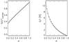 |
Fig. 2 CLVI (left panel) and CLVP (right panel) for the exact solution (crosses) given by Chandrasekhar (1960) and our calculation of the radiative transfer equation for polarised light for pure scattering atmosphere (solid line). The same solid line is obtained for all wavelengths from 4000 Å to 8000 Å and for different solar and stellar atmospheres assuming pure scattering as described in the text. |
3.2. Limb darkening
The solar limb darkening was measured many times by different observers who fitted the observed center-to-limb variations of the intensity with suitable analytical functions or limb darkening laws, usually employing up to five free parameters that in general depend mostly on wavelength.
To compare our calculations with the observed solar CLVI, we have chosen the analytical polynomial function P5(μ) given by Neckel & Labs (1994) who fitted them to mean continuum measurements, corrected for scattered light. Any new measurements may differ somewhat from this analytical function because of the temporal variability of the limb darkening caused by surface features (e.g., plages).
Figure 3 presents observed and calculated solar limb darkening for three different wavelengths. As is seen for λ = 4000 Å we have very good agreement, while for wavelength of 5000 Å and 6000 Å we have small discrepancies. Considering natural variations of the solar limb darkening around the Neckel & Labs (1994) limb darkening polynomial function, we can conclude that limb darkening for the Sun is well reproduced by our calculations.
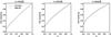 |
Fig. 3 Solar CLVI for different wavelengths. Solid lines in all panels depict our modeled continuum polarization (ContPol) for the HSRA model atmosphere and dashed lines show observations obtained by Neckel & Labs (1994). |
Likewise, we compared our single wavelength continuum calculations for Phoenix stellar models with the results by Claret et al. (2013) for broadband filters U, B, V. These filters include contributions from hundreds of angstroms with many spectral lines, especially for cooler atmospheres. As expected for hot stars (>5800 K) we can reproduce well broadband simulations since there are not so many lines and continuum dominates. With decreasing effective temperatures of the stellar models we have larger discrepancies. For cooler atmospheres there are more spectral lines that contributed to CLVI, therefore the disagreement between our calculations is larger there. Naturally, to explain broadband observations of the center-to-limb variations we need to take all the spectral lines contributing to the bandpass of the filter into account, while our present calculations are useful for explaining the monochromatic measurements at the continuum level.
3.3. Solar limb polarization
We calculate continuum polarization for different solar model atmospheres (FALA, FALC, FALP, HSRA, and Phoenix) and for various wavelengths (4000 Å, 5000 Å and 6000 Å). We show that the CLVP depends on the model (Fig. 5), and this is in a good agreement with Fluri & Stenflo (1999). The difference in polarization at the limb μ = 0.1 between FALA (the supergranular cell center) and FALP (plage) models is the largest for all considered wavelengths. For example, for wavelength 4000 Å for FALA Q/I(μ = 0.1) = 0.36%, while for FALP Q/I(μ = 0.1) = 0.24%, which is more than 30% different. Other wavelengths exhibit similar behavior. Apart from our calculations, we also show in Fig. 5 the center-to-limb variation of the continuum linear polarization described by the analytical approximations taken from Fluri & Stenflo (1999, thick dashed line) and from Stenflo (2005, thick dotted line). To calculate the continuum polarization with the empirical equations from both Fluri & Stenflo (1999) and Stenflo (2005), one needs the solar limb darkening, which they have not given in their papers. To compare with these two approximations, we use the limb darkening from our simulation for the FALC model in both cases. To reproduce the Fluri & Stenflo (1999) approximation, which depends on the model, we choose all parameters for the FALC model from their paper.
To understand the continuum polarization variations for different solar atmosphere models, we analyze the opacities for all models presented in Fig. 4. Since the only contributor to linear polarization calculations is scattering, the optical depth in the atmosphere where scattering becomes dominant determines the amount of observable linear polarization. As is seen in Fig. 4, this depth varies for different solar models. For example, the lowest CLVP (Fig. 5) occurs for the Phoenix and FALP models. For the Phoenix model the scattering opacity only dominates at the very top of the atmosphere, where the number of scattering particles is smaller. However, for both of these models absorption is still high in the upper levels of the atmosphere, which reduces radiation that can be scattered. For the other models the absorption decreases rapidly toward the top of the atmosphere and the CLVP is somewhat higher. Opacities variations are due to different temperature profiles in these models.
The only way to choose the suitable model is to compare modeled continuum polarization with observations. Stenflo (2005) derived empirical values of continuum polarization on the Sun, which were extracted from the Second Solar Spectra (Gandorfer, 2000, 2002, 2005) with the help of a one-parameter model for behavior of depolarizing lines. He assumed that polarization degrees in the cores of the deepest depolarizing lines equal to zero, which, however, may not be fulfilled in blue region. Stenflo (2005) found that his inferred continuum polarization is lower than that predicted by Fluri & Stenflo (1999), however, the difference is within the range of the empirical values. At 4500 Å the lower and upper limit of polarization at the limb are ~0.07% and ~0.12% (Stenflo, 2005), respectively. Wiehr & Bianda (2003) observed the center-to-limb variation of the scattering polarization in a narrow continuum window at 4506−4508 Å up to the extreme solar limb. They measured the polarization of ~0.12% at disk position μ = 0.1. This is in a very good agreement with Stenflo (2005). We believe that the upper limit is more realistic according to the chosen procedure, which is described in Stenflo (2005). Wiehr & Bianda (2003) also showed that the calculations by Fluri & Stenflo (1999) for the model FALC fit very well the observations up to the limb distance of μ = 0.025, but at exactly μ = 0.1 the measurements have a small discrepancy from the model and this deviation is within the noise level. Modeling scattering polarization in spectral lines also showed that FALA, FALC, and FALP models lack necessary anisotropy (Bommier et al., 2006; Shapiro et al., 2011; Kleint et al., 2011).
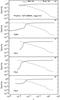 |
Fig. 4 Normalized scattering (dashed) and absorption (solid) coefficients as a function of optical depth for different solar model atmospheres at 4000 Å wavelength. Different panels correspond to different solar model atmospheres: a) Phoenix model with effective temperature of 5800 K and log g of 4.5; b) HSRA; c) FALC; d) FALA; e) FALP. |
In Fig. 6 we compare solar disk polarization measurements from the literature (symbols) with our modeling for the FALC, FALA, FALP, and HSRA model atmospheres (different line styles). All of the data were not obtained in the solar continuum, which can lead to a disagreement between observations and calculations caused by line polarization contamination. In Fig. 6a, polarimetric observations made by Leroy (1972) in the wing of the Fe I line are presented. They are systematically higher at all limb angles (but are within the error bars for smaller angles) than the calculated continuum polarization for all solar model atmospheres. This is probably because of the Fe I line contribution as well as numerous polarized CN violet system lines in this region (Shapiro et al., 2011). A similar situation occurs in Fig. 6b, where measurements by Wiehr (1975) are presented. In this case we see the largest discrepancy between measurements and calculations. However, this discrepany can be explained by a contribution from the nearby strong Ca I line at λ = 4227 Å blended with Fe I and Fe II lines. The Ca I line has broad wings with a large polarization (Gandorfer, 2002), and the adjacent continuum at 4235 Å is apparently contaminated by the line wing. The most recent polarization measurements in the solar continuum (λ = 4506 Å) obtained by Wiehr & Bianda (2003) are presented in Fig. 6c. These data show the best agreement with the solar models, except perhaps that shown with the dotted line (FALP model). The data in Fig. 6d were obtained at λ = 4876 Å. According to the second solar spectrum atlas (Gandorfer, 2000), at this wavelength there is a slightly depolarizing Fe I line with Q/I of 0.01% lower than the nearby continuum. Therefore, we can expect a somewhat higher polarization in the continuum leading to a better agreement with the solar models. The next four panels (e, f, g, and h) present the data obtained at longer wavelengths where the polarization is smaller and is more difficult to measure. However, despite small disagreements caused by either line contributions or large measurement errors, it appears that our computations for solar models reproduce well the available polarimetric measurements in the continuum made by different authors in different years. It is definitely worth investigating this subject in more detail and obtain more precise measurements at several wavelengths and limb angles, but this is outside the scope of this paper.
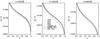 |
Fig. 5 Center-to-limb variation of linear polarization. Different kind of lines depict our calculations for different model atmospheres: FALC, FALP, FALA, HSRA, and LTE5800-45 (Phoenix model for Teff = 5800 K and log g = 4.5). The thick dashed line (F&S99, FALC) corresponds to the analytical function for the FALC model taken from Fluri & Stenflo (1999), while the thick dotted line (S05, FALC) represents the analytical function taken from Stenflo (2005). |
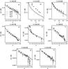 |
Fig. 6 A comparison of modeled and observed center-to-limb variation of linear polarization. Different kind of lines depict our calculations for different model atmospheres: FALC, FALP, FALA, HSRA labeled in plot a). Symbols in a), d), f), g), h) show the solar disk polarization measured by Leroy (1972), in c) by Wiehr & Bianda (2003), in b) by Wiehr (1975), and in e) by Mickey & Orrall (1974). The wavelength at which the measurement was taken is given in each plot individually. |
Calculated center-to-limb variation of intensity for different stellar parameters. All values of I(μ) /I(1.0) = 1.0 at μ = 1.0.
Calculated center-to-limb variation of linear polarization in continuum spectra of different stars. All values of Q/I(μ) = 0.0 at μ = 1.0.
3.4. Stellar limb polarization
In contrast to numerous investigations of the solar continuum polarization, the limb polarization of other stars has not been systematically studied as much. Harrington (1970) presented the first calculations of stellar center-to-limb variation of linear polarization in the case of gray plane-parallel atmosphere. In this paper we present our calculations of the center-to-limb variation of the linear polarization in continuum for a large range of stellar models for F, G, K stars in the case of non-gray atmosphere.
We calculate the radiative transfer equations for the grid of Phoenix model atmospheres within the range of effective temperatures from 4500 K to 6900 K at steps of 100 K and for log g from 3.0 to 5.0 at steps of 0.5. For different wavelengths, effective temperatures, log g and various position on the stellar disk μ, we present the value of CLVI in Table 1 and CLVP in Table 2.
In addition, we fit each CLVI with a polynomial and also present the table of the polynomial coefficients. The polynomials used are the following:  (7)where f(μ) is the CLVI (I(μ) /I(1.0)). Note that for a good fit to the CLVI, a fourth order polynomial is required. The coefficients of polynomials are only available in electronic form at the CDS.
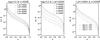 |
Fig. 7 Center-to-limb variation of the continuum polarization for different stellar models. The title above each of the panels indicates the fixed parameters, while labels on each plot describe different curves. Note continuum polarisations are given in logarithmic scale. |
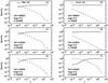 |
Fig. 8 Normalized scattering and absorption coefficients as a function of optical depth τ for Phoenix stellar model atmospheres. Different panels show the opacities for various parameters of the models that are described in a legend of each panels. Panels a) and b) present the opacities for stars with effective temperature of 5800 K and log g of 4.5 for different wavelengths of 4000 Å and 7000 Å, respectively. Panels c) and d) are for stars with the same log g and at the same wavelengths, respectively but for effective temperature of 5300 K. Panels e) and f) are for stars with identical effective temperature of 4500 K and at the same wavelength of 4000 Å except for two different values log g of 4.5 and 3.0, respectively. |
In Fig. 7 we show the dependence of stellar continuum polarization on the model effective temperature, gravity, and wavelength. As seen in Fig. 7 (first panel) the cooler the star, the higher the continuum polarization. As the dominant scattering opacity is due to Rayleigh scattering, higher polarization for shorter wavelengths is obtained (see Fig. 7, second panel). The last panel in Fig. 7 shows that larger gravity of a star leads to lower linear polarization. Therefore, the largest continuum polarization can be detected on low-gravity cool stars. As in the case of the Sect. 3.3, we analyze the normalized absorption and scattering opacities to explain the continuum polarization behavior for different stars. Figure 8 presents opacity calculations for three effective temperatures, two log g values and two different wavelengths. As mentioned above, one of the important factors for the continuum polarization calculation is the optical depth in the atmosphere where scattering processes dominate over absorption. Hence, Fig. 8a, c, e shows that for the same log g and wavelength region, scattering starts to dominate deeper in the atmosphere for cooler stars than for solar-type stars, which leads to increasing linear polarization in cool stars (Fig. 7, first panel). We also note that for a given wavelength and a given temperature scattering becomes dominant at a deeper atmospheric level for stars with a gravity of log g = 3.0 compared to stars with log g = 4.5 (Fig. 8e, f). For the red part of the visual spectrum 7000 Å (Fig. 8b), where Rayleigh scattering is not so strong, the absorption is the dominant opacity over the entire atmosphere, and that leads to decreasing linear polarization.
4. Summary
We have solved the radiative transfer equations for polarized light in the continuum spectra accounting for absorption, Rayleigh, and Thomson scattering. Thomson scattering is more important for hotter stellar atmospheres, while for almost all stellar atmospheres considered here the most important opacities are Rayleigh scattering on neutral hydrogen and absorption by a negative hydrogen ion. For cooler atmospheres, Rayleigh scattering on molecular hydrogen becomes more prominent but is still not dominating in the considered range of the effective temperatures of a star.
We present the results of our calculations of the CLVI and CLVP in the stellar continuum spectra with effective temperatures 4500 K–6900 K and gravities log g = 3.0−5.0 and in the spectral range from 4000 Å to 7000 Å. Since Rayleigh scattering is dominant, the scattering polarization is larger in the blue wavelengths.
The deeper in the atmosphere the scattering opacity becomes dominant over the absorption opacity, the larger the linear polarization can be observed. Since in low-gravity cool stars scattering becomes dominant very deep in the atmosphere, the CLVP is larger for cool giants. So, low gravity cool stars have much larger polarization in their continuum spectra although they have smaller CLV of the intensity.
We conclude that linear polarization is a sensitive tool to test stellar model atmospheres, with respect to their temperature profiles and particle density distribution. In addition, for testing the stellar models, the CLVP is very useful for calculations of stellar disk symmetry breaking effects, such as planetary transits and presence of spots on the stellar disk, which we will present in a forthcoming paper.
Acknowledgments
This work was supported by the European Research Council Advanced Grant HotMol(ERC-2011-AdG291659). We thank Martin Kürster for the comments and suggestions and an anonymous referee for comments that improved this paper.
References
- Berdyugina, S. V. 1991, Bull. Crimean Astrophysical Observatory, 83, 89 [Google Scholar]
- Berdyugina, S. V., Stenflo, J., & Gandorfer, A. 2002, A&A, 388, 1062 [NASA ADS] [CrossRef] [EDP Sciences] [Google Scholar]
- Bommier, V., Landi Degl’ Innocenti, E., Feautrier, N., & Molodij, G. 2006, A&A, 458, 625 [NASA ADS] [CrossRef] [EDP Sciences] [Google Scholar]
- Carciofi, A. C., & Magalhães, A. M. 2005, ApJ, 635, 570 [NASA ADS] [CrossRef] [Google Scholar]
- Chandrasekhar, S. 1946, ApJ, 103, 351 [NASA ADS] [CrossRef] [Google Scholar]
- Chandrasekhar, S. 1960, Radiative Transfer (New York: Dover) [Google Scholar]
- Claret, A., Hauschildt, P. H., & Witte, S. 2013, A&A, 552, A16 [NASA ADS] [CrossRef] [EDP Sciences] [Google Scholar]
- Clarke, D. 2010, Stellar Polarimetry (Weinheim: Wiley-VCH Verlag GmbH and Co. KGaA) [Google Scholar]
- Fluri, D. M., & Stenflo, J. O. 1999, A&A, 341, 902 [NASA ADS] [Google Scholar]
- Fontenla, J. M., Avrett, E. H., & Loeser, R. 1993, ApJ, 406, 319 [NASA ADS] [CrossRef] [Google Scholar]
- Frantseva, K., Kostogryz, N. M., & Yakobchuk, T. M. 2012, Adv. Astron. Space Phys. 2, 146 [Google Scholar]
- Gandorfer, A. 2000, The Second Solar Spectrum: A high spectral resolution polarimetric survey of scattering polarization at the solar limb in graphical representation. Volume I: 4625 Å to 6995 Å (Zürich: vdf Hochschulverlag) [Google Scholar]
- Gandorfer, A. 2002, The Second Solar Spectrum: A high spectral resolution polarimetric survey of scattering polarization at the solar limb in graphical representation. Volume II: 3910 Å to 4630 Å (Zürich: vdf Hochschulverlag) [Google Scholar]
- Gandorfer, A. 2005, The Second Solar Spectrum: A high spectral resolution polarimetric survey of scattering polarization at the solar limb in graphical representation. Volume III: 3160 Å to 3915 Å (Zürich: vdf Hochschulverlag) [Google Scholar]
- Gingerich, O., Noyes, R. W., Kalkofen, W., et al. 1971, Sol. Phys., 18, 347 [NASA ADS] [CrossRef] [Google Scholar]
- Harrington, J. P. 1970, Ap&SS, 8, 227 [NASA ADS] [CrossRef] [Google Scholar]
- Harrington, J. P., & Collins, G. W. 1968, ApJ, 151, 1051 [NASA ADS] [CrossRef] [Google Scholar]
- Hauschildt, P. H., Allard, F., & Baron, E. 1999, ApJ, 512, 377 [NASA ADS] [CrossRef] [Google Scholar]
- Ivanov, V. V. 1991, in Stellar Atmospheres: Beyond Classical Models, Proc. Advanced Research Workshop 341, eds. L. Clivellari, I. Hubeny, & D. Hummer, 81 [Google Scholar]
- Kleint, L., Shapiro, A. I., Berdyugina, S. V., & Bianda, M. 2011, A&A, 536, A47 [NASA ADS] [CrossRef] [EDP Sciences] [Google Scholar]
- Kostogryz, N. M., Yakobchuk, T. M., Morozhenko, O. V., et al. 2011a, MNRAS, 415, 695 [NASA ADS] [CrossRef] [Google Scholar]
- Kostogryz, N. M., Yakobchuk, T. M., Morozhenko, O. V., et al. 2011b, in The Astrophysics of Planetary Systems: Formation, Structure, and Dynamical Evolution, eds. A. Sozzetti, M. G. Lattanzi, & A. P. Boss, Proc. IAU Symp., 276, 480 [Google Scholar]
- Leroy, J. 1972, A&A, 19, 287 [NASA ADS] [Google Scholar]
- Mickey, D. L., & Orrall, F. 1974, A&A, 31, 179 [NASA ADS] [Google Scholar]
- Mihalas, D. 1978, Stellar atmospheres, 2nd edn. (San Francisco: W. H. Freeman and Co.) [Google Scholar]
- Neckel, H., & Labs, D. 1994, Sol. Phys., 153, 91 [NASA ADS] [CrossRef] [Google Scholar]
- Rucinski, S. 1970, Acta Astron., 20, 1 [NASA ADS] [Google Scholar]
- Shapiro, A. I., Fluri, D. M., Berdyugina, S. V., et al. 2011, A&A, 529, A139 [NASA ADS] [CrossRef] [EDP Sciences] [Google Scholar]
- Stenflo, J. 2005, A&A, 429, 713 [NASA ADS] [CrossRef] [EDP Sciences] [Google Scholar]
- Stenflo, J. O. 1994, Solar Magnetic Fields: Polarized Radiation Diagnostics (Dordrecht: Kluwer Academic Publishers) [Google Scholar]
- Stenflo, J. O., & Keller, C. U. 1997, A&A, 321, 927 [NASA ADS] [Google Scholar]
- Trujillo Bueno, J., & Shchukina, N. 2009, ApJ, 694, 1364 [NASA ADS] [CrossRef] [Google Scholar]
- Wiehr, E. 1975, A&A, 38, 303 [NASA ADS] [Google Scholar]
- Wiehr, E., & Bianda, M. 2003, A&A, 398, 739 [NASA ADS] [CrossRef] [EDP Sciences] [Google Scholar]
All Tables
Calculated center-to-limb variation of intensity for different stellar parameters. All values of I(μ) /I(1.0) = 1.0 at μ = 1.0.
Calculated center-to-limb variation of linear polarization in continuum spectra of different stars. All values of Q/I(μ) = 0.0 at μ = 1.0.
All Figures
|
Fig. 1 Normalized scattering (dashed lines) and absorption (solid lines) coefficients as a function of optical depth. Titles on each of the panels describe the model parameters for calculation of the opacities. Solid lines show all important absorption opacities and dashed lines represent all scattering opacities. Thick solid and thick dashed lines are the normalized total absorption and total scattering opacities, respectively. |
| In the text | |
|
Fig. 2 CLVI (left panel) and CLVP (right panel) for the exact solution (crosses) given by Chandrasekhar (1960) and our calculation of the radiative transfer equation for polarised light for pure scattering atmosphere (solid line). The same solid line is obtained for all wavelengths from 4000 Å to 8000 Å and for different solar and stellar atmospheres assuming pure scattering as described in the text. |
| In the text | |
|
Fig. 3 Solar CLVI for different wavelengths. Solid lines in all panels depict our modeled continuum polarization (ContPol) for the HSRA model atmosphere and dashed lines show observations obtained by Neckel & Labs (1994). |
| In the text | |
|
Fig. 4 Normalized scattering (dashed) and absorption (solid) coefficients as a function of optical depth for different solar model atmospheres at 4000 Å wavelength. Different panels correspond to different solar model atmospheres: a) Phoenix model with effective temperature of 5800 K and log g of 4.5; b) HSRA; c) FALC; d) FALA; e) FALP. |
| In the text | |
|
Fig. 5 Center-to-limb variation of linear polarization. Different kind of lines depict our calculations for different model atmospheres: FALC, FALP, FALA, HSRA, and LTE5800-45 (Phoenix model for Teff = 5800 K and log g = 4.5). The thick dashed line (F&S99, FALC) corresponds to the analytical function for the FALC model taken from Fluri & Stenflo (1999), while the thick dotted line (S05, FALC) represents the analytical function taken from Stenflo (2005). |
| In the text | |
|
Fig. 6 A comparison of modeled and observed center-to-limb variation of linear polarization. Different kind of lines depict our calculations for different model atmospheres: FALC, FALP, FALA, HSRA labeled in plot a). Symbols in a), d), f), g), h) show the solar disk polarization measured by Leroy (1972), in c) by Wiehr & Bianda (2003), in b) by Wiehr (1975), and in e) by Mickey & Orrall (1974). The wavelength at which the measurement was taken is given in each plot individually. |
| In the text | |
|
Fig. 7 Center-to-limb variation of the continuum polarization for different stellar models. The title above each of the panels indicates the fixed parameters, while labels on each plot describe different curves. Note continuum polarisations are given in logarithmic scale. |
| In the text | |
|
Fig. 8 Normalized scattering and absorption coefficients as a function of optical depth τ for Phoenix stellar model atmospheres. Different panels show the opacities for various parameters of the models that are described in a legend of each panels. Panels a) and b) present the opacities for stars with effective temperature of 5800 K and log g of 4.5 for different wavelengths of 4000 Å and 7000 Å, respectively. Panels c) and d) are for stars with the same log g and at the same wavelengths, respectively but for effective temperature of 5300 K. Panels e) and f) are for stars with identical effective temperature of 4500 K and at the same wavelength of 4000 Å except for two different values log g of 4.5 and 3.0, respectively. |
| In the text | |
Current usage metrics show cumulative count of Article Views (full-text article views including HTML views, PDF and ePub downloads, according to the available data) and Abstracts Views on Vision4Press platform.
Data correspond to usage on the plateform after 2015. The current usage metrics is available 48-96 hours after online publication and is updated daily on week days.
Initial download of the metrics may take a while.