| Issue |
A&A
Volume 575, March 2015
|
|
|---|---|---|
| Article Number | A47 | |
| Number of page(s) | 9 | |
| Section | The Sun | |
| DOI | https://doi.org/10.1051/0004-6361/201424548 | |
| Published online | 19 February 2015 | |
Perturbations of gyrosynchrotron emission polarization from solar flares by sausage modes: forward modeling
1
CmPA, Department of Mathematics,
KU Leuven,
3001
Leuven,
Belgium
e-mail:
Veronika.Reznikova@wis.kuleuven.be
2
Radiophysical Research Institute (NIRFI),
603950
Nizhny Novgorod,
Russia
3
Institute of Solar-Terrestrial Physics,
664033
Irkutsk,
Russia
Received: 7 July 2014
Accepted: 16 December 2014
We examined the polarization of the microwave flaring emission and its modulation by the fast sausage standing wave using a linear 3D magnetohydrodynamic model of a plasma cylinder. We analyzed the effects of the line-of-sight angle on the perturbations of the gyrosynchrotron intensity for two models: a base model with strong Razin suppression and a low-density model in which the Razin effect was negligible. The circular polarization (Stokes V) oscillation is in phase with the intensity oscillation, and the polarization degree (Stokes V/I) oscillates in phase with the magnetic field at the examined frequencies in both models. The two quantities experience a periodical reversal of their signs with a period equal to half of the sausage wave period when seen at a 90° viewing angle, in this case, their modulation depth reaches 100%.
Key words: Sun: oscillations / Sun: radio radiation / Sun: flares / magnetohydrodynamics (MHD)
© ESO, 2015
1. Introduction
More than 40 years ago, Rosenberg (1970) proposed to associate the short quasi-periodic pulsations (QPPs) of the microwave radio emission from solar flares with magnetohydrodynamic (MHD) oscillations in coronal loops. These oscillations revealed themselves in the 1990s in observations with a high spatial resolution, namely with the Transition Region and Coronal Explorer (TRACE) satellite, and gave rise to a new promising direction of research – now rapidly developing the coronal seismology (Banerjee et al. 2007; De Moortel & Nakariakov 2012).
Short-period QPPs (on the order of seconds) can be associated with the fast standing sausage mode, whose period is mostly determined by the length of the hosting loop and the external Alfvén speed, thus leading to short periods (Nakariakov et al. 2003, 2012; Van Doorsselaere et al. 2011; Vasheghani Farahani et al. 2014). Observational evidence of the sausage mode of a single flare loop has mostly come from radio instruments: the Nobeyama Radioheliograph (Stepanov 2004; Melnikov et al. 2005; Reznikova et al. 2007; Inglis et al. 2008) and the Owens Valley Solar Array (Mossessian & Fleishman 2012). Microwave emission from solar flares detected by these instruments is mainly generated by gyrosynchrotron (GS) radiation of trapped nonthermal electrons. Therefore, the forward modeling of the GS response produced by the sausage modes is essential to correctly identify modes and seismology. At the same time, our simulations aim to determine which effects to seek for and to investigate in future radio observations.
For many years, phase relations between modulation of the low- (f<fpeak) and high- (f>fpeak) frequency radiation were considered to be an important criterion of mode identification. Previous theoretical studies of this process predicted a phase difference of π between the oscillation in the optically thin and optically thick regime for negligible Razin suppression, as well as an in-phase behavior of low- and high-frequency radiation for strong Razin suppression (e.g., see Kopylova et al. 2002; Reznikova et al. 2007; Mossessian & Fleishman 2012). However, these studies were made without spatial resolution: models assumed that the magnetic field and density oscillate in phase within the entire source. Moreover, they did not include variations of an angle between a line of sight and magnetic field vector.
Our later study, for which we used a more realistic 3D MHD model, did not confirm these predictions (Reznikova et al. 2014). Moreover, we demonstrated that these phase relations depend on the line-of-sight angle and instrumental resolution. Reznikova et al. (2014) studied the GS intensity modulation produced by the sausage wave. With the aim of extending this work, we concentrate on the polarization of the GS emission in this paper.
Polarization measurements were not previously used to interpret observed oscillations as a standing sausage mode. However, when such measurements are available, they can be used to analyze the quasi-periodic pulsations of microwave emission as well. Thus, modeling the sausage wave without spatial resolution, Mossessian & Fleishman (2012) predicted that the high- (low-) frequency polarization is in phase with the high- (low-) frequency intensity and, therefore, the oscillating components at low (f<fpeak) frequencies are out of phase by the amount of π relative to the high (f>fpeak) frequencies.
It is well known that in magnetized plasma two electromagnetic wave modes can propagate (Stix 1962), ordinary (O-mode) and extraordinary (X-mode). They have different dispersion relations and different polarizations. At a given frequency, an electromagnetic wave can be expressed as a linear combination of these two modes. Rotation of the electric field vector in the extraordinary mode has a direction similar to the electron Larmor rotation (clockwise or right when viewed in the direction of propagation), whereas in the ordinary mode, it is in the opposite direction. To determine the type of mode, information on the magnetic field vector direction is required: with its projection on the line of sight BLOS> 0, the right-handed polarization corresponds to the X-mode, and the left-handed polarization to the O-mode, and vice versa.
The mode type and degree of polarization depend on the type of generation mechanism. Emission and absorption of the X-mode is more efficient for the GS mechanism from an isotropic pitch angle distribution of energetic electrons (or anisotropic across the magnetic field), because the electric vector in this mode rotates in the direction of the spiraling emitting electron and therefore is in phase with it (Fleishman & Melnikov 2003).
Emission polarization is completely determined by four Stokes parameters I,Q,U,V (see, e.g., Ramaty 1969). In the observations of solar radio emission typically only intensities of two circular components are measured, left- and right-polarized intensities (IL and IR), and therefore only two Stokes parameters are obtained (I and V). For example, the Nobeyama Radioheliograph (NoRH) provides intensity and circular polarizarion images at 17 GHz (Nakajima et al. 1994). The Siberian Solar Radio Telescope (SSRT; Grechnev et al. 2003) produced radio images at a frequency 5.7 GHz of the full solar disk in intensity (Stokes parameter I = R + L) and circular polarization (Stokes parameter V = R − L) and is being updated to operate in the range 2.5–18 GHz (Lesovoi et al. 2012). The Chinese Spectral Radio Heliograph (CSRH) is being constructed in Inner Mongolia, China, and will measure dual circular polarization at 0.4–15 GHz with a resolution of up to 1.4 arcsec and a temporal resolution of up to 25 ms (Yan et al. 2013). Radio- and spectro-polarimeters such as Nobeyama Radio Polarimeters, observe the Sun in multiple frequencies without spatial resolution and obtain the total coming flux and the circular-polarization degree.
Some instruments of the new generation will be capable of measuring the full set of Stokes parameters. For example, the solar-dedicated radio interferometer, the Expanded Owens Valley Solar Array (EOVSA), is now nearing completion, with an operation range of 2–18 GHz, frequency resolution of 1%, and a spatial resolution of up to 3′′ at 18 GHz (Gary et al. 2012). The Atacama Large Millimeter/submillimeter Array (ALMA) telescope has started observations at 85–950 GHz with unprecedented subarcsecond resolution and full polarization measurements.
In Sect. 2 we describe the MHD models and codes used to calculate the GS emission. In Sect. 3 we present the results and compare them with previous models. In Sect. 4 we summarize our findings and provide a guide for future radio observations.
2. Models and codes
2.1. MHD model
As typically observed, the density of the plasma Np inside flare loops is several times higher than outside. Therefore, we considered an overdense cylinder aligned with the magnetic field that is embedded in a low-β coronal environment. A detailed mathematical description of our MHD model can be found in Reznikova et al. (2014). The variations of the thermodynamic quantities were derived by linearizing the perturbed ideal MHD equations about the magneto-static equilibrium, see Antolin & Van Doorsselaere (2013). As a result, the sinusoidal perturbation of the magnetic field, the plasma density, and the temperature over time lead to a standing sausage mode and were treated in a 3D model. Similar to Reznikova et al. (2014) we considered two different sets of plasma parameters, both are typical for flaring coronal plasma: a base model with strong Razin suppression and a low density model in which the Razin effect is negligible. The plasma parameters are listed in Table 1 and correspond to the equilibrium state. Here, the internal (external) values are denoted with subscript “i” (“e”), B is the magnetic field strength, NP is the thermal number density, and T is the temperature. Be is obtained from the total pressure balance condition (e.g., Inglis et al. 2009).
Input plasma parameters.
Figure 1 shows a snapshot of the low-density model, representing a cut along the middle axis of the cylinder. The snapshot is taken at a time of 3 / 4P of the period P with a viewing angle of 90°. The cylinder is located between y = −1 Mm and y = 1 Mm, and an observer is located above it. The sausage mode creates in-phase perturbations between the magnetic field, density, and temperature. Antinodes of the angle variation are located closer to the cylinder surface similar to the nodal structure of the radial velocity.
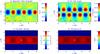 |
Fig. 1 Low-density model: a) magnetic field strength; b) perturbation of the B-LOS angle; c) thermal and nonthermal number density; and d) temperature perturbations along a cross section through the center of the cylinder. Snapshots are taken at t = 3 / 4P with a viewing angle 90°. The black (white) cross indicates the antinode (node) of the field magnitude, density, and temperature oscillation. The lines of sight passing upward through the antinode (node) at different viewing angles, 30°, 45°, 60°, and 90°, are shown by dashed lines in plot a b). (A color version of this figure is available in the online journal.) |
It is important to mention that perturbations of the direction of the magnetic field vector B cause a variation of the angle θ between the line of sight and B (B-LOS angle), which leads to an additional modulation of the GS emission. The B-LOS angle is determined in Cartesian coordinates: 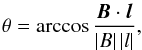 (1)where B is directed toward the positive Z-axis in the equlibrium state and l is a unit vector determining the direction of the line of sight in the YZ-plane.
2.2. Nonthermal electrons
In both models the cylinder is filled with nonthermal mildly relativistic electrons, whose perturbation is proportional to the thermal plasma density. The non-thermal electron distribution is described by the analytical function G(E,μ), which is written in the factorized form: 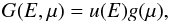 (2)which is a product of the energy distribution function u(E) and the angular distribution function g(μ). Here, μ = cosα, where α is the electron pitch angle (i.e., the angle between the electron momentum and the magnetic field vector). Reznikova et al. (2014) reported the results for a single power-law distribution on energy and isotropic pitch-angle distribution. Using these simple distributions enabled us to compare the obtained dependence with the analytical approximation of Dulk (1985). A single power-law spectrum was taken with a low cutoff energy Emin = 0.1 MeV. However, hard X-ray observations show that in real flares there are many electrons with lower energies E< 0.1 MeV. Although the GS radiation from these electrons is negligible, they can still influence self-absorption and Razin suppression. Therefore, we considered a more realistic double power-law spectrum in our current work, described by the following expression:
 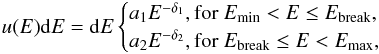 (3)where the electron spectral indexes for the low-energy part δ1 = 1.5, and for the high-energy part δ2 = 3, the lowest energy Emin = 0.01 MeV, the highest energy Emax = 10 MeV, and the break point Ebreak = 0.5 MeV. To make the function continuous in the above expression, we took
  . The normalization factor is given by
  (4)where Nbi = NPi/ 4000 is the internal nonthermal number density at E ≥ Ebreak and the external nonthermal number density Nbe = 0. This yields Nbi one order of magnitude lower than the thermal density at E ≥ 0.01 MeV. The distribution over pitch-angle is isotropic: g(μ) = const. = 1 / 2.
2.3. GS codes
To calculate the circular polarization of microwave emission, we used the GS code of Fleishman & Kuznetsov with radiation transfer (Kuznetsov et al. 2011)1. The output of this code are arrays of the spectral intensities of the left- and right-polarized emission components, IL and IR, as a function of the observed frequency, f. They are calculated by numerical integration of the radiation transfer equation:  (5)along each selected line of sight. Here, l is the coordinate along the line of sight, jL and jR are the corresponding GS emissivities, and κL and κR are the absorption coefficients. The source volume is divided into a number of volume elements (voxels); each voxel is considered to be quasi-homogeneous by approximating the plasma properties in a voxel on their mean. Left-polarized emission corresponds to either an ordinary or extraordinary magnetoionic mode, depending on the magnetic field direction, and right-polarized emission corresponds to the opposite mode.
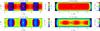 |
Fig. 2 Polarization (Stokes V) of the radiation from the loop observed at angles of (left column) 90° and (right column) 60° at frequencies 2.5 GHz and 10 GHz. Snapshots are taken at t = 3P/ 4 for the base model. Left and right crosses denote the location of an antinode and node, respectively. A pixel of size 0.5′′ (dotted line) is shown in the bottom panels. |
At low frequencies, GS emission can show an oscillatory (harmonic) spectral structure (see, e.g., Ramaty 1969; Holman 2003). However, here we used the continuous algorithm for calculating the GS emission (Fleishman & Kuznetsov 2010), which does not reproduce the harmonic structure. This approximation was chosen because: a) it greatly accelerates the calculations; b) in real flaring loops, the harmonic spectral structure of the observed emission is usually smoothed as a result of source inhomogeneity and limited spatial resolution of an instrument (Kuznetsov et al. 2011); c) we are primarily interested in the phase relations, therefor the averaged continuous spectra is sufficient.
The code includes mode coupling effects, that are interactions between two modes in the areas of the transverse magnetic field (Cohen 1960; Zheleznyakov & Zlotnik 1964; Zheleznyakov 1996). In this a case, the dispersion curves of the O-mode and X-mode approach each other, and transition of an electromagnetic wave from one dispersion curve to another is possible. The coupling effect is detectable on the polarization as a possible change of the polarization in these areas.
Intensities are calculated under the assumption that the emission source is observed from the distance of one astronomical unit, that is, located at the Sun and observed from the Earth. Outside the flaring loop, the emission propagates as it does in a vacuum.
To calculate the optical depth,  , we used an earlier version of the GS code of Fleishman & Kuznetsov (Fleishman & Kuznetsov 2010). This version computes the output plasma emissivities jo,x and absorption coefficients κo,x for the ordinary and extraordinary modes for each voxel on the line of sight.
Although free-free emission contribution is very small in the flare scenario, it is also accounted for in both versions of the code.
3. Calculation results
The circular polarization (parameter Stokes V) of the loop at frequency f in the image plane (x,y) at time t and specific view angles is obtained as  (6)where Rf is the right-polarized emission intensity and IL is the left-polarized emission intensity. Another important characteristic, the circular polarization degree, which is frequently used to judge the emission mechanism and/or derive the magnetic field strength, is defined as
 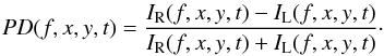 (7)The lowest value of this quantity is −1 (perfectly left-handed circular polarization), and highest is + 1 (perfectly right-handed circular polarization).
Both quantities, (6) and (7), were calculated at three viewing angles relative to the cylinder axis, 60°, 45°, and 30° and at twelve frequencies between 1 GHz and 100 GHz. For a 90° viewing angle, all four Stokes parameters (I,Q,U,V) were calculated to obtain circulary and lineary polarised components because the latter component is important for the quasi-perpendicular layer. Furthermore we integrated the intensity over pixels of sizes 0.5′′ to imitate angular resolution of a radioheliograph, such as ALMA. This resolution equals λ/ 8 of longitudinal wave length λ = 2π/k = 2.8 Mm of the sausage mode. As Reznikova et al. (2014) showed, a spatial resolution better than λ/ 8 is not necessary. However, reducing the resolution to 2.8′′ (or 0.7λ) decreases the modulation depth by more than a factor of four compared with 0.5′′.
3.1. Spacial structure of the polarization
First, we show the results obtained for the base model. Here, the Razin frequency, fR ≈ 20NP/B⊥, varies from 4 GHz to 8 GHz when the viewing angle changes from 90° to 30°. Therefore, the low-frequency part of the GS spectrum will be affected by Razin suppression (Razin 1960a,b).
Figure 2 shows the polarization (Stokes V) observed for the base model at viewing angles 90° and 60°, and Fig. 3 at angles 45° and 30°. The polarization is shown at frequencies (top) of 2.5 GHz and (bottom) 10 GHz, which represents the two characteristic cases of low (f<fpeak) and high frequency (f>fpeak) emission. Images of the polarization show a smooth transition in frequency from 2.5 to 10 GHz. Therefore, we do not present an image at the peak frequency, fpeak = 5 GHz. Because the nonthermal number density outside the loop Nbe is zero, this area is not shown. The snapshots are taken at three quarters of the period, coinciding with that of Fig. 1.
Interestingly, for a 90° viewing angle, positively and negatively polarized areas of the loop alternate. The number of alterations along the loop is equal to the harmonics number. The boundary between different polarization signs passes through an antinode. Strictly speaking, in a quasi-transverse layer (θ ≈ 90°) linear polarization arises in addition to a circularly polarised component (Ramaty 1969). However, because of the differential Faraday rotation, linear polarization of the solar microwave emission has been detected only rarely (Alissandrakis & Chiuderi-Drago 1994). To the left of the boundary marked by a black cross, the B-LOS angle θ< 90° and to the right θ> 90° on the observer’s side of the cylinder. Consequently, the projection of the magnetic field vector on the line of sight, BLOS = Bcosθ, changes its sign on this boundary. Positive (right-handed) polarization V corresponds to the positive BLOS and negative (left-handed) polarization corresponds to the negative BLOS. Therefore, the extraordinary mode is emitted. For other viewing angles, 60° (Fig. 2 right), 45° and 30° (Fig. 3 left and right), the polarization is always positive because the B-LOS angle is always θ< 90°. This finding agrees with the theory that the polarization of GS and free-free emission should be in the sense of the X-mode in the optically thin regime (Dulk 1985). As a result of Razin suppression in the base model, the cylinder is optically thin at all examined frequencies. The optical depth of the emitting source is shown in Fig. 4. The optical depth τ for both modes in the base model at all studied frequencies is lower than unity.
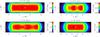 |
Fig. 3 Polarization (Stokes V) of the radiation from the loop observed at the viewing angles (left column) 45° and (right column) 30°. Same as Fig. 2. The location of an antinode and node are shown by black and whight crosses, respectively. A pixel of size 0.5′′ (dotted line) is shown in the bottom panels. |
For 60° and 45°, the polarization variation along the cylinder is more pronounced at high frequency (10 GHz) than at low frequency (2.5 GHz). The observed brightness minimum coincides with the antinode location denoted by the black cross, the area of weaker magnetic field strength and density at t = 3P/ 4. However, it is the reverse for the 30° case. This is because the spatial variation of the B-LOS angle becomes more significant with decreasing viewing angles. The spatial distribution of the polarization has similar patterns to that found for the intensity (see Reznikova et al. 2014).
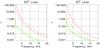 |
Fig. 4 Optical depth of the emitting source along the lines of sight that crosses the antinode at two different viewing angles for the base model (solid for the X-mode and dotted for the O-mode) and for the low-density model (dashed for the X-mode and dashed-doted for the O-mode). |
Figures 5 and 6 show the polarization distribution for the low-density model, in which Razin suppression does not influence the low-frequency (f<fpeak) part of the spectrum. Therefore, the emitting source should be optically thick at low frequencies. Again, we observe a switch of the polarization sign at 90° and positive polarization for other angles. The exception is 2.5 GHz observed at a 60° viewing angle, where negative polarization is found for the main body of the loop. This agrees with the theory that in the optically thick regime the extraordinary mode of GS emission is absorbed more efficiently and the ordinary mode of GS emission should be observed (see, for example Zheleznyakov 1996). However, for 45° and 30° angles, the polarization sign is not negative at 2.5 GHz. This fact is difficult to explain, since judging from the spectrum, one would expect the 2.5 GHz loop to be optically thick in both cases: the peak frequency is located at 5 GHz (see Fig. 7).
This puzzle can be solved by examining the optical depth for the low-density model, shown in Fig. 4 by the dashed curve for the X-mode and by the dashed-dotted curve for the O-mode. For 60°, the values of τo and τx are higher than unity at 2.5 GHz. Therefore, the source is optically thick for both modes, and the ordinary mode is generated. For a 45° angle, the optical depths for the O-mode τ° ≈ 1 at 2.5 GHz corresponds to almost zero polarization. For a 30° angle, τ°< 1 at 2.5 GHz and therefore, the polarization grows again and becomes positive. Interestingly, the peak frequencies in the polarization spectra correspond to τx = 1.
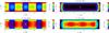 |
Fig. 5 Polarization (Stokes V) of the radiation in the low-density model. The loop is observed at angles of (left column) 90° and (right column) 60° at frequencies 2.5 GHz and 10 GHz. |
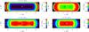 |
Fig. 6 Polarization (Stokes V) of the radiation in the low-density model. The loop is observed at angles of (left column) 45° and (right column) 30° at frequencies 2.5 GHz and 10 GHz. |
3.2. Temporal variation of the polarization
The intensity, polarization (Stokes V), and circular polarization degree (Stokes V/I) spectra on the LOS crossing an antinode are shown in Fig. 7 for the base model and in Fig. 8 for the low-density model at times P/ 4 (dashed) and 3P/ 4 (dashed-dotted) of the mode period P. The spectra were obtained with a spatial resolution of 0.5′′ to imitate future observations with ALMA. An increase of all three quantities, intensity, I, polarization, V, and polarization degree, PD near the spectral peak and higher frequencies at one quarter of the period is clearly seen at the 60° viewing angle. At this moment, the magnetic field and nonthermal density are highest for this antinode. For 30° the intensity and polarization show the opposite behavior near the peak in the base model and almost no variation in the low-density model. For a viewing angle of 90° (not shown) an antinode corresponds to the border between positive and negative polarities, and averaging over a 0.5′′ pixel gives zero polarization.
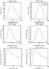 |
Fig. 7 Base model: spatially resolved emission spectra of intensity (top row), polarization (middle row), and polarization degree (bottom row). Emission is integrated over a pixel of 0.5′′ centered on an antinode of the cylinder observed at an angle of 60° (left) and 30° (right) at times P/ 4 (dashed) and 3P/ 4 (dashed-dotted) of the mode period P. |
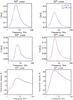 |
Fig. 8 Low-density model: spatially resolved emission spectra of intensity (top row), polarization (middle row), and polarization degree (bottom row). Emission is integrated over a pixel of 0.5′′ centered on an antinode of the cylinder observed at an angle of 60° (left) and 30° (right) at times P/ 4 (dashed) and 3P/ 4 (dashed-dotted) of the mode period P. |
We compared our results with the famous approximations made by Dulk (1985). According to their empirical expressions, in the optically thin regime (τ ≪ 1), the dependence of the polarization degree PD on the spectral index δ, and the B-LOS angle θ, is 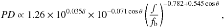 (8)where the gyrofrequency fb = qB/m, q and m are the electron charge and mass.
The approximation is made for a single power-law energy spectrum of electrons. Because the high-energy electrons have the highest efficiency to radiate GS emission, we took the electron spectral index δ = 3 similar to the index for the high-energy part in our model. This yields a polarization degree at 10 GHz, where the cylinder is optically thin in both models: 17% (30%) and 37% (53%) for the equilibrium parameters in the base (low density) model for viewing angles 60° and 30°, respectively. These estimates agree with the simulated polarization degree of emission at 10 GHz.
Since the parameters averaged along the LOS that cross the node are constant with time, the modulation of the circular polarization V and polarization degree PD = V/I is negligible at all viewing angles except 90°. Emission spectra corresponding to the latter case are shown in Fig. 10 for the base model. The circular polarization degree at t = P/ 4 reaches 45% at 6 GHz for the best spatial resolution in our model (0.03′′), and it drops to 38% for a resolution of 0.5′′. Both quantities, V and PD, reverse their sign at t = P/ 2 when a radius expansion changes to compression, and therefore the BLOS component of the field vector becomes negative in the part of the cylinder that is nearest to an observer. The reversal of the spectra is only associated with the temporal variation of the B-LOS angle: it changes from acute to obtuse in the middle of the period.
The polarization reversal phenomenon is found for both models and at all examined frequencies. This phenomenon could be detected in observations for the flaring loop located on the limb if it is seen at 90° ± 2° (± 1°) in the base (low density) model, which would appear to be a rare case. However, even if part of the oscillating loop is observed at a LOS angle of 90°, again, one would expect to observe a periodical switch of the V and PD sign in this part. In this case, their modulation depth can reach 100%.
It should be noted, however, that the spectrum observed on Earth will strongly depend on the conditions outside the emitting source. According to the mode-coupling theory in a magnetized plasma (see Zheleznyakov 1996), both ordinary and extraordinary modes become linear when passing through a transverse magnetic field layer (θ ≈ 90°). When leaving it, they may reverse the rotation direction for weak mode-coupling or remain unchanged for strong coupling. The type and degree of coupling depends on the conditions outside the emitting loop (magnetic field direction and strength, density, observed frequency). In our model, the emission generated inside the flare loop propagates directly into the vacuum, and the real solar spectrum can differ from the one obtained in the calculations.
Another important type of polarization in a quasi-transverse layer is linear polarization. Therefore, all four Stokes parameters (I,Q,U,V) were calculated for the LOS angle 90°. In Fig. 9, right plot, we show the total linear polarization degree  . The spectrum was obtained with a spatial resolution of 0.5′′. Such a high spatial resolution for solar observations will be reached by ALMA and is necessary to avoid the influence of the differential Faraday rotation when detecting a linear polarization. Although the radioheliograph ALMA has a sufficient resolution in space and frequencies, the linear polarization degree tends to zero in the frequency range of the instrument (f> 85 GHz). It is sufficiently high in the frequency range of the EOVSA array (>50% at 2.5 GHz). However, Kuznetsov (2011) found that the limiting factor for this instrument is the spatial resolution, which has to be better than 1′′.
We estimated the modulation depth of the circular polarization on the line of sight that crosses the antinode. This quantity is calculated as δV/V0 = (V(t) − V0) /V0, where V(t) is the time series of the polarization at the selected frequency f, and V0 is the corresponding equilibrium value. Figure 10 represents the modulation depth of the parameter Stokes V (top row) and Stokes V/I (bottom row) in the base model.
The phase relations are the same as found earlier for the intensity variation by Reznikova et al. (2014). The oscillation at 60° at all frequencies is found to be inphase with the averaged variation of the magnetic field strength and density. However, at 45°, the emission at 2.5 GHz oscillates in antiphase to B and N; for a 30° angle this is true for all frequencies. As a result of an antiphase with magnetic field and density perturbations of the angle θ, the modulation depth of the polarization strongly decreased at angles 45° and even inverted the phase at an angle of 30°. The modulation depth δV/V at frequency 10 GHz is 10% at a viewing angle of 60°, 5% at 45° and lower than 1% at 30°. The Razin effect at low frequency enhances the relative amplitude of the modulation, although the absolute flux increase is quiet small. This corresponds to the average along the LOS perturbations of the magnetic field δB/B of 2.5%, 2%, and 1%.
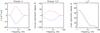 |
Fig. 9 Spatially resolved emission spectra corresponding to the LOS crossing a node of the cylinder observed at an angle of 90°. From left to right: polarization (Stokes V), circular polarization degree (Stokes V/I), and the total linear polarization degree |
The PD at three examined frequencies (2.5, 5, 10 GHz) varies in phase with the magnetic field. This is also true for the low-density model shown in Fig. 11. Indeed, Eq. (8) shows that the circular polarization degree PD variations in the optically thin part of the spectra must occur in phase with B and in antiphase with the angle θ perturbations (θ> 0). The highest modulation depth is found at 10 GHz: 3.4% (2.2%), 3% (1.9%), and 1.4% (0.8%) at 60°, 45°, and 30° in the base (low density) model. If we take the average along the LOS perturbations of the magnetic field and angle shown in Fig. 10 and δ = 3, then Eq. (8) yields the following modulation depth of the PD on the LOS crossing an antinode at 10 GHz: 3.2% (2.1%), 2.8 (1.8%), and 1.7% (0.8%) for the base (low density) model, which is very close to our findings.
4. Conclusions
We studied the modulation of the microwave flaring polarization (GS and free-free) by the standing fast sausage wave using a linear 3D MHD model of a plasma cylinder. The modulation was investigated for two sets of typical flaring parameters: the base model with the Razin suppression at low frequencies (f<fpeak), and the low-density model in which the Razin effect was negligible at all examined frequencies (1–100 GHz). The temporal circular polarization variation was analyzed on the LOS crossing an antinode and a node of the field and density variation for different viewing angles.
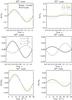 |
Fig. 10 Temporal variation of the normalized polarization (top row) and polarization degree (bottom row) from a pixel of 0.5′′ centered on an antinode in the base model. The color coding of different frequencies is denoted in the top-right plot. The relative perturbations of the magnetic field, density, and B-LOS angle averaged along the LOS (second row) are shown by solid, dotted, and dashed-dotted curves, respectively. |
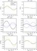 |
Fig. 11 Same as in Fig. 10, but for the low-density model. Dashed and dash-dot-dot lines indicate relative perturbations of the magnetic field and B-LOS angle near the cylinder surface at the point of intersection with the LOS. |
For the LOS crossing an antinode, we found that in absolute value the circular polarization (Stokes V) oscillation is in phase with the intensity oscillation described in Reznikova et al. (2014). This finding agrees with previous predictions (Mossessian & Fleishman 2012). The polarization degree PD oscillates in phase with the magnetic field at examined frequencies (2.5, 5, 10 GHz) in both models. The highest variation amplitude is found near the spectral maximum (5, 10 GHz) if observed at a 60° viewing angle: the modulation depth is 10% (7.5%) for the Stokes V parameter and 3.5% (2%) for the polarization degree in the base (low density) model. If observed at 30°, it decreases to about 1%.
For example, if the period of the observed QPP indicates a fundamental sausage mode, the antinode location corresponds to the loop apex. Therefore, if the loop top is observed at a large viewing angle (≥60°), one would expect to find in-phase oscillations between Stokes I, an absolute value of Stokes V, and polarization degree. In-phase variations are also expected between the microwave flaring emission at low (f<fpeak) and high (f>fpeak) frequencies. The latter is true provided that emitting electrons are distributed more or less uniformly along the entire loop cross-section in the equilibrium state. In our artificial observations we showed that a spatial resolution better than λ/ 8 of longitudinal wave length λ of the sausage mode is not necessary. Therefore, for a fundamental mode, the resolution L/ 4 of the loop length L would meet the requirements. The length L can roughly vary between 10′′ and 100′′. Therefore, the Nobeyama Radioheliograph has sufficient resolution at 17 GHz for most large flaring loops, and the future instruments EOVSA, CSRH, and ALMA have it for almost all sizes.
For the LOS that crosses a node, the variations of the circular polarization (Stokes V) and polarization degree (Stokes V/I) are negligible, except when the LOS angle equals 90°. We found the periodical reversal of the polarization and polarization degree spectra with period equal to P/ 2 of the sausage wave period P. In this case, the modulation depth of both quantities reaches 100%. This phenomenon is due to the radius variation that leads to a change in the sign of the magnetic field vector projection on the line of sight. It can be taken into account when interpreting oscillations as a sausage mode. In the part of the loop seen at a LOS angle of 90°, one would expect to observe a periodic switch of the circular polarization and polarization degree signs. For the limb loop observed at 90° ± 2° (±1°) in the base (low-density) model this switch should appear in both time and space. A number of alterations along the loop equals the harmonics number. However, the polarization observed at Earth in this case can be determined not only by the direction of the magnetic field of the emission loop, but also by the propagation conditions in the corona outside the radiating source.
The code and documentation are available at https://sites.google.com/site/fgscodes/transfer
Acknowledgments
We acknowledge funding from the Odysseus Programme of the FWO Vlaanderen and from the EU’s 7th Framework Programme as an ERG with grant number 276808. The research carried out by A.A.K. is partly supported by Marie Curie International Research Staff Exchange Scheme “Radiosun” (PEOPLE-2011-IRSES-295272) and the Russian Foundation of Basic Research (grants 13-02-90472 and 14-02-91157). This research is in the frame of the Belspo IAP P7/08 CHARM network and the GOA-2015-014 (KU Leuven). We are thankful to an anonymous referee for suggesting improvements to an earlier version of this paper.
References
- Alissandrakis, C. E., & Chiuderi-Drago, F. 1994, ApJ, 428, L73 [NASA ADS] [CrossRef] [Google Scholar]
- Antolin, P., & Van Doorsselaere, T. 2013, A&A, 555, A74 [NASA ADS] [CrossRef] [EDP Sciences] [Google Scholar]
- Banerjee, D., Erdélyi, R., Oliver, R., & O’Shea, E. 2007, Sol. Phys., 246, 3 [NASA ADS] [CrossRef] [Google Scholar]
- Cohen, M. H. 1960, ApJ, 131, 664 [NASA ADS] [CrossRef] [Google Scholar]
- De Moortel, I., & Nakariakov, V. M. 2012, Phil. Trans. R. Soc. A, 370, 3193 [NASA ADS] [CrossRef] [Google Scholar]
- Dulk, G. A. 1985, ARA&A, 23, 169 [NASA ADS] [CrossRef] [Google Scholar]
- Fleishman, G. D., & Kuznetsov, A. A. 2010, ApJ, 721, 1127 [NASA ADS] [CrossRef] [Google Scholar]
- Fleishman, G. D., & Melnikov, V. F. 2003, ApJ, 587, 823 [NASA ADS] [CrossRef] [Google Scholar]
- Gary, Dale E., Nita, G. M., & Sane, N. 2012, A&AS Meeting, 220, 204.30 [Google Scholar]
- Grechnev, V. V., Lesovoi, S. V., Smolkov, G. Ya., et al. 2003, Sol. Phys., 216, 239 [Google Scholar]
- Holman, G. D. 2003, ApJ, 586, 606 [NASA ADS] [CrossRef] [Google Scholar]
- Inglis, A. R., Nakariakov, V. M., & Melnikov, V. F. 2008, A&A, 487, 1147 [NASA ADS] [CrossRef] [EDP Sciences] [Google Scholar]
- Inglis, A. R., Van Doorsselaere, T., Brady, C. S., & Nakariakov, V. M. 2009, A&A, 503, 569 [NASA ADS] [CrossRef] [EDP Sciences] [Google Scholar]
- Kopylova, Y. G., Stepanov, A. V., & Tsap, Y. T. 2002, Astron. Lett., 28, 783 [NASA ADS] [CrossRef] [Google Scholar]
- Kupriyanova, E. G., Melnikov, V. F., Nakariakov, V. M., & Shibasaki, K. 2010, Sol. Phys., 267, 329 [NASA ADS] [CrossRef] [Google Scholar]
- Kuznetsov, A. A. 2011, EPSC Abstracts, Vol. 6, EPSC-DPS2011-500 [Google Scholar]
- Kuznetsov, A. A., Nita, G. M., & Fleishman, G. D. 2011, ApJ, 742, 87 [NASA ADS] [CrossRef] [Google Scholar]
- Lesovoi, S., Altyntsev, A., Ivanov, E., & Gubin, A. 2012, Sol. Phys., 280, 651 [NASA ADS] [CrossRef] [Google Scholar]
- Melnikov, V. F., Reznikova, V. E., Shibasaki, K., & Nakariakov, V. M. 2005, A&A, 439, 727 [NASA ADS] [CrossRef] [EDP Sciences] [Google Scholar]
- Mossessian, G., & Fleishman, G. D. 2012, ApJ, 748, 140 [NASA ADS] [CrossRef] [Google Scholar]
- Nakariakov, V. M., & Verwichte, E. 2005, Liv. Rev. Sol. Phys., 2, 3 [Google Scholar]
- Nakajima, H., Nishio, M., Enome, S., et al. 1994, IEEE Proc., 82, 705 [NASA ADS] [CrossRef] [Google Scholar]
- Nakariakov, V. M., & Melnikov, V. F. 2009, Space Sci. Rev., 149, 119 [NASA ADS] [CrossRef] [Google Scholar]
- Nakariakov, V. M., Melnikov, V. F., & Reznikova, V. E. 2003, A&A, 412, L7 [NASA ADS] [CrossRef] [EDP Sciences] [Google Scholar]
- Nakariakov, V. M., Hornsey, C., & Melnikov, V. F. 2012, ApJ, 761, 134 [NASA ADS] [CrossRef] [Google Scholar]
- Ramaty, R. 1969, ApJ, 158, 753 [NASA ADS] [CrossRef] [Google Scholar]
- Razin, V. A. 1960a, Izv. VUZov Radiofizika, 3, 584 [Google Scholar]
- Razin, V. A. 1960b, Izv. VUZov Radiofizika, 3, 921 [Google Scholar]
- Reznikova, V. E., Melnikov, V. F., Su, Y., & Huang, G. 2007, Astron. Rep., 51, 588 [NASA ADS] [CrossRef] [Google Scholar]
- Reznikova, V. E., Antolin, P., & Van Doorsselaere, T. 2014, ApJ, 785, 86 [NASA ADS] [CrossRef] [Google Scholar]
- Rosenberg, H. 1970, A&A, 9, 159 [NASA ADS] [Google Scholar]
- Stepanov, A. V., Kopylova, Yu. G., Tsap, Yu. T., et al. 2004, Astron. Lett., 30, 480 [NASA ADS] [CrossRef] [Google Scholar]
- Stix, T. H. 1962, The theory of plasma waves (New York: McGraw-Hill) [Google Scholar]
- Van Doorsselaere, T., De Groof, A., Zender, J., Berghmans, D., & Goossens, M. 2011, ApJ, 740, 90 [NASA ADS] [CrossRef] [Google Scholar]
- Vasheghani Farahani, S., Hornsey, C., Van Doorsselaere, T., & Goossens, M. 2014, ApJ, 781, 92 [NASA ADS] [CrossRef] [Google Scholar]
- Yan, Y., Wang, W., Liu, F., et al. 2013, International Astronomical Union 2013, DOI: 10.1017/S1743921313003001 [Google Scholar]
- Zheleznyakov, V. V. 1996, Radiation in Astrophysical Plasmas (Kluwer academic publishers) [Google Scholar]
- Zheleznyakov, V. V., & Zlotnik, E. Ya. 1964, Sov. Astron., 7, 485 [NASA ADS] [Google Scholar]
All Tables
All Figures
|
Fig. 1 Low-density model: a) magnetic field strength; b) perturbation of the B-LOS angle; c) thermal and nonthermal number density; and d) temperature perturbations along a cross section through the center of the cylinder. Snapshots are taken at t = 3 / 4P with a viewing angle 90°. The black (white) cross indicates the antinode (node) of the field magnitude, density, and temperature oscillation. The lines of sight passing upward through the antinode (node) at different viewing angles, 30°, 45°, 60°, and 90°, are shown by dashed lines in plot a b). (A color version of this figure is available in the online journal.) |
| In the text | |
|
Fig. 2 Polarization (Stokes V) of the radiation from the loop observed at angles of (left column) 90° and (right column) 60° at frequencies 2.5 GHz and 10 GHz. Snapshots are taken at t = 3P/ 4 for the base model. Left and right crosses denote the location of an antinode and node, respectively. A pixel of size 0.5′′ (dotted line) is shown in the bottom panels. |
| In the text | |
|
Fig. 3 Polarization (Stokes V) of the radiation from the loop observed at the viewing angles (left column) 45° and (right column) 30°. Same as Fig. 2. The location of an antinode and node are shown by black and whight crosses, respectively. A pixel of size 0.5′′ (dotted line) is shown in the bottom panels. |
| In the text | |
|
Fig. 4 Optical depth of the emitting source along the lines of sight that crosses the antinode at two different viewing angles for the base model (solid for the X-mode and dotted for the O-mode) and for the low-density model (dashed for the X-mode and dashed-doted for the O-mode). |
| In the text | |
|
Fig. 5 Polarization (Stokes V) of the radiation in the low-density model. The loop is observed at angles of (left column) 90° and (right column) 60° at frequencies 2.5 GHz and 10 GHz. |
| In the text | |
|
Fig. 6 Polarization (Stokes V) of the radiation in the low-density model. The loop is observed at angles of (left column) 45° and (right column) 30° at frequencies 2.5 GHz and 10 GHz. |
| In the text | |
|
Fig. 7 Base model: spatially resolved emission spectra of intensity (top row), polarization (middle row), and polarization degree (bottom row). Emission is integrated over a pixel of 0.5′′ centered on an antinode of the cylinder observed at an angle of 60° (left) and 30° (right) at times P/ 4 (dashed) and 3P/ 4 (dashed-dotted) of the mode period P. |
| In the text | |
|
Fig. 8 Low-density model: spatially resolved emission spectra of intensity (top row), polarization (middle row), and polarization degree (bottom row). Emission is integrated over a pixel of 0.5′′ centered on an antinode of the cylinder observed at an angle of 60° (left) and 30° (right) at times P/ 4 (dashed) and 3P/ 4 (dashed-dotted) of the mode period P. |
| In the text | |
|
Fig. 9 Spatially resolved emission spectra corresponding to the LOS crossing a node of the cylinder observed at an angle of 90°. From left to right: polarization (Stokes V), circular polarization degree (Stokes V/I), and the total linear polarization degree |
| In the text | |
|
Fig. 10 Temporal variation of the normalized polarization (top row) and polarization degree (bottom row) from a pixel of 0.5′′ centered on an antinode in the base model. The color coding of different frequencies is denoted in the top-right plot. The relative perturbations of the magnetic field, density, and B-LOS angle averaged along the LOS (second row) are shown by solid, dotted, and dashed-dotted curves, respectively. |
| In the text | |
|
Fig. 11 Same as in Fig. 10, but for the low-density model. Dashed and dash-dot-dot lines indicate relative perturbations of the magnetic field and B-LOS angle near the cylinder surface at the point of intersection with the LOS. |
| In the text | |
Current usage metrics show cumulative count of Article Views (full-text article views including HTML views, PDF and ePub downloads, according to the available data) and Abstracts Views on Vision4Press platform.
Data correspond to usage on the plateform after 2015. The current usage metrics is available 48-96 hours after online publication and is updated daily on week days.
Initial download of the metrics may take a while.