| Issue |
A&A
Volume 574, February 2015
|
|
|---|---|---|
| Article Number | A10 | |
| Number of page(s) | 7 | |
| Section | Astrophysical processes | |
| DOI | https://doi.org/10.1051/0004-6361/201424919 | |
| Published online | 16 January 2015 | |
Rossby wave instability does not require sharp resistivity gradients⋆
1 Jet Propulsion Laboratory, California Institute of Technology, 4800 Oak Grove Drive, Pasadena, CA 91109, USA
e-mail: This email address is being protected from spambots. You need JavaScript enabled to view it.
2 Department of Geology and Planetary Sciences, California Institute of Technology, 1200 E. California Ave, Pasadena, CA 91125, USA
3 Niels Bohr International Academy, Niels Bohr Institute, Blegdamsvej 17, 2100 Copenhagen, Denmark
Received: 4 September 2014
Accepted: 30 October 2014
Abstract
Context. Rossby wave instability (RWI) at dead zone boundaries may play an important role in planet formation. Viscous hydrodynamics results suggest RWI is excited only when the viscosity changes over a radial distance less than two density scale heights. However in the disks around Solar-mass T Tauri stars, it is not viscosity but magnetic forces that provide the accretion stress beyond about 10 AU, where surface densities are low enough so stellar X-rays and interstellar cosmic rays can penetrate.
Aims. We explore the conditions for RWI in the smooth transition with increasing distance, from resistive and magnetically-dead to conducting and magnetically-active.
Methods. We perform 3D unstratified MHD simulations with the Pencil code, using static resistivity profiles.
Results. We find that in MHD, contrary to viscous models, the RWI is triggered even with a gradual change in resistivity extending from 10 to 40 AU (i.e., spanning 15 scale heights for aspect ratio 0.1). This is because magneto-rotational turbulence sets in abruptly when the resistivity reaches a threshold level. At higher resistivities the longest unstable wavelength is quenched, resulting in a sharp decline of the Maxwell stress towards the star. The sharp gradient in the magnetic forces leads to a localized density bump, that is in turn Rossby wave unstable.
Conclusions. Even weak gradients in the resistivity can lead to sharp transitions in the Maxwell stress. As a result the RWI is more easily activated in the outer disk than previously thought. Rossby vortices at the outer dead zone boundary thus could underlie the dust asymmetries seen in the outer reaches of transition disks.
Key words: accretion, accretion disks / planets and satellites: formation / instabilities / magnetohydrodynamics (MHD) / turbulence / methods: numerical
A movie associated to Fig. 4 is available in electronic form at http://www.aanda.org
Carl Sagan Fellow.
Marie Curie Fellow.
© ESO, 2015
1. Introduction
The Rossby wave instability (RWI; Lovelace & Hohfeld 1978; Toomre 1981; Papaloizou & Pringle 1984, 1985) is a non-axisymmetric hydrodynamic shear instability associated with axisymmetric extrema of vortensity (Lovelace et al. 1999; Li et al. 2000). The localized extremum behaves as a potential well that, if deep enough, can trap modes in its corotational resonance. The trapped modes are linearly unstable and eventually saturate into large-scale vortices (Hawley 1987; Li et al. 2001; Tagger 2001). Essentially, the RWI is the form the Kelvin-Helmholtz instability takes in differentially rotating disks, with the upshot being the conversion of the surplus shear into vorticity.
The RWI was originally proposed in the context of galaxies (Lovelace & Hohfeld 1978), and later, in accretion disk tori (Papaloizou & Pringle 1984,1985). First sought as the elusive source of accretion in disks, the interest in it decreased after the discovery of the magnetorotational instability (MRI, Balbus & Hawley 1991). It has been reintroduced in the protoplanetary disk landscape by Varnière & Tagger (2006) who suggested that the RWI would naturally develop in the transition between poorly ionized zones that are “dead” to the MRI, and the magnetized zones, “active” to the MRI. This is because the transition constitues a gradient in turbulent viscosity, that in turn would lead to RWI-unstable density bumps at the dead zone boundaries.
Subsequently, Lyra et al. (2008b, 2009a,b) presented proof-of-concept models showing that the particle concentration in these vortices is strong enough to assemble bound clumps of solids, in the Mars-mass range. Although those models were idealized (2D, no collisional fragmentation of the particles), they showed for the first time that planet formation was feasible in physically-motivated vortices. This scenario has since been shown to hold as increasing sophistication is sought. The RWI was shown to exist in three dimensions with vertical stratification in barotropic (Meheut et al. 2010, 2012a,b), polytropic (Lin 2012a), non-barotropic (Lin 2013), and self-gravitating disks (Lin 2012b). Vortices have also been studied in local models, that can more easily afford high resolution, showing that the “elliptic instability” that destroys an isolated vortex (Kerswell 2002; Lesur & Papaloizou 2009) is well balanced by a vorticity source, leading to vortex survival (Lesur & Papaloizou 2010; Lyra & Klahr 2011).
A critical test was to replace the alpha viscosity approximation (Shakura & Sunyaev 1973) by magnetohydrodynamics (MHD), with a properly modeled active zone. This was done by Lyra & Mac Low (2012) who replaced the jump in alpha viscosity by a jump in resistivity, letting the MRI naturally evolve in the active zone. The RWI was excited, leading to a vortex in the dead side of the transition. This result was confirmed by Faure et al. (2014), with a dynamically-varying resistivity profile in a thermodynamically-evolving disk.
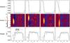 |
Fig. 1 Suite of MHD simulations. From left to right, the transition width is h1 = 0.1, 0.2, 0.4 and 0.8. The resulting resistivity profiles are shown in the upper panels. The dashed vertical lines correspond to 2H around the jump center at r = 2.5. The model with h1 = 0.8 corresponds to a smooth jump from r ≈ 1 to r ≈ 4, i.e., over ≈15 scale heights. Although at different times, all models develop a sharp density bump that goes unstable to the RWI, producing a Rossby vortex (middle panels). The panels, from left to right, correspond to density snapshots at 100, 100, 122, and 232T0, where T0 is the orbital period at r = 1. The dashed vertical lines correspond to 2H around the density maximum. The reason for RWI excitation in these cases is because even though the resistivity jump is smooth, the transition in Maxwell stress remains sharp (lower panels). The transition in Reynolds stress is somewhat smoother, but turbulent stresses do not blur gradients in the same way Laplacian viscosity does, and the density bump remains RWI-unstable. |
One of the remaining questions toward more realism in this scenario is how sharp does the transition need to be, and how realistic is it to expect such a gradient. Although linear theory predicts that any extremum of vortensity is unstable to the RWI, one finds in practice that the extremum has to be sharp enough to trap modes in the corotational resonance. The required width is problem-dependent, but as a rule-of-thumb, Li et al. (2000) find that a 10%−20% radial variation in density over a length scale comparable to the pressure scale height (H) is sufficient to trigger it. Lyra et al. (2009a) have shown that viscous jumps up to 2H in width are necessary, with wider jumps not exciting the RWI up to 500 orbits. This result was subsequently confirmed by Regaly et al. (2012), up to ≈20 000 orbits. Two scale heights is enough in the transition from the inner active to the outer dead zone, because, in this case, the transition is indeed sharp. It comes about when the temperature reaches ≈900 K, enabling collisional ionization of alkali metals (especially potassium). The model of Lyra & Mac Low (2012) was locally-isothermal, using a static sharp resistivity transition (essentially a Heaviside function), while Faure et al. (2014) used a thermodynamical model where the resistivity drops to zero below the temperature threshold of MRI activation.
The theme of this paper is the transition in the outer disk. This is more problematic because there is no sharp threshold. The ionization increases gradually as X-rays (and perhaps cosmic rays) reach the midplane. The resistivity thus decreases very smoothly, over a very wide range, from r ≈ 10 AU to r ≈ 40 AU (Dzyurkevich et al. 2013). For aspect ratios h = H/r = 0.1, this corresponds to about 15 scale heights, and therefore the RWI is not expected to occur. However, a smooth resistivity jump does not necessarily imply an equally smooth transition in turbulent stress. In fact, Sano & Stone (2002) show shearing box simulations with net vertical field and resistivity where an abrupt transition is seen. In their Fig. 9 they plot Maxwell stress versus Elsasser number, which is a magnetic Reynolds number defined as  (1)In this definition,
  (2)is the Alfvén speed, with B the magnetic field, ρ the density and μ0 the magnetic permitivity of vacuum; η is the resistivity and Ω the Keplerian angular frequency. The figure shows that the Maxwell stress is constant for Λ ≥ 1, yet it drops by two orders of magnitude for Λ = 0.1. In this work we explore the connection of this result to global disk calculations and, in particular, its implications for the RWI.
2. Model
We perform three-dimensional MHD simulations in the cylindrical approximation, i.e., neglecting the disk vertical stratification and switching off gravity in that direction. The equations solved are 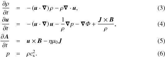 where u the velocity, A is the magnetic potential (B = ∇ × A),
  is the current density, p is the pressure, and cs is the sound speed. The gravitational potential Φ = −GM⋆/r where G is the gravitational constant, M⋆ is the stellar mass, and r is the cylindrical radius. The resistivity is a radial function of position. We use smooth step functions
 ![Mathematical equation: \begin{equation} \eta(r) = \eta_0 - \frac{\eta_0}{2}\left[\tanh\left(\frac{r-r_1}{h_1}\right) -\tanh\left(\frac{r-r_2}{h_2}\right)\right] \label{eq:eta-jump} \end{equation}](/articles/aa/full_html/2015/02/aa24919-14/aa24919-14-eq35.png) (7)in order to mimic the effect of a dead zone. The resistivity passes from η0 to zero over a width h1 centered at an arbitrarily chosen distance r1. The second transition is for buffer purposes, raising the resistivity above the MRI-triggering threshold near the outer boundary of the domain.
(7)in order to mimic the effect of a dead zone. The resistivity passes from η0 to zero over a width h1 centered at an arbitrarily chosen distance r1. The second transition is for buffer purposes, raising the resistivity above the MRI-triggering threshold near the outer boundary of the domain.
We solve the equations with the Pencil code1 which integrates the evolution equations with sixth order spatial derivatives, and a third order Runge-Kutta time integrator. Sixth-order hyper-dissipation terms are added to Eqs. (3)–(5), to provide extra dissipation near the grid scale, explained in Lyra et al. (2008a). They are needed because the high order scheme of the Pencil code has little overall numerical dissipation (McNally et al. 2012).
2.1. Initial conditions
We model a disk similar to Lyra & Mac Low (2012) in cylindrical coordinates (r,φ,z). The disk ranges over r = [0.4, 9.6] r0, φ = [− π,π], and z = [− 0.1, 0.1]. The resolution is [Nr, Nφ, Nz] = [512, 512, 32]. The radial spacing is non-uniform, keeping a constant number of points per radial scale height (H/ Δr = 16), where Δr = Δr(r) is the (local) radial resolution. The vertical direction is unstratified, and the main purpose of its presence is to resolve the MRI.
We use units such that  (8)The density and sound speed are set as radial power-laws
 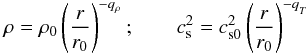 (9)with qρ = 1.5 and qT = 1.0. The reference sound speed is set at cs0 = 0.1, and Gaussian-distributed noise is added to the velocities, cell by cell, at rms equal to 10-3 times the local sound speed. The initial angular velocity profile is corrected by the thermal pressure gradient
  (10)where Ω = Ω0 (r/r0)− q with q = 1.5 is the Keplerian angular velocity.
The magnetic field is set as a net vertical field, with two MRI wavelengths resolved in the vertical range. The constraint λMRI = 2πvAΩ-1 = Lz/ 2 translates into a radially varying field  (11)i.e., a field falling as a 9/4 power-law, with B0 = vA ≈ 1 × 10⁻² in code units. Since the magnetic field is not needed in the resistive inner disk, we bring it smoothly to zero inward of r = 2.5. The dimensionless plasma beta parameter
  ranges from 103 to 104 in the active zone. In this configuration, the MRI grows and saturates quickly in 3 local orbits. We use reflective boundaries, with a buffer zone of width H at each radial border, that drives the quantities to the initial condition on a dynamical timescale.
In the presence of resistivity, the behavior of the MRI is controlled by the magnetic Reynolds number ReM = LvA/η where L is a relevant length scale. Setting L = vA/Ω defines the Elsasser number Λ. Because the MRI exists for arbitrarily large wavelengths (Balbus & Hawley 1991), a more relevant length scale, that controls the excitation of the MRI, is the longest wavelength present in the vertical domain. For stratified disks, this wavelength is L = H. In the unstratified case, it is simply L = Lz. Once this wavelength is in the resistive range, the MRI is quenched (e.g., Pessah 2010; Lyra & Klahr 2011). That defines a “box” Lundquist number,  (12)We set the reference resistivity η0 so that Lu is unity at r1, thus quenching the MRI inward of this radius. This constraint translates into η0 = LzvA = 5 × 10⁻⁴. We place the resistivity jump starting at r1 = 2.5, and vary the transition width h1. For h1 = 0.8, the resistivity jump goes from Lu ≈ 0.1 to 1 from the inner disk to r = 2.5, and thence to Lu ≈ 10 at r ≈ 4. Considering r0 = 10 AU, this corresponds to the physical dead-to-active transition in the outer disk (Dzyurkevich et al. 2013). We fix r2 = 10 and h2 = 0.8 for the second transition.
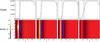 |
Fig. 2 Two-dimensional hydrodynamical alpha-disks, with viscosity transitions (upper panels) equivalent to the resistivity ones, and αν ≈ 0.02 in the “active” zone (the subscript ν underscores that this α corresponds to a Laplacian viscosity, not to turbulent stresses). The lower panels show the density, for snapshots at the same times as in Fig. 1. Only the first ones (h1 = 0.1 and h1 = 0.2) develop the RWI. |
3. Results
We show in Fig. 1 the results of the suite of MHD simulations. The only difference between the models is the width of the transition from the (inner) dead zone to the active zone. From left to right, the transition width h1 is 0.1, 0.2, 0.4, and 0.8. The upper panels show the corresponding resistivity jumps; the dashed vertical lines mark a width of 2H around r = 2.5. For the latter two simulations, the transition in resistivity is significantly wider than 2H.
The middle panels show the density in the midplane, normalized by the initial density. The RWI was excited in all models. The vortex is seen as a non-axisymmetric density enhancement around (but not exactly at) the resistivity transition center at r = 2.5. The white dashed lines correspond to a 2H width centered at the density maximum. That the 2H lines box the structures is evidence that they are indeed vortices (whose size is limited by shocks and therefore approximately 2H, cf., Lyra & Lin 2013). The snapshots are at 100, 100, 122, and 232 orbits.
In the middle panels we show the turbulent alpha values, i.e., the magnetic and kinetic turbulent stresses normalized by the local pressure (Shakura & Sunyaev 1973). We define them, respectively, as  (13)where the angled brackets represent vertical and azimuthal average. The prime represents a fluctuation from a mean, defined as ξ′ = ξ − ⟨ ξ ⟩, where ξ is an arbitrary quantity. As seen in the figure, both stresses level at α ≈ 0.01. The Maxwell stress is well confined to the active zone; the Reynolds stress in the dead zone is roughly an order of magnitude lower than in the active zone.
We show in Fig. 2 the corresponding 2D viscous alpha-disk simulations. The viscosity profile corresponds to that of the resistivity, but with minima and maxima swapped, ![Mathematical equation: \begin{equation} \nu(r) = \frac{\nu_0}{2} \left[\tanh\left( \frac{r-r_1}{h_1}\right) - \tanh\left( \frac{r-r_2}{h_2} \right) \right]\cdot \end{equation}](/articles/aa/full_html/2015/02/aa24919-14/aa24919-14-eq86.png) (14)The values of r1, h1, r2 and h2 are identical to those used in the MHD models. The second jump is not needed in the viscous calculation, but kept for symmetry reasons. The value of ν0 is chosen consistently with the value of α ≈ 0.02 (for the combined kinetic and magnetic stresses) derived from the MHD calculation.
(14)The values of r1, h1, r2 and h2 are identical to those used in the MHD models. The second jump is not needed in the viscous calculation, but kept for symmetry reasons. The value of ν0 is chosen consistently with the value of α ≈ 0.02 (for the combined kinetic and magnetic stresses) derived from the MHD calculation.
The snapshots were taken at the same times. In agreement with previous alpha-disk works on the RWI, but in contrast to the MHD runs shown in Fig. 1, only in the first two simulations, where the viscosity jump is sharper than 2H, was the RWI triggered.
4. Discussion
According to RWI theory, the instability will be triggered if a quantity ℒ, associated with vortensity, has an extremum somewhere in the disk. In the context of locally isothermal disks ℒ is half the inverse of vortensity  (15)where ωz is the vertical vorticity. Amplitude and sharpness of the transition also play a role, although a strict criterion has not been derived. Linear analysis predicts instability if any extremum exists, but empirically, it is found that critical amplitude and sharpness exist for the onset of instability. Li et al. (2000) report that as a rule-of-thumb the instability is triggered when the density varies by 10%−20% over lengths scales comparable to the scale height H; a condition subsequently confirmed in later simulations with different numerical schemes and different resolutions.
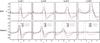 |
Fig. 3 Density bumps at selected snapshots, for the MHD simulations (upper panels) and alpha-disk equivalents (lower panels). The dashed lines bracket 2H around the density maximum of the last snapshot shown (red line). The RWI “rule-of-thumb” of 10−20% variation in density over a width comparable to the scale height is satisfied for the MHD turbulent runs, even for the wide transition model of h1 = 0.8. In the equivalent viscous laminar model the density bumps diffuse over a much larger width, and the RWI is not excited. |
We show in Fig. 3 that this rule-of-thumb is met in the MHD simulations for the transition widths used. The figure shows, for each width used, the density bump in the MHD runs and alpha-disk equivalent, in three different snapshots, labeled in the figure. In the viscous run (lower panels) the smoothness of the resulting density bump is strongly correlated with the width of the viscous jump. The same does not happen for the MHD run, where the density bump is sharp in all cases, and, although the rate of mass accumulation slows down as the resistivity transition widens, the smoothness of the bump is only weakly correlated with the width of the resistivity gradient, remaining sharp in all cases tested. We did not explore further than the transition width h1 = 0.8 because, taking r0 = 10 AU, that width corresponds to a transition over 30 AU, which is the physical value expected for the dead-active transition in the outer disk (Dzyurkevich et al. 2013). The conclusion is that in physical disks, even the smooth outer resistivity transition can excite the RWI.
That even this smooth transition can lead to excitation of the RWI is in principle unexpected. How can the density bump be so sharp? The solution seems to be in the Maxwell stress. Although the resistivity is smooth, the transition in Maxwell stress remains sharp, a feature that is absent in the alpha-disk viscous equivalent. The origin of this behavior is a property of the MRI. The MRI is excited and maintained for Lu > 1, which always constitutes a sharp transition to turbulence. So, in essence, it is a property of turbulent flows. As long as the critical wavelength is not within the resistive range, the MRI will be excited. This is in agreement with the shearing box results of Sano & Stone (2002). The novelty of this work is to show that this non-uniform η − α relationship triggers the RWI even for weak gradients of η. Maxwell stresses drive the gas inwards (away from the pressure maximum), placing it at the transition, at the laminar side. Inviscid, the density bump is slightly blurred by Reynolds stresses, but does not spread viscously as in the alpha-disk case, and thus remains sharp. Because the vortex is in the resistive side of the transition, it does not get destroyed by the magneto-elliptic instability (Mizerski & Bajer 2009; Lyra & Klahr 2011; Mizerski & Lyra 2012).
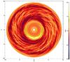 |
Fig. 4 Cartesian projection of the MHD model with h1 = 0.8, with the smooth resistivity jump from r ≈ 1 to r ≈ 4, i.e. roughly 15 scale heights. Although the resistivity jump is smooth, the resulting transition in Maxwell stress is sharp, triggering the Rossby vortex. Notice also the conspicuous spiral pattern propagating into the dead zone. An animation of the simulation is available online. |
We show in Fig. 4 a Cartesian projection of the MHD model with h1 = 0.8. The Rossby vortex is conspicuous as a crescent-shaped overdensity at r ≈ 2. Notice also the spiral pattern in the dead zone. Reminiscent of planet-induced spirals, in this case the spiral is the result of waves propagating inwards, from the turbulence in the active zone.
5. Conclusions
The RWI requires a sharp extremum of potential vorticity. In alpha disks, this bump comes about only at sharp viscosity transitions, sharper than 2H. This, although making the inner active/dead zone transition attractive for the RWI, has hindered the appeal of the outer dead/active zone transition as a RWI location.
Sano & Stone (2002) found that, in shearing boxes, the Maxwell stress increases sharply with Elsasser number in the range below unity. Bringing the result to global disks, we have found that the required sharpness of the viscosity transition for RWI is a feature of alpha disks. We have increased the width of the resistivity transition without finding a RWI cutoff. Resistivity transitions can be as smooth as 30 AU in width in the outer disk and still excite the RWI. This is because once the MRI is excited growth rates can be affected by resistivity, but the resulting amplitude at saturation is only weakly affected by it. As a result, the transition in Maxwell stress remains sharp, driving mass to the dead side of the transition. Once there, without Laplacian viscosity to smooth it, the density bump remains sharp, triggering the RWI as it collects mass.
Our finding has importance for the interpretation of observations of dust asymmetries in transitional disks (van der Marel et al. 2013; Casassus et al. 2013; Isella et al. 2012, 2013; van der Plas et al. 2014), for which the best explanation is a vortex. A vortex can be brought about by RWI in gaps carved by planets (de Val Borro 2007; Lyra et al. 2009b; Lin & Papaloizou 2011a,b; Lin 2012), by convective overstability (Klahr & Hubbard 2014; Lyra 2014), or by RWI at dead zone boundaries (Varniere & Tagger 2006; Lyra et al. 2008b, 2009a). A planetary gap is an exciting possibility (Zhu & Stone 2014), but before an undetected planet is invoked, other alternatives ought to be dealt with. In the case of Oph IRS 48, convective overstability fails to operate, because the disk is supposedly too radiatively efficient; as for dead zone boundaries, the transition in resistivity was thought too smooth to lead to RWI. We have shown that the latter is not a deterrent. RWI in the outer dead/active transition may be the culprit for the vortex of Oph IRS 48.
Notice also the spiral pattern in the dead zone in Fig. 4. Similar spiral patterns have been observed in actual disks (SAO 206462, Muto et al. 2012), and attributed to unseen planets. In our simulation, these are simply spiral density waves that propagate inward, launched by the turbulence in the active zone. The spiral pattern comes about because without turbulent interference, they propagate coherently. A proper comparison to the observations would require the addition of particles in order to study how they are trapped in these spirals, which we leave for future work. At first, we expect the resulting particle concentration to be stronger than the trapping in planetary spirals, that are stationary in the reference frame of the planet and thus only trap the very well-coupled dust (Lyra et al. 2009b). In contrast, these dead zone spirals rotate at the disk’s velocity and hence should be able to capture more loosely coupled particles (Ataiee et al. 2013).
We caution that our models have several limitations. They are unstratified MHD calculations with static Ohmic resistivity profiles. Stratification should have little effect on the linear growth of the RWI, which is essentially 2-dimensional (Umurhan 2010; Meheut et al. 2012a,b; Lin 2012a,b, 2013). However stratification will influence the outcome by setting a physical scale for the resistivity cutoff: in unstratified models the results depend on box size, because the Lundquist number is a function of Lz. In stratified models this artificial parameter is replaced by the density scale height H. Furthermore the saturated RWI may be severely affected by the vertical structure. Lin (2014) finds that Rossby vortices are transient in disks with a higher-viscosity surface layer (Gammie 1996) if the density bump spreads out once the vortex forms. Here the vortex is long-lived only if the accretion viscosity is low throughout the column. However, Lin (2014) also finds that if the viscosity is such as to maintain the density bump, the vortex is sustained despite the layered structure. This latter situation is more similar to our case, where the turbulent stresses bring material to the dead zone edge, strengthening the density bump. Further study of vortex lifetimes in layered surroundings is warranted, especially treating the ambipolar and Hall terms, which can greatly alter the vertical structure of the weakly-ionized annuli in protostellar disks (Wardle 1999; Bai & Stone 2011, 2013; Wardle & Salmeron 2012; Mohanty et al. 2013; Kunz & Lesur 2013; Lesur et al. 2014). The resistivity’s time-dependence has less effect, judging from the results of Faure et al. (2014).
The layered structure of the magnetic activity potentially has a special impact at the dead zone edge, where the stratification can yield a vertically-averaged stress that varies more smoothly with radius than the midplane profile represented in our unstratified calculations. A smoother stress profile would lead to a broader density bump, weakening our conclusion. However, dead zone structure calculations treating the Ohmic and ambipolar terms in prescribed surface density profiles indicate the transition from dead to active zone forms a vertical wall up to ± H (Fig. 4a of Dzyurkevich et al. 2013). Between H and 2H, the boundary bends further from the star, but is set by the ambipolar diffusion, which will weaken as the density bump builds up. Over time, mass is thus likely to accumulate in a narrow range of radii near the position of the dead zone’s edge in the midplane. The feedback between the evolving density distribution and the evolving diffusivities deserves further investigation.
Our results are evidence of the practical importance of developing a detailed picture of the underlying turbulence mechanisms in protoplanetary disks. As demonstrated here, such models can have a critical impact on how observations are understood.
Online material
Movie of Fig. 4 Access Supplementary Material
The code, including improvements done for the present work, is publicly available under a GNU open source license and can be downloaded at http://www.nordita.org/software/pencil-codes.
Acknowledgments
This work was performed in part at the Jet Propulsion Laboratory, under contract with the California Institute of Technology funded by the National Aeronautics and Space Administration (NASA) through the Sagan Fellowship Program executed by the NASA Exoplanet Science Institute. The research leading to these results has received funding from the People Programme (Marie Curie Actions) of the European Union’s Seventh Framework Programme (FP7/2007-2013) under REA grant agreement 327995. We acknowledge discussions with Min-Kai Lin and Zhaohuan Zhu.
References
- Ataiee, S., Pinilla, P., Zsom, A., et al. 2013, A&A, 553, A3 [NASA ADS] [CrossRef] [EDP Sciences] [Google Scholar]
- Bai, X.-N., & Stone, J. M. 2011, ApJ, 736, 144 [NASA ADS] [CrossRef] [Google Scholar]
- Bai, X.-N., & Stone, J. M. 2013, ApJ, 769, 76 [NASA ADS] [CrossRef] [Google Scholar]
- Balbus, S. A., & Hawley, J. F. 1991, ApJ, 376, 214 [NASA ADS] [CrossRef] [Google Scholar]
- Brandenburg, A., & Dobler, W. 2002, Comput. Phys. Common., 147, 471 [Google Scholar]
- Casassus, S., van der Plas, G., Perez, S., et al. 2013, Nature, 493, 191 [NASA ADS] [CrossRef] [Google Scholar]
- Dzyurkevich, N., Turner, N. J., Henning, T., & Kley, W. 2013, ApJ, 765, 114 [NASA ADS] [CrossRef] [Google Scholar]
- Faure, J., Fromang, S., & Latter, H. 2014, A&A, 564, A22 [NASA ADS] [CrossRef] [EDP Sciences] [Google Scholar]
- Gammie, C. F. 1996, ApJ, 457, 355 [NASA ADS] [CrossRef] [Google Scholar]
- Hawley, J. F. 1987, MNRAS, 225, 677 [NASA ADS] [CrossRef] [Google Scholar]
- Isella, A., Pérez, L. M., & Carpenter, J. M. 2012, ApJ, 747, 136 [NASA ADS] [CrossRef] [Google Scholar]
- Isella, A., Pérez, L. M., Carpenter, J. M., et al. 2013, ApJ, 775, 30 [NASA ADS] [CrossRef] [MathSciNet] [Google Scholar]
- Klahr, H., & Hubbard, A. 2014, ApJ, 788, 21 [NASA ADS] [CrossRef] [Google Scholar]
- Kerswell, R. R. 2002, AnRFM, 34, 83 [Google Scholar]
- Kunz, M. W., & Lesur, G. 2013, MNRAS, 434, 2295 [NASA ADS] [CrossRef] [Google Scholar]
- Lesur, G., & Papaloizou, J. C. B. 2009, A&A, 498, 1 [NASA ADS] [CrossRef] [EDP Sciences] [Google Scholar]
- Lesur, G., & Papaloizou, J. C. B. 2010, A&A, 513, A60 [NASA ADS] [CrossRef] [EDP Sciences] [Google Scholar]
- Lesur, G., Kunz, M. W., & Fromang, S. 2014, A&A, 566, A56 [NASA ADS] [CrossRef] [EDP Sciences] [Google Scholar]
- Li, H., Finn, J. M., Lovelace, R. V. E., & Colgate, S. A. 2000, ApJ, 533, 1023 [NASA ADS] [CrossRef] [Google Scholar]
- Li, H., Colgate, S. A., Wendroff, B., & Liska, R. 2001, ApJ, 551, 874 [NASA ADS] [CrossRef] [Google Scholar]
- Lin, M.-K., & Papaloizou, J. C. B. 2011a, MNRAS, 415, 1426 [NASA ADS] [CrossRef] [Google Scholar]
- Lin, M.-K., & Papaloizou, J. C. B. 2011b, MNRAS, 415, 1445 [NASA ADS] [CrossRef] [Google Scholar]
- Lin, M.-K. 2012a, ApJ, 754, 21 [Google Scholar]
- Lin, M.-K. 2012b, MNRAS, 426, 3211 [NASA ADS] [CrossRef] [Google Scholar]
- Lin, M.-K. 2013, ApJ, 765, 84 [NASA ADS] [CrossRef] [Google Scholar]
- Lin, M.-K. 2014, MNRAS, 437, 575 [NASA ADS] [CrossRef] [Google Scholar]
- Lovelace, R. V. E., & Hohlfeld, R. G. 1978, ApJ, 221, 51 [NASA ADS] [CrossRef] [Google Scholar]
- Lovelace, R. V. E., Li, H., Colgate, S. A., & Nelson, A. F. 1999, ApJ, 513, 805 [NASA ADS] [CrossRef] [Google Scholar]
- Lyra, W. 2014, ApJ, 789, 77 [NASA ADS] [CrossRef] [Google Scholar]
- Lyra, W., & Klahr, H. 2011, A&A, 527, A138 [NASA ADS] [CrossRef] [EDP Sciences] [Google Scholar]
- Lyra, W., & Lin, M.-K. 2013, ApJ, 775, 17 [NASA ADS] [CrossRef] [Google Scholar]
- Lyra, W., & Mac Low, M.-M. 2012, ApJ, 756, 62 [NASA ADS] [CrossRef] [Google Scholar]
- Lyra, W., Johansen, A., Klahr, H., & Piskunov, N. 2008a, A&A, 479, 883 [NASA ADS] [CrossRef] [EDP Sciences] [Google Scholar]
- Lyra, W., Johansen, A., Klahr, H., & Piskunov, N. 2008b, A&A, 491, L41 [NASA ADS] [CrossRef] [EDP Sciences] [Google Scholar]
- Lyra, W., Johansen, A., Zsom, A., Klahr, H., & Piskunov, N. 2009a, A&A, 497, 869 [NASA ADS] [CrossRef] [EDP Sciences] [Google Scholar]
- Lyra, W., Johansen, A., Klahr, H., & Piskunov, N. 2009b, A&A, 493, 1125 [NASA ADS] [CrossRef] [EDP Sciences] [Google Scholar]
- McNally, C. P., Lyra, W., & Passy, J.-C. 2012, ApJS, 201, 18 [NASA ADS] [CrossRef] [Google Scholar]
- Méheut, H., Casse, F., Varnière, P., & Tagger, M. 2010, A&A, 516, A31 [NASA ADS] [CrossRef] [EDP Sciences] [Google Scholar]
- Méheut, H., Cong, Y., & Lai, D. 2012a, MNRAS, 422, 2399 [NASA ADS] [CrossRef] [Google Scholar]
- Méheut, H., Keppens, R., Casse, F., & Benz, W. 2012b, A&A, 542, A9 [Google Scholar]
- Mizerski, K. A., & Bajer, K. 2009, J. Fluid Mech., 632, 401 [NASA ADS] [CrossRef] [Google Scholar]
- Mizerski, K. A., & Lyra, W. 2012, J. Fluid Mech., 698, 358 [NASA ADS] [CrossRef] [Google Scholar]
- Mohanty, S., Ercolano, B., & Turner, N. J. 2013, ApJ, 764, 65 [NASA ADS] [CrossRef] [Google Scholar]
- Muto, T., Grady, C. A., Hashimoto, J., et al. 2012, ApJ, 748, L22 [NASA ADS] [CrossRef] [Google Scholar]
- Papaloizou, J. C. B., & Pringle, J. E. 1984, MNRAS, 208, 721 [NASA ADS] [CrossRef] [Google Scholar]
- Papaloizou, J. C. B., & Pringle, J. E. 1985, MNRAS, 213, 799 [NASA ADS] [Google Scholar]
- Pessah, M. 2010, ApJ, 716, 1012 [NASA ADS] [CrossRef] [Google Scholar]
- Regály, Z., Juhász, A., Sándor, Z., & Dullemond, C. P. 2012, MNRAS, 419, 1701 [NASA ADS] [CrossRef] [Google Scholar]
- Sano, T., & Stone, J. M. 2002, ApJ, 577, 534 [NASA ADS] [CrossRef] [Google Scholar]
- Shakura, N. I., & Sunyaev, R. A. 1973, A&A, 24, 337 [NASA ADS] [Google Scholar]
- Tagger, M. 2001, A&A, 380, 750 [NASA ADS] [CrossRef] [EDP Sciences] [Google Scholar]
- Toomre, A. 1981, What amplifies the spirals. In The Structure and Evolution of Normal Galaxies, Proc. of the Advanced Study Institute, Cambridge, England (Cambridge, New York: Cambridge University Press), 111 [Google Scholar]
- van der Marel, N., van Dishoeck, E. F., Bruderer, S., et al. 2013, Science, 340, 1199 [NASA ADS] [CrossRef] [PubMed] [Google Scholar]
- van der Plas, G., Casassus, S., Mnard, F., et al. 2014, ApJ, 792, 25 [NASA ADS] [CrossRef] [Google Scholar]
- Umurhan, O. M. 2010, A&A, 521, A25 [NASA ADS] [CrossRef] [EDP Sciences] [Google Scholar]
- Varnière, P., & Tagger, M. 2006, A&A, 446, 13 [Google Scholar]
- Wardle, M. 1999, MNRAS, 307, 849 [NASA ADS] [CrossRef] [Google Scholar]
- Wardle, M., & Salmeron, R. 2012, MNRAS, 422, 2737 [NASA ADS] [CrossRef] [Google Scholar]
- Zhu, Z., & Stone, J. M. 2014, ApJ, 795, 53 [NASA ADS] [CrossRef] [Google Scholar]
All Figures
|
Fig. 1 Suite of MHD simulations. From left to right, the transition width is h1 = 0.1, 0.2, 0.4 and 0.8. The resulting resistivity profiles are shown in the upper panels. The dashed vertical lines correspond to 2H around the jump center at r = 2.5. The model with h1 = 0.8 corresponds to a smooth jump from r ≈ 1 to r ≈ 4, i.e., over ≈15 scale heights. Although at different times, all models develop a sharp density bump that goes unstable to the RWI, producing a Rossby vortex (middle panels). The panels, from left to right, correspond to density snapshots at 100, 100, 122, and 232T0, where T0 is the orbital period at r = 1. The dashed vertical lines correspond to 2H around the density maximum. The reason for RWI excitation in these cases is because even though the resistivity jump is smooth, the transition in Maxwell stress remains sharp (lower panels). The transition in Reynolds stress is somewhat smoother, but turbulent stresses do not blur gradients in the same way Laplacian viscosity does, and the density bump remains RWI-unstable. |
| In the text | |
|
Fig. 2 Two-dimensional hydrodynamical alpha-disks, with viscosity transitions (upper panels) equivalent to the resistivity ones, and αν ≈ 0.02 in the “active” zone (the subscript ν underscores that this α corresponds to a Laplacian viscosity, not to turbulent stresses). The lower panels show the density, for snapshots at the same times as in Fig. 1. Only the first ones (h1 = 0.1 and h1 = 0.2) develop the RWI. |
| In the text | |
|
Fig. 3 Density bumps at selected snapshots, for the MHD simulations (upper panels) and alpha-disk equivalents (lower panels). The dashed lines bracket 2H around the density maximum of the last snapshot shown (red line). The RWI “rule-of-thumb” of 10−20% variation in density over a width comparable to the scale height is satisfied for the MHD turbulent runs, even for the wide transition model of h1 = 0.8. In the equivalent viscous laminar model the density bumps diffuse over a much larger width, and the RWI is not excited. |
| In the text | |
|
Fig. 4 Cartesian projection of the MHD model with h1 = 0.8, with the smooth resistivity jump from r ≈ 1 to r ≈ 4, i.e. roughly 15 scale heights. Although the resistivity jump is smooth, the resulting transition in Maxwell stress is sharp, triggering the Rossby vortex. Notice also the conspicuous spiral pattern propagating into the dead zone. An animation of the simulation is available online. |
| In the text | |
Current usage metrics show cumulative count of Article Views (full-text article views including HTML views, PDF and ePub downloads, according to the available data) and Abstracts Views on Vision4Press platform.
Data correspond to usage on the plateform after 2015. The current usage metrics is available 48-96 hours after online publication and is updated daily on week days.
Initial download of the metrics may take a while.