| Issue |
A&A
Volume 574, February 2015
|
|
|---|---|---|
| Article Number | A8 | |
| Number of page(s) | 14 | |
| Section | Interstellar and circumstellar matter | |
| DOI | https://doi.org/10.1051/0004-6361/201424859 | |
| Published online | 16 January 2015 | |
Photometry of variable dust-enshrouded stars
Supernovae Ia
Max-Planck-Institut für Radiastronomie, Auf dem Hügel 69, 53121 Bonn, Germany
e-mail: This email address is being protected from spambots. You need JavaScript enabled to view it.
Received: 26 August 2014
Accepted: 17 October 2014
Abstract
We study the time evolution of the spectral energy distribution (SED) of a transient star surrounded by a spatially unresolved spherical dust envelope. We perform radiative transfer calculations following the Monte Carlo method of Bjorkman & Wood (2001, ApJ, 554, 615) which we extend to include time variability. In a preparatory step, we compute the SED of sources whose intrinsic light curve is a step function. Although the stellar spectrum is constant while the star is switched on, the SED, the extinction curve and the colors are variable. In a second step, we model dust-embedded, distant and therefore spatially unresoved supernovae Ia because of the profound cosmological consequences of their photometric data. As before, the colors, the extinction curve and the SED develop in time. The peak bolometric luminosity is much reduced compared to an unreddend SN. The maximum brightness at wavelengths where grains do not radiate (λ< 2 μm) is also substantially reduced relative to a non-variable star of the same luminosity. The light curves in optical bands are broadened and the time of maximum emission delayed, the extinction curves vary with time. All this is caused by the stochastic travel times of interacting photons. The dust temperature in the dust shell is remarkably constant. In the SED, the emission changes from mainly optical to predominantly mid IR. Changing the scattering properties of dust, without changing its extinction coefficient can lead to an underestimate of the supernova peak brightness.
Key words: supernovae: general / radiative transfer / dust, extinction
© ESO, 2015
1. Introduction
The spectral energy distribution (SED) of all more interesting dusty sources, like star forming regions, protostars or mass-loss stars eventually changes, but the changes are slow so that when modelling the transfer of radiation, it is not necessary that the underlying equations contain the time explicitly. The brightness variation of supernovae, however, is rapid with a timescale of ~10 days and it is not excluded that they sometimes explode in a local dusty environment. In such cases, the time variation of the luminosity would have to be incorporated into the SED models. Because of the frequent and seemingly strange behavior of the dust in (extragalactic) supernovae, exemplified by very low values of RV unheard of in the Milky Way, a number of studies have been conducted to elucidate the role of scattering in the light curves. Besides the pioneering work by Chevalier (1986), we mention, in a not complete list, the fruitful papers of Wang (2005), Goobar (2008), Nobili & Goobar (2008), Fischera & Schmidt (2009) and Amanullah & Goobar (2011). The recent supernova 2014J of type Ia in M 82, whose extinction and polarimetry also point towards very unsual dust properties (Amanullah et al. 2014; Foley et al. 2014; Patat et al. 2014), is another stimulus to continue the work.
2. Photometry of dusty sources
We recall the basic definitions used in photometry and extend them, first, to enshrouded and then to variable sources.
2.1. Case A: scattered photons are not detected
Usually in stellar observations, none of the photons that have been scattered are detected. If τλ is the extinction optical depth towards the source at wavelength λ, the light is weakened as a result of absorption and scattering by the factor e−τλ. If V denotes the visual band at 0.55 μm and Kλ the dust extinction coefficient, the wavelength dependence of extinction is given by τλ/τV = Kλ/KV, where Kλ is the sum of absorption and scattering coefficient,  . Because the optical depth is not a directly observable quantity, one usually uses instead of τλ/τV the extinction curve
 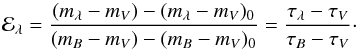 (1)ℰλ and τλ/τV contain the same information. They are both independent of the dust column density, it is irrelevant whether light is removed by absorption or scattering, and neither the albedo
  nor the phase function fλ(θ) (θ is the scattering angle) enter explicitly. In Eq. (1), (mλ − mλ′) is the observed source color and (mλ − mλ′)0 the color of an unreddened comparison star of exactly the same spectral shape. We reserve calligraphic letters (ℰλ,ℛV) for quantities that depend only on Kλ/KV.
2.2. Case B: scattered photons are detected
Alternatively, when the source is dust-enshrouded and the spatial resolution does not allow to separate it from its circumstellar environment, scattered photons may reach the observer. This is generally so for extragalactic stars, but often also in the study of galactic protostellar objects.
If Fobs is the observed flux and Fnd the flux one would detect if there were no dust, we define the effective optical depth τeff by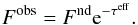 (2)We drop the index λ when the wavelength dependence is obvious. In observations with a pencil beam, i.e., an infinitely small aperture, the effective and extinction optical depth are equal, τeff = τ. Otherwise τeff can only be smaller than τ, it may even be negative. The effective extinction is discussed and examples are given in Krügel (2009). For instance, if there were only scattering and absorption neglible, a star with a dust shell would not be attenuated at all because no photons are destroyed, whereas looked at with a pencil beam, the source would be weakened by the factor exp( − τsca), τsca being the scattering optical depth towards the star.
To derive the reddening law of a dust enshrouded star, one proceeds observationally as in Eq. (1), but the resulting function is now the effective extinction curve 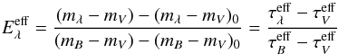 (3)where τ has been substituted by τeff. Even for fixed dust properties, there is no universal extinction curve for dust embedded sources. Instead,
  depends on τV (or any other τλ) and the geometry. Likewise, the ratio of total over selective extinction,
 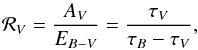 (4)where AV is the attenuation in magnitudes at V and
  (5)the color excess, is replaced by
 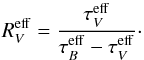 (6)To determine ℛV (or
  ) observationally, firstly, the photometry has to extend to long wavelengths, which seems strange because ℛV is defined by the ratio of the extinction coefficients at B and V only. But the definition of a quantity and its observational derivation are two different matters. Secondly, one needs an unreddened reference star. As this is not around when a SN explodes, one needs a surrogate (template) and trust it.
There is a lot of arbitrariness, or historical burden, in the choice of ℛV, a pair of other bands may sometimes be more suited. The importance of ℛV stems from the fact that it is used to deredden a star to find its unanttenuated brightness.
 is always smaller than ℛV, which one would get from pencil beam observations. This behavior, already noted by Wang (2005) and Goobar (2008), can be understood and almost quantitatively extracted from Fig. 7 in Krügel (2009). According to it, for τ< 1 (single scattering), τ ∝ τeff and therefore
  . However, when τ> 1, the effective extinction τeff rises more strongly than τ (if the albedo ω stays constant). Therefore,
  will be greater than τB/τV, because τB>τV, and thus
  .
.
If the dust distribution around the star is known one can determine τeff theoretically from a radiative transfer calculation. For a homogeneous spherical distribution as in Fig. 2, τeff depends only on the ratio R2/R1 and τ. As  or ℰλ are only meaningful at wavelengths where the dust does not radiate, one has, when computing τeff for a model cloud after Eq. (2), either to neglect the dust emission or set the source luminosity to a very low value; the outcome for τeff is in both cases the same.
2.3. Dust enshrouded variable sources
The previous definitions for  and refer to a stationary source. If it is variable, the extinction curve will vary too, because the average travel time of the scattered photons depends on wavelength. In this paper, we only consider the case where the absolute luminosity of the star changes, its colors (i.e., the shape of its spectrum) stay constant. We denote the time-variable extinction curve by Eλ(t). It follows from
 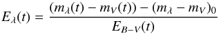 (7)where the color excess
  (8)is now also time-variable, as well as
 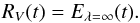 (9)To define an effective optical depth for a variable source and assign a simple physical meaning to it in terms of emitted over detected photons is not possible any more because one would have to specify the moments of emission and detection.
Besides the usual extinction curve, ℰλ of Eq. (1), where the obscuring dust is far from the star and which directly reflects optical dust properties, there are thus two others. First, the effective extinction curve, of Eq. (3), when the dust is circumstellar. It depends on the way the dust is distributed. Second, the extinction curve Eλ(t) of Eq. (7) of a variable source with circumstellar dust.
In the most general case, the star changes also its colors. Then (mλ − mV)0 in Eq. (7) depends also on time and for each moment of observation one needs the appropriate unreddened reference star. This is, strictly speaking, the case for SN Ia, but in our first attempt of analyzing their photometry we assume constant SN colors.
When the obscuring dust is far away from the star, or in pencil beam observations, one will derive ℰλ under any kind of stellar variability because all photons have the same flight time.
The effective extinction curve  no longer yields the dust extinction coefficient ratio Kλ/KV, but one can still use it to deredden a star. Analogous to AV = EB − V ℛV, one can employ to correct for the attenuation by dust and find the true stellar luminosity. The time-variable extinction curve Eλ(t) of Eq. (7), on the other hand, does not tell us anything at all about the intrinsic stellar luminosity, unless its variations are small or we know everything about the time-dependence of the stellar luminosity and the spatial distribution of dust.
3. Model parameters
3.1. The dust model
We assume throughout standard Milky Way dust because its properties are best known and to demonstrate that the basic results of this paper do not require any particular kind of dust. The optical properties of standard dust are, at wavelengths λ ≲ 8 μm, defined by the standard extinction curve (with ℛV = 3.1 equivalent to KB/KV = 1.324) and, adding scattering data, by the dust albedo ωλ and the phase function fλ(θ). The latter two quantities cannot be determined independently one of the other and have considerable error bars. The asymmetry factor gλ is an extract from fλ(θ) characterizing the scattering pattern by one number. We take gλ from Fig. 1a and then, for numerical ease, assume for fλ(θ) a Henyey-Grenstein phase function (it turns out that this particular choice hardly matters). Our underlying data for ωλ,gλ and ℰλ are displayed in Fig. 1.
Without modeling dust radiation, this data set would suffice. To calculate the dust emission, one must a) extend Kλ to longer wavelengths (gλ and ωλ are there close to zero) and b) use various kinds of grains because they will have at the same spot different temperatures and the mix cannot be well approximated by one kind with one temperature.
We assume that Kλ of the dust mixture has at λ> 8 μm the shape of the curve labeled tot in Fig. 10.7 of Krügel (2006) (similar plots by other authors make little difference). The absolute values of Kλ are not needed. The curve results from Mie calculations of spheres composed of silicate (Si), amorphous carbon (aC) and graphite (gr). They have mass fractions fSi = 62%,faC = 27%,fgr = 11%, particle radii aSi = 0.026...0.23 μm, aaC = 0.015...0.23 μm, agr ~ 0.01 μm (MRN size distribution), and optical constants from Weingartner & Draine (2001), Zubko et al. (1996) and Laor & Draine (1993), repsectively.
Although the Kλ,ωλ,gλ from the Mie calculations are not used at short wavelengths, they fit the curves in Fig. 1 very well for λ-1< 6 μm-1, less well, but still tolerably, for λ-1> 6 μm-1. Our data for λ< 8 μm from Fig. 1 and those for λ> 8 μm from Mie theory are therefore internally consistent.
 |
Fig. 1 a) Abedo ω (blue squares) and asymmetry factor, g, (green triangles) for standard dust defined in Sect. 3.1; it is used in all models of this paper. Points mark frequently used wavelengths, like UBVRI ...b) Standard dust produces in pencil beam observations the standard extinction curve ℰλ (red triangles). The black squares display the effective extinction curve assuming a Henyey-Greenstein phase function towards an unresolved shell source (see Fig. 2) with τV = 2 and other parameters as described in Sect. 5.2.1. |
3.2. The intrinsic supernova luminosity
We assume the bolometric luminosity (which means integrated over all wavelengths) of the SN, L∗(t), to vary during its evolution like the analytic function 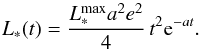 (10)It starts at L(0) = 0, reaches its maximum
  at tmax = 2 /a, drops in the first 15 days after maximum by about Δ15 = 1.13 mag. Equation (10) approximates the average B band light curve of low-redshift SN Ia quite well (Fig. 12b in Frieman et al. 2008) if we put tmax = 11 days. The bolometric luminosity at maximum is set to
  .
.
We further assume that the exploding star is always a blackbody of 10 000 K. All spectral luminosities, L∗ ,λ(t), have therefore the same time dependence as L∗(t). Around maximum, this is in line with the customarily adopted intrinsic colors (e.g., (B − V)0 = 0.05 ± 0.012, Phillips et al. 1999; (B − V)0 = −0.012 ± 0.051, Parodi et al. 2000), but at later times it is a great simplification because the B − V color (Fig. 1 of Phillips et al. 1999), the light curves in other bands (Fig. 1 in Goobar & Leibundgut 2011) as well as the whole spectrum are known to evolve (Hsiao 2007).
3.3. Dust evaporation radius
The evaporation radius Rev of a certain dust component of evaporation temperature Tev and absorption coefficient  follows for a stationary star of luminosity L∗ ,λ from
  (11)With L∗ ,max = 3 × 10⁹L⊙ and Tev = 1500 K, one finds that even small (~100 Å) grains of amorphous carbon or silicate survive at distances greater than 1.5 × 1017 cm. We therefore put the inner radius R1 = 1.5 × 1017 cm.
This is, however, not really correct for a variable star with a light curve of a SN Ia sitting in an initially homogeneous medium. In this case, Rev moves out as the SN luminosity rises. As the computations show, it reaches its maximum radius of about 8 × 1016 cm (instead of 1.5 × 1017 cm) after some 35 days, long after the SN maximum. At SN maximum, light has only traveled to r ~ 3 × 1016 cm. Whether Rev recedes later depends on whether new dust can form, which is unlikely. It is easy to incorporate the time-dependence of Rev into the radiative transfer program. One just has to set the density in a shell where the grain temperature exceeds Tev to zero (but not the photon density, see Sect. 4.2). So our assumption of R1 = 1.5 × 1017 cm is crude, but it has neglegible consequences in our models. For a centrally peaked dust density distribution there could be some differences.
4. Radiative transfer
4.1. The Monte Carlo method
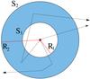 |
Fig. 2 Sketch of a spherical dust envelope around a SN and three possible photon flight paths. Their direction changes after an absorption or scattering event. The inner and outer radii and surfaces of the envelope are R1,R2, and S1,S2, respectively. R1 is equal to the evaporation radius Rev. |
Photons from the star traverse a dust-free zone of radius R1 and enter a spherical envelope of outer radius R2 of dust density ρ(r) (see Fig. 2). In our models, ρ(r) = const. We track their flight paths applying the Monte Carlo strategy of Bjorkman & Wood (2001). It has the great advantage of not requiring iteration and we briefly outline its essence.
-
Photons are binned into packets of equal energyε, those of one packet have the same frequency νj. If one uses N packets, ε = L/N. At each frequency νj, with j = 1,...,mγ, the star releases n packets, therefore N = nmγ. The νj are determined from
 (12)
(12) -
The cloud is partitioned into Nv cells of mass mk,k = 1,2,...,Nv. In our case, the cells are concentric spherical shells. The cells absorb, scatter and emit radiation only in quanta of energy ε; the density, dust composition and grain temperatures are uniform within a cell.
-
A packet at frequency νj interacts along a path of extinction optical depth τj with the dust if τj ≥ − log (z), where z ∈ [0,1] is a random number. The probability for scattering is equal to the albedo,
 , for absorption it is 1 − Aν. When scattered, the packet changes only direction as prescribed by the phase function. When the packet is absorbed, it is isotropically reemitted at νm, which is the smallest frequency for which
 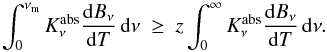 (13)If a cell has already absorbed k ≥ 1 photons, the Planck function in Eq. (13) is evaluated at the cell temperature Tk which follows from the radiative energy balance
  (14)
(14)
4.2. The Bjorkman & Wood method for variable sources
The Bjorkman & Wood method was devised for stationary objects. We extend it to variable sources. If for all cells the number and composition of incoming and outgoing photons changes only weakly over a time interval Δt, one may replace the continuous evolution of the star and the cloud by a sequence of quasi-stationary steps of length Δt. During such an interval, photons diffuse from one cell (or the star) to another, or they only change position within one cell.
To compute the propagation of the photons, we proceed in the following way.
-
The time is segmented into intervalsIi = [ti,ti + 1] ,i = 1,2,... At t = ti, the star emits Ni photons, nij at frequency j with j = 1,...,mγ. The stellar bolometric luminosity, L∗(ti), during Ii is constant and given by L∗(ti) = Niε, where
-
Let L∗ ,ν(t) be the spectral luminosity of the star,
 . At time step i, L∗ ,ν(ti) is controlled via nij. The total number of stellar photons (bold face letter N) released up to the time ti is
-
The photons are numbered in sequence of their emission from ℓ = 1,...,Ni. To each photon ℓ ∈ [1,Ni], we attach five parameters: 1) its age tℓ, counted from the moment it is emitted from the star; 2) its radius rℓ equal to the distance from star; 3) its direction given by the cosine μℓ of the angle with the radius vector; 4) its frequency νℓ (which usually changes upon absorption); 5) a presence flag pℓ equal to 1 while the photon is still in the cloud and 0 otherwise.
-
At the beginning of each time interval Ii, we set k in Eq. (14) in all cells to zero. We then follow the paths of all photons ℓ ∈ [1,Ni] with pℓ = 1 over the interval Ii and keep record of the above five parameters.
4.3. Technical remarks
-
1.
We typically use 500 radial grid points andmγ = 3000 frequencies (see Eq. (12)).
-
2.
We conclude from numerical experiments that for our SN Ia models a time step Δt of one day is sufficiently short and support this conclusion by pointing out the analogy to the Courant-Friedrichs stability criterion for explicit difference schemes in gas dynamics which requires that the time step multiplied by the sound speed, vs, should not be larger than the cell size. Our Monte Carlo scheme is explicit, c is the information propagation velocity, so if one replaces vs by c, the criterion would be fulfilled.
-
3.
As the star is much hotter than the cloud, the frequency set, νj, from Eq. (12) is not fine enough with regard to the emission of dust. One must therefore add interpolated frequencies in the near and mid infrared and extrapolate to frequencies in the FIR. The energy quantum, ε, is, of course, for both sets at all frequencies the same.
-
4.
To save computer storage, we renumber the packets after every ~50 time steps eliminating those that have already left the cloud.
-
5.
We use two dust species: silicate and amorphous carbon grains. At the same spot, they have different temperatures. One may easily include more species.
-
6.
Packets leaving the cloud are recorded and binned according to time and frequency. If one wishes to obtain SEDs under certain viewing angles or construct maps, one must also store the flight direction of the photons and the position from where they left the surface.
4.4. Display of light curves
Consider a variable star of spectral luminosity L∗ ,λ(t) in a cloud, as in Fig. 2, of optical thickness τλ. To demonstrate the effect on the light curve produced by the stellar variability alone, we compare the luminosity Lcl,λ(t) emanating from the cloud around the variable star with the luminosity  from a stationary star of the same L∗ ,λ(t) and in the same environment;
  is the effective extinction defined in Eq. (2).
We restrict the discussion to optical wavelengths where dust emission is negligible. This is always the case in the filters UBVI at λ = 0.36, 0.44, 0.55, 0.9 μm and, if the stellar luminosity or the dust evaporation temperature are low, also at J or K (1.25 and 2.2 μm).
Let  be the maximum of L∗ ,λ(t) (with respect to time) and likewise the maximum of the bolometric luminosity L∗(t). Our SN models have a time-constant spectral shape, so
 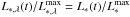 . We plot the light curves in the form
 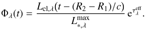 (15)The clock on the right side of in Eq. (15) is set back by (R2 − R1) /c, equal to the flight time of a non-interacting photon through the shell (Fig. 2), to synchronize the stellar flux at S1 with the flux emerging from the cloud at S2.
Without a dust envelope, Φλ(t) would be identical to  , the normalized bolometric stellar light curve. With an envelope and if the velocity of light were infinite, Φλ(t) would also equal
  . But the velocity of light is finite. The difference between Φλ(t) and the normalized stellar bolometric light curve is caused by the delay in the arrival times of scattered photons. The effect of dust absorption is included in Φλ(t).
The flux  detected by an observer, expressed in units of the maximum stellar flux, is
 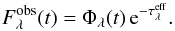 (16)
(16)
5. Results
5.1. The stellar light curve L∗(t) is a step function
Before discussing supernova models, we treat in a preparatory step two light curves in the form of step functions. In both cases, the star is a 104 K blackbody, its luminosity is low enough to suppress dust emission at λ< 10 μm, and the extinction visual optical depth τV equals 1 or 2. The τλ at other wavelengths, as well as gλ and ωλ, follow from Fig. 1.
5.1.1. Model A: the star is switched on and its luminosity stays constant
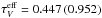
The star lights up at t = 0 and has a constant luminosity LA afterwards: L∗(t) = 0 for t< 0 and L∗(t) = LA = 3 × 10³L⊙ for t> 0. The envelope radii (Fig. 2) are R1 = 6 × 1016 cm and R2 = 0.1 pc = 3.086 × 1017 cm. For the effective optical depths of Eq. (2), one finds  (for τV = 1) and 0.991 (τV = 2), they are thus considerably smaller than the extinction optical depth τV, and the effective ratio of total over selective extinction, equals only 1.854 and 1.845, respectively.
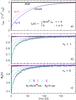 |
Fig. 3 Model A. a) The total luminosity of the unobscured star (thick black line) and the envelope for τV = 1 and 2. b) and c) Light curves Φλ(t) as defined by Eq. (15) in various Johnson filters. Here and in the following figures, the bands can be identified by their colors. The black horizontal line is the normalized light curve of the star. For further parameters, see text. |
Figure 3a shows the bolometric luminosity of the star and the cloud, L∗(t) and Lcl(t), offset in time by (R2 − R1) /c. When the cloud becomes visible at t = 0, it starts with a value much smaller (~8 times for τV = 2) than LA because all scattered or absorbed and then reemitted photons arrive with a delay at the outer surface S2 compared to those that travel on a straight line. The bolometric cloud luminosity Lcl(t) asymptotically approaches L∗ with a “relaxation time” (R2 − R1) /c ≃ 96 days.
Figure 3b (τV = 1) and Fig. 3c (τV = 2) display the light curves Φλ(t) of Eq. (15) for the bands UVIJK, which are all free from dust emission. Their shape is similar to the bolometric light curve Lcl(t), but the relaxation time is shorter.
As Φλ(t) describes the flux reduction due only to prolonged photon travel times, to obtain the full reduction relative to an unobscured stationary star, fred, one still has to multiply by e−τλeff. In the U filter, the effective extinction  for τV = 2. The intensity of the first light from the cloud (near t = 0), compared to an unobscured star, is therefore reduced by the factor
 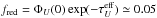 .
.
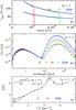 |
Fig. 4 Model A, τV = 1. a) Dust temperatures in the cloud 20, 70 and 150 day after the first photons enter the envelope. Upper lines: amorphous carbon, lower lines: silicate grains. b) The SED 5, 10, 20, 40 and 150 days after the cloud becomes visible. c) The extinction curve 1, 20 and 150 days after the cloud becomes visible. The dotted line marks the effective, the dashed one the standard extinction curve. |
Figure 4 shows at various times the run of the dust temperature, Tdust(r) for the silicate and amorphous carbon grains, the SED and the extinction curve Eλ(t) after Eq. (7). The pictures refer to a visual extinction optical depth of τV = 1.
In Fig. 4a, the time is counted from the moment photons enter the shell, 96 days later they reach the cloud edge. The blue lines at t = 150 days are, within the numerical errors, identical to those of the stationary source (not shown). When the cloud is not yet visible (for t< 96 days), the temperature profiles are also quite close to the stationary case, of course, only up to distances to which photons have traveled.
The SEDs are plotted between 5 and 150 days after visibility and for a source distance of D = 10 Mpc (Fig. 4b). They increase moderately with time at short wavelengths (up to a factor of two), but strongly in the far infrared (factor 20) which is all dust emission. After 150 days, the SED is identical to that of a stationary source.
When the first light emerges from the envelope, the extinction curve Eλ(t) (Fig. 4c) is equal to the normal extinction curve ℰλ of Eq. (1) because scattered photons, which would distort it, can only reach the observer with some delay. For t → ∞, Eλ(t) approaches the effective extinction curve of Eq. (3), appropriate for a stationary dust-enveloped star. The relaxation time is again roughly 100 days.
The results for τV = 2 are very similar to those in Fig. 4, we therefore do not show them. Only the dust temperatures are a bit lower (the cloud has twice the mass, but it has not absorbed twice as much radiative energy), the optical fluxes in the SED are a little smaller (they scale with exp(−τλ)), and the FIR fluxes are enhanced.
5.1.2. Model B: the star is switched on and off
The only difference with respect to Model A is that the star is switched off again after 100 days, which is about equal to the photon travel time through the shell. This mimics, in a zeroth approximation, a supernova: light goes on and off.
As in Model A, the bolometric cloud luminosity, Lcl(t), is initially, near t = 0, about three (τV = 1) or eight (τV = 2) times weaker than the stellar luminosity LA (Fig. 5a). It steadily rises to about ~90% of the full value, abruptly slumps after 100 days when the supply of non-interacting stellar photons has dried out and only scattered or reemitted photons remain in the cloud, and then gradually declines as the photons diffuse out.
The light curves Φλ(t) in Figs. 5b and c (for τV = 1 and 2) exhibit a similar increase in the first 100 days and then a drop which is very pronounced at longer wavelengths (IJK) where scattering is weak.
For Model B, we also show the cloud colors for τV = 2 (Fig. 5d). U − B and B − V stay fairly constant as the albedo is similar at these wavelengths. However, V − I and V − J decline quickly during the first ten days, stay constant afterwards until 100 days when they make a big jump to the blue because there are then far more scattered V photons in the envelope than scattered I or J photons.
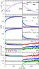 |
Fig. 5 Model B. a) The total luminosity of the envelope for τV = 1 and 2 and the unobscured star (thick black line). b) and c) Light curves Φλ(t) as defined by Eq. (15) in various Johnson filters. The black line is the normalized stellar light curve. d) Selected cloud colors for τV = 2. |
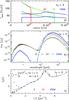 |
Fig. 6 Model B, τV = 2. a) Dust temperatures in the cloud 20, 70 and 150 days after the first photons enter the envelope. Upper lines: amorphous carbon, lower lines: silicate grains. b) The SED 5, 10, 20, 100 and 150 days after the cloud becomes visible. c) The extinction curve 1, 20, 80 and 150 days after the cloud becomes visible. Dots mark the effective, dashes the standard extinction curve. |
All graphs in Fig. 6 refer to τV = 2. The dust temperature distribution (Fig. 6a) is during the first 100 days after the entry of photons into the shell as in Model A. Later, when the influx of photons has stopped, the shell cools from the inside out. At t = 150 days, one has an inner zone of fairly constant temperature (for each dust component) so the photon density must be constant. Here heating proceeds only via scattered photons.
The SEDs in Fig. 6b increase in the first 100 days only a little at short wavelengths (as in Model A), but strongly in the far infrared. After 100 days, they decrease, most rapidly in the near IR (no dust emission, no multiple scattering) and not so rapidly, but still strongly in the optical where there is some multiple scattering. In the mid and far IR, the decline is softer. It is slowest at the longest wavelengths because this radiation comes from locations farthest from the star, at the edge of the shell.
As in Model A, immediately after the cloud becomes visible, the observed extinction curve, Eλ(t), almost coincides with the standard extinction curve ℰλ(t) (Fig. 6c). At short wavelengths (λ-1> 3 μm-1), there is afterwards little evolution. The photon statistics in this range are not as sound as one wishes because of the strong extinction, but deviations from the standard curve are expected to be small since the scattering properties in the UV and far UV are quite uniform (Fig. 1).
The evolution of Eλ(t) is very interesting for λ-1< 1.82 μm-1 (or λ> 0.55 μm). It approaches the effective extinction curve in the first 80 days. After 100 days, when the influx of direct stellar photons has ceased, only photons that have interacted with dust remain in the shell and of those there are much less in the near infrared than at B or V. Therefore, the gradient of Eλ switches sign in the NIR, Eλ(t) becomes positive and large as if there were strong extinction.
We learn from this model that even with standard dust, for which ℛV = 3.1, one can produce very small and even negative provided the star is dust-embedded and variable.
5.2. Supernova Ia
5.2.1. Model description
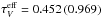
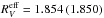
The star is now much more luminous () and the cloud is ten times bigger than in Model A and B. The inner cloud radius R1 is set equal to the dust evaporation radius Rev in Eq. (11) and R2 = 1 pc. The light travel time through the cloud is then 3.1 years. The stellar light curve is adapted to SN Ia and from Eq. (10). Again, the dust density in the cloud is constant and we consider, as before, the cases τV = 1 and 2 which imply  = 0.449 (0.957) and
  (1.847). A justification for the particular choice of parameters is given in Sect. 6, models with smaller and larger outer cloud radius, but otherwise identical, are presented in Sect. 5.2.6.
5.2.2. Light curves and colors
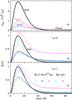 |
Fig. 7 SN Model 1 with R1 = 1.5 × 1017 cm, R2 = 1 pc and τV = 1 or 2. a) Bolometric luminosity of the envelope and the unobscured star. b) and c) Light curves Φλ(t) defined in Eq. (15) in selected bands and the normalized stellar light curve. |
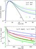 |
Fig. 8 SN Model 1. a) Light curves of the unobscured star and of the U and B band of the cloud, all normalized at their maximum. b) The long-term decline of the bolometric luminosity of the cloud (Lcl), the star (L∗) and the cloud fluxes in the B and I band. |
-
Whereas the bolometric luminosity of a stationary star isindependent of the amount of dust obscuration, the bolometricluminosity of the SN is reduced in its peak, relative to anunreddend SN, by a factor ~3 in the case τV = 1 and by a factor over 6 for τV = 2 (Fig. 7a). This reduction is caused by the larger travel times of photons that have been scattered or absorbed and reemitted. The bolometric fluxes integrated over time from t = 0 to ∞, or the areas under the three curves in Fig. 7a, are, of course, equal.
-
The optical light curves (UBVIJ) are also diminished in their maximum relative to a stationary obscured star of the same bolometric luminosity
(Figs. 7b and c). At U, the reduction amounts to 62% if τV = 2. Because of stochastic scattering, the escape of light from the SN shell is spread out over a period longer than the time of strong intrinsic SN emission (~50 days). The reduction in the first ~30 days is compensated by an enhancement later so that the total areas (from 0 to ∞) under the stellar and the UBVI curves in Figs. 7b and c are also equal, but it takes more than ten years until 99% of the photons have diffused out of the cloud. -
At J, there is already some weak dust emission (the computer code knows whether the detected photons come from the star or from grains), but it is unimportant. At K it is important so that the curve for K in Figs. 7b and c lies above the stellar curve (details depend sensitively on the dust evaporation temperature). At still longer wavelengths where dust emission is prevalent, a comparison of Φλ(t) with the stellar curve becomes meaningless.
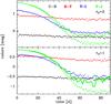
Fig. 9 SN Model 1. Selected colors of the cloud. The (green) V − J curves split after ~30 days. The upper branches, which have the larger scatter, give the true model results, in the lower ones, the dust radiation at J has been subtracted. They would apply if the luminosity or the dust evaporation temperature were lower. But the latter would also imply a smaller inner shell radius R1 (see Fig. 2) if we stick to R1 = Rev.
-
The occurence of the maximum in the UBV bands is delayed by 2 or 3 days. Because the curves are flat near maximum and have a minute numerical jitter, it is hard to read off a precise value.
-
The light curves of the optical bands are broadened with respect to the intrinsic stellar curve. The effect increases with τV and is best seen in Fig. 8a where the curves are normalized. The drop in U-brightness within 15 days after maximum, Δ15, is softened. It is reduced by about 0.5 mag (for τV = 1) relative to an unobscured star or an obscured one if the velocity of light were infinite.
-
To obtain at wavelength λ the total flux reduction at the light curve maximum relative to an unreddened supernova, one has to multiply the maximum value of the light curve Φλ(t) in Figs. 7b or c by
 . For instance, for τV = 1 (2), the light curve has near its maximum in the V band the value 0.63 (0.41),
  , (0.957), therefore fV = 0.638 (0.384) and the total reduction amounts to 0.638·fV = 0.407 (0.384·fV = 0.157).
 -
The behavior at wavelengths shorter than U (not shown) is similar, although τ is greater. At longer wavelengths, but before dust emission sets in, scattering becomes unimportant and Φλ(t) moves toward the solid stellar line.
-
The long-term fall-off over a period of two years of the bolometric cloud luminosity Lcl, and of the brightness in bands is much retarded compared to the intrinsic stellar light curve L∗(t) (Fig. 8b). All curves are normalized at their maximum. Especially the decline in Lcl is gentle. For τV = 2, Lcl ~ 5 × 10⁷L⊙, or 10% of the peak value, even after one year. The drop in the B band is more rapid and still more so at I where scattering is infrequent.
-
The change in cloud colors (Fig. 9) can be understood from what has been said regarding the colors in Fig. 5d: the discontinuity there at 100 days is here replaced by a gradual transition after the luminosity maximum. As the UBV light curves curves (and those at shorter wavelengths) are similar, there is not much spread in the colors (U − B) and (B − V), whereas in V − I and V − J it spans more than one magnitude.
-
The color excess EB − V(t) is obtained by subtracting from (B − V) the color (mB − mV)0 = 0.194 mag of the 10 000 K blackbody reference star.
5.2.3. Dust temperatures
The dust temperature profiles in Fig. 10 are taken at 300 and 600 days after stellar photons have entered the cloud and when it is not yet visible, and at 1145 days when it is visible near the brightness maximum.
All curves have a similar shape. At small radii, they are flat or have a gentle positive slope out to some point, rbump. The region with r<rbump is almost devoid of photons that have come straight from the star. The dust there is heated only by scattered photons and gradually cools as they diffuse out. At r>rbump, the temperature steeply rises, reaches a peak and then abruptly falls. The width of this bump is about 60 light days corresponding to the duration of the SN brightness peak (curve star in Fig. 7). In the bump, the dust is illuminated by stellar radiation emitted near the SN maximum which explains the temperature rise. After about 1180 days (not shown), the profiles are very similar to the blue curves, but the bump at the edge has gone.
The uniformity in the temperature after 1145 and more days is remarkable and very different from the profile of a steady source where Tdust roughly declines with r− 1 / 3. It does not, however, imply that the detected emission would be that of constant temperature dust because when the photons from the inner region have reached the surface S2 (Fig. 2), those from the outer region have already cooled.
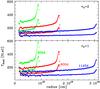 |
Fig. 10 SN Model 1. Dust temperatures at 300, 600 and 1145 days after the first photon has crossed the inner radius R1. For the same color, the upper curve refers to amorphous carbon grains, the lower one to silicates. |
5.2.4. Spectral energy distributions
Figure 11 shows SEDs at 5, 10, 40 and 80 days after visibility of the cloud, again for a distance of 10 Mpc. Notice the shift from an initially optical source near maximum to a predominantly mid infrared object after 40 and more days. The MIR fluxes fall off in step with the bolometric cloud luminosity and not as quickly as the optical fluxes whose time evolution can be best read off from Fig. 7. One can discern three broad resonances in the SEDs: an absorption dip at 0.22 μm and the silicate features at 10 and 18 μm.
FIR radiation detected from a SN cannot come from regions far away from it. Although the exploding star can heat dust even at a distance of 1 kpc to some 30 K and thus excite it to FIR emission, this emission will be too weak to be detected and too far offset in time to be related to the event.
The infrared radiaton can also not come from dust created in the explosion itself, although SN may well form grains. Dust formation can only happen after the expanding shell of supernova debris has cooled to the condensation temperature of dust. Assuming Tcond ~ 1200 K implies a minimum radius  cm or, for an expansion velocity off 2 × 10⁴ km s-1, a minimum time of ~500 days after the brightness maximum.
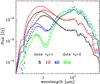 |
Fig. 11 SN Model 1. SEDs at 5, 10, 40 and 80 days after the cloud becomes visible for τV = 2 (crosses, triangles, squares) and τV = 1 (lines). |
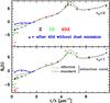 |
Fig. 12 SN Model 1. The extinction curve 2 (black points), 15 (green points) and 40 days (red points) after the cloud becomes visible. Without dust emission, the red points would fall in the infrared exactly on the blue curve. See also text. |
5.2.5. Extinction curves
Figure 12 shows the extinction curve Eλ(t) at 2, 15 (shortly after brightness maximum) and 40 days after the cloud becomes visible. These dates are partly chosen to sufficiently separate the curves one from another. Figure 12 also shows the standard (dashed) and effective (stippled) curve, and ℰλ, and the curve at t = 40 days that would be obtained if dust emission were absent (blue line). The blue line is not continued to short wavelengths but it perfectly fits there the “observed” red points.
As explained in Sect. 5.1.1, Eλ(t) is close to the standard curve ℰλ during the first few days. Later, there are moderate variations in the far UV, practically none between 1.8 and 4 μm-1, and some interesting ones in the near infrared. For λ-1< 1.82 μm-1 (or λ> 0.55 μm), Eλ(t) first rises, then turns into a steep fall. The rise is explained in Sect. 5.1.1. The slump is due to dust emission, which is absent in the low luminosity Model B of Sect. 5.1.2. It does therefore not represent the true extinction curve which is defined only for wavelengths without dust emission (but the observer has no means to verify that the light is free of dust radiation).
If the stellar luminosity or the dust evaporation temperature were sufficiently low, the curves in Fig. 12 would qualitatively look in the NIR as those in Fig. 6c and after 40 days, the red points in Fig. 12 would in the infrared fall exactly on the blue curve.
Note that the near infrared variability of the extinction curve is an indicator of circumstellar dust.
5.2.6. Other SN Ia models
There is an endless manifold of how the envelope (Fig. 2) may be structured, but the fact that our models are spherically symmetric is probably not a very severe limitation (the neglect of clumpiness may be more important) because during the first days only photons will be detected that left the star in a cone directed towards the observer. Photons fired to the sides or the rear will only be registered later.
We show in Figs. 13 to 20 results for two other spherically symmmetric and homogeneous shell configurations with the same extinction optical depth τV = 1 or 2, but with different outer radii (R2 = 0.5 pc in SN Model 2, R2 = 2 pc in SN Model 3); in all three cases R1 = 1.5 × 1017 cm. After the discussion of SN Model 1, the pictures are self-explicative. Obviously, when the cloud gets bigger dust temperatures decrase and the SED changes correspondingly. When R2 ≫ 1 pc, the effects of time delay disappear altogether, and when the cloud is smaller than 1 pc, so that the light travel time through the shell becomes comparable to the time over which the SN luminosity changes appreciably, they grow.
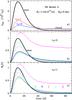 |
Fig. 13 SN Model 2. Like Model 1, but with smaller outer cloud radius R2 = 0.5 pc. The values of |
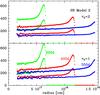 |
Fig. 14 SN Model 2. Dust temperatures at indicated days after first photons cross inner radius R1. See caption Fig. 10. |
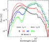 |
Fig. 15 SN Model 2. SEDs at indicated days after cloud becomes visible for τV = 2 (crosses, triangles, squares) and τV = 1 (lines). See caption Fig. 11. |
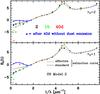 |
Fig. 16 SN Model 2. The extinction curve at indicated days after the cloud becomes visible. In the blue curve, dust emission has been subtracted. See caption Fig. 12. |
 |
Fig. 17 SN Model 3. Like Model 1, but with larger outer cloud radius R2 = 2 pc. The values of |
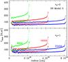 |
Fig. 18 SN Model 3. Dust temperatures at indicated days after the first photons have crossed the inner radius R1. See caption Fig. 10. |
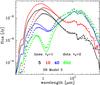 |
Fig. 19 SN Model 3. SEDs at indicated days after the cloud becomes visible for τV = 2 (crosses, triangles, squares) and τV = 1 (lines). See caption Fig. 11. |
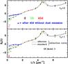 |
Fig. 20 SN Model 3. The extinction curve at indicated days after the cloud becomes visible. In the blue curve, dust emission has been subtracted. See caption of Fig. 12. |
5.2.7. The luminosity deduced by an observer
Flux measurements integrated over all wavelengths yield for a dust-enveloped supernova near its maximum a total luminosity much smaller (six times for τV = 2) than what would be derived for a stationary source of the same luminosity within the same dust envelope (Fig. 7a). Without further reflections why there is far infrared emission at all, one would grossly underestimate the intrinsic SN power.
At optical wavelengths, the brightness is also weaker than of a steady source of the same luminosity within the same dust envelope, not so much, but still up to a factor of three (Figs. 7b and c). One might therefore surmise that, applying optical photometric methods, an observer will also underrate the intrinsic UBV brightness of the SN. However, here the situation is more sophisticated.
First, the observer has to deredden the star (which is not necessary for the bolometric luminosity and, strictly speaking, not possible when the extinction curve is variable). But let us suppose he proceeds in the usual way. He measures at V the flux  (see Eq. (16)), the color B − V, and subtracts from it the color (B − V)0 = 0.194 of the reference star to obtain the color excess EB − V. Then he converts EB − V into AV using RV. Without any assumptions, he has to derive RV from the infrared part of the extinction curve; the result, even for standard dust, will depend on when the observations are done (see Fig. 12), Or one puts, as usual, RV = 3.1. In any case, the infered intrinsic stellar flux,
  , is
, is  (17)(because τV = AV/ 1.086). Results for RV = 3.1 are plotted in Fig. 21 for SN Models 1 to 3 and a fourth one. We recall that if the velocity of light were infinite,
  would exactly match the undiminished stellar brightness (curve marked star in Fig. 7b). We see that the observer tends to overestimate the intrinsic stellar brightness near and shortly after the maximum, but not by much. Only later the estimate becomes unacceptable.
SN Model 4 (red triangles in Fig. 21) is identical to SN Model 1 except for the dust properties. But they differ only in the asymmetry factor gλ and the albedo ωλ, two quantities not well determined. The extinction coefficient,  , is unchanged, so the extinction curve ℰλ would not be affected. In particular, we have lowered ωV from 0.586 to 0.42, gV from 0.544 to 0.3 and increased ωB from 0.524 to 0.65 and gB from 0.534 to 0.7.
We explain what happens in the V-band. Lowering ωV (while keeping KV constant) increases the fraction of absorbed and decreases that of scattered radiation. At first, the drop in ωV has no effect, but after a few days it reduces the flux compared to the one with the standard ωV because  is greater and scattered photons have not yet arrived. Later the gap between the normal and the modified ω widens because the chance of a scattered photon to be absorbed increases in time. Eventually, the flux at V gets smaller and the infered intrinsic maximum SN brightness is progressively underestimated. Similar arguments apply when scattering becomes more isotropic (smaller gV).
In the end, this reduces EB − V and therefore the intrinsic (unreddened) brightness at V derived by an observer. EB − V can even vanish or become negative. The light is then attenuated, but not reddened and the intrinsic V-brightness of the star would be underrated.
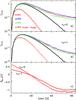 |
Fig. 21 a) and b): the V-brightness of the star from Eq. (17) as deduced by an observer in units of the true maximum stellar brightness. The true stellar brightness is given by the solid line. The models differ in size and, for SN4 also in the scattering properties of the dust. SN4 is otherwise identical to SN1. c) The color excess EB − V(t) for SN4. |
6. Discussion
The analysis of stellar photometry in this paper can be applied to any dust enshrouded variable source. The major motivation came, however, from the discussion around dark energy. The dimming of type Ia supernovae, used as standard candles, plays, among other vital evidence, still the dominant role in the defense of this mysterious force. Although its existence is firmly established in the literature (see reviews by Riess 2000; Leibundgut 2001; Frieman et al. 2008; Goobar & Leibundgut 2011), all arguments casting doubt on the hypothesis should be thoroughly falsified because of its truly paramount importance.
In order to explain our choice of sizes and optical depths of the model cloud, we note that the effects discussed here for the extinction curve and the optical light curves require an optical depth of the envelope around τV = 1. It must not be small, nor large as the effects would then not be detectable. If the envelope radius, R, is much bigger than 1 pc, while keeping τV fixed, it behaves like any foreground cloud, if it is much smaller, the source is dominated even at 1 μm by dust emission.
If the cloud is a homogeneous sphere, the gas mass contained in it equals Mg = 4πR2τV/ 3KV, where KV is the extinction coefficient per g of IM. Using KV ≃ 200 cm2, the approximate value in the Milky Way, R = 1 pc and τV = 1 lead to Mg ~ 100M⊙ and a density of ~1000 gas atoms per cm3. Such numbers for the cloud mass and density are not associated with the immediate environment of SN Ia, which are not young objects. The evidence is rather that when SN Ia suffer from dust extinction, it happens somewhere in the interstellar medium of the host galaxy and not in the circumstellar material around the progenitor system (Phillips et al. 2013). A possible, although unlikely configuration would be dense stellar clusters, similar to globular clusters, with ~103 or more stars per pc3 and an IM mass fraction of a few per cent. A supernova releasing a kinetic energy of 1050 erg would disperse the gas, but the dispersal becomes effective only after ~100 years when the shock front has traversed the envelope. Mass loss from the other stars in the cluster might replenish the expelled gas before the next supernova explodes.
The models outline only the general photometric features. They can be refined and the parameter space extended in many directions: dust properties; shell structure, non-uniform density, possibly clumps and, foremost, a realistic SN spectral luminosity, L∗ ,λ(t), instead of the 104 K blackbody. Whether the basic findings, listed below, will stay in force or even become more pronounced is unclear, but the simplistic model of this paper may then still serve, by way of comparison, to identify the underlying mechanisms.
We do not to propose that SN Ia at an early epoch are enshrouded by clouds nor that the scattering properties of the dust there is anomalous compared to the Milky Way, we rather think it unlikely. But when juxtapositioned to something outside the present physical realm, even a wild speculation is permitted and the theoretical analysis of SN photometry may deserve some more attention.
7. Summary
-
1.
A stationary star in a spatially unresolved dusty envelope ofextinction optical depth τ suffers an attenuation exp( − τeff) that is less than exp( − τ). The observed (effective) extinction curve
(Eq. (3)) differs from ℰλ of Eq. (1) and the ratio of total over selective extinction, , is smaller than ℛV. This is an effect only of radiative transfer and not of dust properties. -
2.
A Monte Carlo method, based on the scheme of Bjorkman & Wood (2001) and using standard Milky Way dust, is presented to treat variable sources.
-
3.
If the source is variable one can produce with standard dust almost any shape of the extinction curve in the infrared, and thus almost any value of
, while the UV part of the extinction curve does not change much. In pencil beam observations, on the other hand, τeff = τ and one always observes the standard extinction curve with ℛV = 3.1, even if the star is variable. -
4.
The bolometric flux from a shell, filled with standard dust, of optical thickness τV ~ 1 and radius ~1 pc, centered around a variable star with a luminosity and light curve like a supernova, is much reduced in its peak relative to the star, and after t> 30 days it is much enhanced (Fig. 7a).
-
5.
Likewise, the flux at an optical wavelength near the SN peak is considerably smaller than the flux from a stationary star of the same luminosity and in the same environment. After t> 30 days, the flux is enhanced relative to the stationary star (Figs. 7b and c). The optical light curves are broadened and their maxima slightly shifted (Fig. 8a), as already noted by Amanullah & Goobar (2011).
-
6.
The temperature profile of the shell, when it becomes visible, is very uniform, but for a leading edge (Fig. 10). After ~20 days, the edge has disappeared, the temperature stays uniform and gradually declines. Heating comes then from scattered photons.
-
7.
The SED is initially dominated by the optical and later by the FIR region. The FIR flux abates very slowly.
-
8.
The extinction curve is time-variable (Fig. 12). Initially it coincides with ℰλ of Eq. (1). Later relevant modifications appear for λ> 0.55 μm. The “observed” points in the NIR are for λ ≥ 1.2 μm contaminated by dust emission. This contamination can be reduced or eliminated when the dust evaporation temperature or the SN luminosity is lowered.
-
9.
Dereddening the star via the color excess EB − V to obtain the intrinsic SN luminosity, one finds near maximum approximately the correct value; later on, the intrinsic luminosity is overestimated. Details depend on the not well known scattering properties at B and V. Changing them, without changing the extinction coefficient, can lead to a severe underestimate of the intrinsic maximum luminosity (Fig. 21).
-
10.
Iron grains have, because of their high reflectivity, also the property to attenuate light without much reddening it (Fig. A.1).
-
11.
As a side point, ℛV can be brought below 2 if the carbon dust consists solely of graphites.
Acknowledgments
I am much obliged to the anomymous referee, Rolf Chini, Bruno Leibundgut, Peter Schneider, Ralf Siebenmorgen, and Malcolm Walmsley for their valuable assistance.
References
- Aguirre, A. 1999a, ApJ, 512, L19 [NASA ADS] [CrossRef] [Google Scholar]
- Aguirre, A. 1999b, ApJ, 525, 583 [NASA ADS] [CrossRef] [Google Scholar]
- Amanullah, R., & Goobar, A. 2011, ApJ, 735, 20 [NASA ADS] [CrossRef] [Google Scholar]
- Amanullah, R., Goobar, A., Johansson, D. P., et al. 2014, ApJ, 788, L21 [NASA ADS] [CrossRef] [Google Scholar]
- Bjorkman, J. E., & Wood, K. 2001, ApJ, 554, 615 [NASA ADS] [CrossRef] [Google Scholar]
- Chevalier, R. A. 1986, ApJ, 308, 225 [NASA ADS] [CrossRef] [Google Scholar]
- Fischera, J., & Schmidt, R. 2009, ASP Conf., 414, 266 [NASA ADS] [Google Scholar]
- Frieman, J. A., Turner, M. S., & Huterer, D. 2008, ARA&A, 46, 385 [NASA ADS] [CrossRef] [Google Scholar]
- Foley, R. J., Fox, O. D., McCully, C., et al. 2014, MNRAS, in press [Google Scholar]
- Goobar, A. 2008, ApJ, 686, L103 [NASA ADS] [CrossRef] [Google Scholar]
- Goobar, A., & Leibundgut, B. 2011, Ann. Rev. Nucl. Part. Sci., 61, 251 [NASA ADS] [CrossRef] [Google Scholar]
- Hsiao, E. Y., Conley, A., Howell, D. A., et al. 2007, ApJ, 663, 1187 [NASA ADS] [CrossRef] [Google Scholar]
- Johnson, P. B., & Christy, R. W. 1974, Phys. Rev. B, 9, 5056 [NASA ADS] [CrossRef] [Google Scholar]
- Krügel, E. 2006, An Introduction to the Physics of Interstellar Dust (Taylor & Francis) [Google Scholar]
- Krügel, E. 2009, A&A, 493, 385 [NASA ADS] [CrossRef] [EDP Sciences] [Google Scholar]
- Laor, A., & Draine, B. T. 1993, ApJ, 402, 441 [NASA ADS] [CrossRef] [Google Scholar]
- Leibundgut, B. 2001, ARA&A, 39, 67 [NASA ADS] [CrossRef] [Google Scholar]
- Leibundgut, B. 2011, ARA&A, 46, 386 [Google Scholar]
- Leksina, I. E., & Penkina, N. V. 1967, Fiz. Met. Metalloved, 23, 344 [Google Scholar]
- Mathis, J. S., Rumpl, W., & Nordsieck, K. H. 1977, ApJ, 217, 425 [NASA ADS] [CrossRef] [Google Scholar]
- Nobili, S., & Goobar, A. 2008, A&A, 487, 19 [NASA ADS] [CrossRef] [EDP Sciences] [Google Scholar]
- Ordal, M. A., Bell, R. J., Alexander, R. W., Newquist, L. A., & Querry, M. A. 1988, Appl. Opt., 27, 1203 [NASA ADS] [CrossRef] [PubMed] [Google Scholar]
- Parodi, B. R., Saha, A., Sandage, A., & Tammann, G. A. 2000, ApJ, 540, 634 [NASA ADS] [CrossRef] [Google Scholar]
- Patat, F., Taubenberger, S., Cox, N. L. J., et al. 2014, A&A, submitted [Google Scholar]
- Phillips, M. M., Lira, P., Suntzeff, N. B., et al. 1999, AJ, 118, 1766 [NASA ADS] [CrossRef] [Google Scholar]
- Phillips, M. M., Simon, J. D., Morrell, N., et al. 2013, ApJ, 779, 1 [NASA ADS] [CrossRef] [Google Scholar]
- Riess, A. G. 2000, PASP, 112, 1284 [NASA ADS] [CrossRef] [Google Scholar]
- Riess, A. G., Strolger, L. G., Casertano, S., et al. 2007, ApJ, 659, 98 [NASA ADS] [CrossRef] [Google Scholar]
- Wang, L. 2005, ApJ, 635, L33 [NASA ADS] [CrossRef] [Google Scholar]
- Weingartner, J. C., & Draine, B. T. 2001, ApJ, 548, 295 [NASA ADS] [Google Scholar]
- Zubko, V. G., Mennella, V., Colangeli, L., et al. 1996, MNRAS, 282, 1321 [NASA ADS] [CrossRef] [Google Scholar]
Appendix A: Small ℛV
Although the dependence of ℛV on dust properties is not the topic of this paper (where it is constant and equal to 3.1), we briefly remark on its general behavior because values are reported towards extragalactic supernovae that are smaller than anywhere in the Milky Way (Phillips et al. 2013; Nobili & Goobar 2008). Of course, they may refer to , and not to ℛV proper.
If the grains are much bigger than the wavelength, the extinction efficiency at any such wavelength is close to 2, no matter what they are made of (Babinet’s theorem). KB − KV is then small and ℛV large, it may be positive or negative. If the grains are only fairly big (radius a = 1...3 × 10-5 cm), Mie theory yields numbers that fluctuate strongly. Very small grains of silicate have ℛV ~ 4.3, of amorphous carbon ℛV ~ 1.9, of graphite ℛV ~ 2.1.
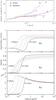 |
Fig. A.1 Top: optical constants n and k of metallic iron (L from Leksina & Penkina 1967; J from Johnson & Christy 1974; O from Ordal et al. 1988). Bottom: extinction efficiency Qext of iron spheres, their albedo ω and the asymmetry factor g, as a function of grain radius for λ = 0.36,0.44,0.55,0.7,1.25 and 2.2 μm, using a good-will average of the (n,k)-data in the upper box. |
Obviously, one needs for ℛV a mixture of grain sizes (and composition). This is not totally trivial because a spread in particle sizes (the MRN distribution, Mathis et al. 1977) was needed to explain the extinction curve over a large wavelength interval (from 0.1 to 10 μm), and not just for two wavelengths (B and V) lying close together. The surprising constancy of ℛV in the Milky Way (despite the many exceptions) is usually interpreted to be due to similar creation and destruction processes plus effective mixing.
One means to make ℛV small or even press it below 2 is to turn all or most of the amorphous carbon into graphite, without changing the mass fractions faC + fgr orfSi, nor the sizes of the silicates. Such a metamorphosis from an amorphous into a semi-crysralline state (graphite) can happen when irregularly built carbon particles are exposed to hard radiation; it is the way graphites are believed to be made in the Milky Way. In the process, bigger graphite grains are created. If, for example, agr = 0.015...0.064 μm, one gets ℛV = 1.76, at least, on the computer. If such an idea has a touch of reality, small ℛV towards supernovae extinguished in the host galaxy should be limited to active galaxies with plenty of hard photons.
Appendix B: Further examples of attenuation without reddening
Two further examples where the full amount of attenuation will not be appreciated in optical photometry because it is not accompanied by a corresponding degree of reddening are a) big grains because of Babinet’s theorem. However, with regard distant SN Ia, their presence can be excluded, at least, in the intergalactic medium (Aguirre 1999a,b; Goobar et al. 2002; Riess et al. 2007). And b) Iron particles. If they are not too small (radius a ≳ 0.1 μm), they have at B and V almost the same extinction coefficient Kλ (Fig. A.1) and they will redden even a substantially attenuated star only weakly. Because iron grains are very reflective and have similar albedo ωλ, the variations of the color B − V in time will be small if they are located in a circumstellar envelope. The production of iron grains (most likely in SN Ia) and their abundance relative to other solid particles is an entirely different topic.
All Figures
|
Fig. 1 a) Abedo ω (blue squares) and asymmetry factor, g, (green triangles) for standard dust defined in Sect. 3.1; it is used in all models of this paper. Points mark frequently used wavelengths, like UBVRI ...b) Standard dust produces in pencil beam observations the standard extinction curve ℰλ (red triangles). The black squares display the effective extinction curve assuming a Henyey-Greenstein phase function towards an unresolved shell source (see Fig. 2) with τV = 2 and other parameters as described in Sect. 5.2.1. |
| In the text | |
|
Fig. 2 Sketch of a spherical dust envelope around a SN and three possible photon flight paths. Their direction changes after an absorption or scattering event. The inner and outer radii and surfaces of the envelope are R1,R2, and S1,S2, respectively. R1 is equal to the evaporation radius Rev. |
| In the text | |
|
Fig. 3 Model A. a) The total luminosity of the unobscured star (thick black line) and the envelope for τV = 1 and 2. b) and c) Light curves Φλ(t) as defined by Eq. (15) in various Johnson filters. Here and in the following figures, the bands can be identified by their colors. The black horizontal line is the normalized light curve of the star. For further parameters, see text. |
| In the text | |
|
Fig. 4 Model A, τV = 1. a) Dust temperatures in the cloud 20, 70 and 150 day after the first photons enter the envelope. Upper lines: amorphous carbon, lower lines: silicate grains. b) The SED 5, 10, 20, 40 and 150 days after the cloud becomes visible. c) The extinction curve 1, 20 and 150 days after the cloud becomes visible. The dotted line marks the effective, the dashed one the standard extinction curve. |
| In the text | |
|
Fig. 5 Model B. a) The total luminosity of the envelope for τV = 1 and 2 and the unobscured star (thick black line). b) and c) Light curves Φλ(t) as defined by Eq. (15) in various Johnson filters. The black line is the normalized stellar light curve. d) Selected cloud colors for τV = 2. |
| In the text | |
|
Fig. 6 Model B, τV = 2. a) Dust temperatures in the cloud 20, 70 and 150 days after the first photons enter the envelope. Upper lines: amorphous carbon, lower lines: silicate grains. b) The SED 5, 10, 20, 100 and 150 days after the cloud becomes visible. c) The extinction curve 1, 20, 80 and 150 days after the cloud becomes visible. Dots mark the effective, dashes the standard extinction curve. |
| In the text | |
|
Fig. 7 SN Model 1 with R1 = 1.5 × 1017 cm, R2 = 1 pc and τV = 1 or 2. a) Bolometric luminosity of the envelope and the unobscured star. b) and c) Light curves Φλ(t) defined in Eq. (15) in selected bands and the normalized stellar light curve. |
| In the text | |
|
Fig. 8 SN Model 1. a) Light curves of the unobscured star and of the U and B band of the cloud, all normalized at their maximum. b) The long-term decline of the bolometric luminosity of the cloud (Lcl), the star (L∗) and the cloud fluxes in the B and I band. |
| In the text | |
|
Fig. 9 SN Model 1. Selected colors of the cloud. The (green) V − J curves split after ~30 days. The upper branches, which have the larger scatter, give the true model results, in the lower ones, the dust radiation at J has been subtracted. They would apply if the luminosity or the dust evaporation temperature were lower. But the latter would also imply a smaller inner shell radius R1 (see Fig. 2) if we stick to R1 = Rev. |
| In the text | |
|
Fig. 10 SN Model 1. Dust temperatures at 300, 600 and 1145 days after the first photon has crossed the inner radius R1. For the same color, the upper curve refers to amorphous carbon grains, the lower one to silicates. |
| In the text | |
|
Fig. 11 SN Model 1. SEDs at 5, 10, 40 and 80 days after the cloud becomes visible for τV = 2 (crosses, triangles, squares) and τV = 1 (lines). |
| In the text | |
|
Fig. 12 SN Model 1. The extinction curve 2 (black points), 15 (green points) and 40 days (red points) after the cloud becomes visible. Without dust emission, the red points would fall in the infrared exactly on the blue curve. See also text. |
| In the text | |
|
Fig. 13 SN Model 2. Like Model 1, but with smaller outer cloud radius R2 = 0.5 pc. The values of |
| In the text | |
|
Fig. 14 SN Model 2. Dust temperatures at indicated days after first photons cross inner radius R1. See caption Fig. 10. |
| In the text | |
|
Fig. 15 SN Model 2. SEDs at indicated days after cloud becomes visible for τV = 2 (crosses, triangles, squares) and τV = 1 (lines). See caption Fig. 11. |
| In the text | |
|
Fig. 16 SN Model 2. The extinction curve at indicated days after the cloud becomes visible. In the blue curve, dust emission has been subtracted. See caption Fig. 12. |
| In the text | |
|
Fig. 17 SN Model 3. Like Model 1, but with larger outer cloud radius R2 = 2 pc. The values of |
| In the text | |
|
Fig. 18 SN Model 3. Dust temperatures at indicated days after the first photons have crossed the inner radius R1. See caption Fig. 10. |
| In the text | |
|
Fig. 19 SN Model 3. SEDs at indicated days after the cloud becomes visible for τV = 2 (crosses, triangles, squares) and τV = 1 (lines). See caption Fig. 11. |
| In the text | |
|
Fig. 20 SN Model 3. The extinction curve at indicated days after the cloud becomes visible. In the blue curve, dust emission has been subtracted. See caption of Fig. 12. |
| In the text | |
|
Fig. 21 a) and b): the V-brightness of the star from Eq. (17) as deduced by an observer in units of the true maximum stellar brightness. The true stellar brightness is given by the solid line. The models differ in size and, for SN4 also in the scattering properties of the dust. SN4 is otherwise identical to SN1. c) The color excess EB − V(t) for SN4. |
| In the text | |
|
Fig. A.1 Top: optical constants n and k of metallic iron (L from Leksina & Penkina 1967; J from Johnson & Christy 1974; O from Ordal et al. 1988). Bottom: extinction efficiency Qext of iron spheres, their albedo ω and the asymmetry factor g, as a function of grain radius for λ = 0.36,0.44,0.55,0.7,1.25 and 2.2 μm, using a good-will average of the (n,k)-data in the upper box. |
| In the text | |
Current usage metrics show cumulative count of Article Views (full-text article views including HTML views, PDF and ePub downloads, according to the available data) and Abstracts Views on Vision4Press platform.
Data correspond to usage on the plateform after 2015. The current usage metrics is available 48-96 hours after online publication and is updated daily on week days.
Initial download of the metrics may take a while.