© ESO, 2015

1. Introduction

By now it is well understood that stars form out of the gravitational condensation of cold and dense molecular cores, which are very structured in density and in velocity (Larson 1981; Falgarone & Phillips 1990). In parallel, it has also been argued that most stars live in binaries or multiple systems (e.g., Duquennoy & Mayor 1991; Goodwin et al. 2007). It is therefore natural to assume that owing to these internal velocities and density enhancements, a core typically fragments at a certain stage of its collapse and eventually produces two or more stars.

From an observational perspective, the matter can be elucidated by registering the degree of multiplicity at different stages of the core contraction. Most data for early stellar multiplicity are available for Class I/II objects, in other words, for protostars with almost no trace of their initial envelope left (Ghez et al. 1993; Patience et al. 2002; Duchêne et al. 2004, 2007). But, to clarify the dependence on the initial physical properties and internal structure of a core, one must allude to even earlier phases in the collapse (Class 0 objects), when the protostars are still largely embedded in their parental core (Andre et al. 1993, 2000). Although challenging because of the obscuration from the envelope, there have been numerous attempts to constrain stellar multiplicity that early in the collapse stage of a core (Chen et al. 2008; Girart et al. 2009; Duchêne et al. 2004, 2007; Jørgensen et al. 2007). The results show an increase in the number of fragments from the Class 0 to the Class I stage, which is evidence that suggests that fragmentation is favored either in the Class 0 stage or very shortly afterward (Maury et al. 2010).

There have been also numerous theoretical studies, both of the collapse process and of the fragmentation during collapse. Ebert (1955) and Bonnor (1956) independently derived an analytic criterion for a static isothermal sphere to be stable against gravitational collapse. In their numerical simulations of collapsing, initially uniform isothermal spheres, Larson (1969) and Penston (1969) found a one-dimensional, self-similar solution (called LP solution or flow in the following). If x is the self-similar variable of the profile, this solution describes a cloud with a flat density profile that turns into a x^-2 dependence toward infinity and a velocity profile proportional to x. It was later discovered by Shu (1977) that this solution is a member of a whole family of self-similar collapse solutions, many of which contain critical points. In that paper, he arrived at the conclusion that an initially centrally condensed cloud will collapse from the inside out, establishing an expansion wave. This behavior was integrated into a more complete picture of the collapse and the behavior of self-similar collapse solutions by Whitworth & Summers (1985).

The stability of the collapse solutions is understood to a much lesser extent. For the case of a static, uniform, presureless spherical cloud, Hunter (1964) showed that there is an unstable shell mode that grows like (t₀ − t)^-1, where t is the time and t₀ the time at which collapse occurs.

Hanawa & Matsumoto (1999, HM99 in the following) performed a stability analysis of the LP flow using a shooting method. In this type of analysis, one starts integrating the equations from one boundary and varies some parameters until the solution at the other boundary matches the desired conditions there. They came to the conclusion that the solution is stable overall, with the exception of a slowly growing l = 2 mode (where l the azimuthal wave number of a spherical harmonic perturbation) with a growth rate of 0.354. This very weak instability is consistent with the analysis by Ori & Piran (1988), who derived a stability criterion for self-similar isothermal collapse flows that is based on the gradient of the radial velocity close to the critical point. According to that criterion, a homogeneous isothermal sphere is an unstable configuration that could naturally converge to a (generally much stabler) Larson-Penston type flow.

While quite interesting, this result poses a few questions. One is that the growth rate is rather slow, so it is unclear whether perturbations can really grow sufficiently (see Sect. 5). Another issue is that only the l = 2 mode was found to be unstable, since HM99 report the nonexistence of eigenvectors for higher values of l. Finally, no total eigenvector has been calculated for the spherical mode. Altogether, this suggests that the stability analysis of a collapsing cloud is not yet complete.

On the other hand, there is abundant literature on numerical simulations of the fragmentation of rotating and/or turbulent cores. Boss & Bodenheimer (1979) studied the fate of an l = 2 perturbation on a collapsing core, and Burkert & Bodenheimer (1993) repeated the experiment, finding that a filament connecting the fragments should develop. (This experiment has been repeated many times since and is used extensively as a code testing tool.) A criterion for fragmentation in the presence of rotation was provided by the semi-analytical work of Tohline (1981), quantifying thermal support with the virial parameter α and the rotational versus gravitational energy in the cloud with the corresponding parameter β. The quantity αβ has since been used repeatedly to delimit the conditions for fragmentation (Miyama et al. 1984; Hachisu & Eriguchi 1984; Tsuribe & Inutsuka 1999; Tohline 2002, for instance), and it was found that αβ< 0.1−0.2 typically leads to fragmentation.

At the same time, increasingly more complex direct simulations of the collapse and fragmentation processes have been performed, including the internal and external thermal pressure of the core, rotation (Myhill & Kaula 1992; Cha & Whitworth 2003; Matsumoto & Hanawa 2003; Hennebelle et al. 2004; Machida et al. 2008; Commerçon et al. 2008), magnetic fields (Banerjee & Pudritz 2006; Price & Bate 2007; Hennebelle & Teyssier 2008; Boss & Keiser 2013), and turbulence (Klessen et al. 1998; Klessen & Burkert 2001; Offner et al. 2008; Bate 2009; Joos et al. 2013), which seem to affect the number of fragments and their separation. Girichidis et al. (2011) conducted a parameter study in which they varied the initial density profile of the core and the level of turbulence. They provide evidence of the strong influence of the mean radial density profile to the result of the collapse.

Given the abundance and complexity of the existing models for fragmentation, it is somewhat surprising that there is so little to be said for the stability of a solution that is as simple as the homologous, uniform, isothermal collapse. It is clear that this solution has limited applicability to real cores, which are sometimes far from isothermal spheres and do host turbulent motions and magnetic fields, which are all potentially important and complex effects that can substantially alter the behavior of the solution. However, a study of its linear stability offers important insight into the principal mechanisms causing fragmentation, since it does not suffer from the complexity of nonlinear effects and can contribute to the overall understanding of core collapse.

In the present paper we rectify by performing a linear stability analysis of this flow. Our study shows that the homologous solution is indeed unstable and we obtain the corresponding growth rates. This analysis is presented in Sects. 2 and 3. In the fourth section we present numerical simulations of a uniform dense core subject to a spherical perturbation and we look for the range of parameters for which it is unstable. We measure the growth rate of the shell mode (a spherically symmetric perturbation), as well as higher-order spherical harmonic perturbations and find them to be in good agreement with the result of our linear analysis. The fifth section discusses the implications of our results and proposes further interpretation. The sixth section concludes the paper.

2. Stability analysis: the spherical case

2.1. Equations and self-similarity

We investigate the stability of a collapsing isothermal sphere against linear perturbations. Given the symmetry of the problem, we start with the equations of hydrodynamics in spherical coordinates in one dimension: 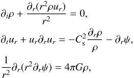$\begin{array}{ccc}& & {\mathit{\partial }}_{\mathit{t}}\mathit{\rho }\mathrm{+}\frac{{\mathit{\partial }}_{\mathit{r}}\mathrm{\left(}{\mathit{r}}^{\mathrm{2}}\mathit{\rho }{\mathit{u}}_{\mathit{r}}\mathrm{\right)}}{{\mathit{r}}^{\mathrm{2}}}\mathrm{=}\mathrm{0}\mathit{,}\\ & & {\mathit{\partial }}_{\mathit{t}}{\mathit{u}}_{\mathit{r}}\mathrm{+}{\mathit{u}}_{\mathit{r}}{\mathit{\partial }}_{\mathit{r}}{\mathit{u}}_{\mathit{r}}\mathrm{=}\mathrm{-}{\mathit{C}}_{\mathrm{s}}^{\mathrm{2}}\frac{{\mathit{\partial }}_{\mathit{r}}\mathit{\rho }}{\mathit{\rho }}\mathrm{-}{\mathit{\partial }}_{\mathit{r}}\mathit{\psi ,}\\ & & \frac{\mathrm{1}}{{\mathit{r}}^{\mathrm{2}}}{\mathit{\partial }}_{\mathit{r}}\mathrm{\left(}{\mathit{r}}^{\mathrm{2}}{\mathit{\partial }}_{\mathit{r}}\mathit{\psi }\mathrm{\right)}\mathrm{=}\mathrm{4}\mathit{\pi G\rho ,}\end{array}$(1)where ρ the gas mass density, u_r the radial velocity, and ψ the gravitational potential. It is well known (Larson 1969; Penston 1969; Shu 1977) that this system admits self-similar solutions of the form 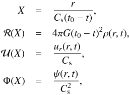$\begin{array}{ccc}\mathit{X}& \mathrm{=}& \frac{\mathit{r}}{{\mathit{C}}_{\mathrm{s}}\mathrm{(}{\mathit{t}}_{\mathrm{0}}\mathrm{-}\mathit{t}\mathrm{)}}\mathit{,}\\ \mathrm{ℛ}\mathrm{\left(}\mathit{X}\mathrm{\right)}& \mathrm{=}& \\ \mathrm{𝒰}\mathrm{\left(}\mathit{X}\mathrm{\right)}& \mathrm{=}& \frac{{\mathit{u}}_{\mathit{r}}\mathrm{\left(}\mathit{r,t}\mathrm{\right)}}{{\mathit{C}}_{\mathrm{s}}}\mathit{,}\\ \mathrm{\Phi }\mathrm{\left(}\mathit{X}\mathrm{\right)}& \mathrm{=}& \frac{\mathit{\psi }\mathrm{\left(}\mathit{r,t}\mathrm{\right)}}{{\mathit{C}}_{\mathrm{s}}^{\mathrm{2}}}\mathit{,}\end{array}$(2)where the density ℛ, the radial velocity , and the gravitational potential, Φ are functions of the self-similar variable X, C_s is the sound speed, and G the gravitational acceleration. Among the various solutions known in the literature the simplest is the homologous solution 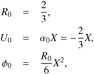$\begin{array}{ccc}{\mathit{R}}_{\mathrm{0}}& \mathrm{=}& \frac{\mathrm{2}}{\mathrm{3}}\mathit{,}\\ {\mathit{U}}_{\mathrm{0}}& \mathrm{=}& \\ {\mathit{\phi }}_{\mathrm{0}}& \mathrm{=}& \frac{{\mathit{R}}_{\mathrm{0}}}{\mathrm{6}}{\mathit{X}}^{\mathrm{2}}\mathit{,}\end{array}$(3)which describes a cloud with a uniform density R₀ and a velocity field proportional to X with a slope α₀. Clearly, like other self-similar profiles, this solution is only valid within certain spatial and temporal limits, as both the mass and the velocity diverge for large values of X. In addition, in a real collapse situation there is a rarefaction wave propagating outwards (Tsuribe & Inutsuka 1999; Truelove et al. 1997), which breaks the self-similarity. In order then for this solution to remain valid the gas has to be cold enough for the collapse to happen before the rarefaction wave can reach the center. Then Eqs. (3) can be used to describe the inner parts of the cloud.

The simplicity of this profile and the fact that it describes the center of a cold core quite accurately make it a popular initial condition for numerical simulations (Larson 1969; Price & Bate 2007; Commerçon et al. 2008; Boss & Keiser 2013, for example). It is therefore both interesting and relevant to perform a stability analysis of this solution and to confront the analytical results with numerical simulations.

We first look for perturbations of the form 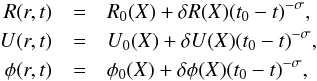$\begin{array}{ccc}\mathit{R}\mathrm{\left(}\mathit{r,t}\mathrm{\right)}& \mathrm{=}& {\mathit{R}}_{\mathrm{0}}\mathrm{\left(}\mathit{X}\mathrm{\right)}\mathrm{+}\mathit{\delta R}\mathrm{\left(}\mathit{X}\mathrm{\right)}\mathrm{(}{\mathit{t}}_{\mathrm{0}}\mathrm{-}\mathit{t}{\mathrm{)}}^{\mathrm{-}\mathit{\sigma }}\mathit{,}\\ \mathit{U}\mathrm{\left(}\mathit{r,t}\mathrm{\right)}& \mathrm{=}& {\mathit{U}}_{\mathrm{0}}\mathrm{\left(}\mathit{X}\mathrm{\right)}\mathrm{+}\mathit{\delta U}\mathrm{\left(}\mathit{X}\mathrm{\right)}\mathrm{(}{\mathit{t}}_{\mathrm{0}}\mathrm{-}\mathit{t}{\mathrm{)}}^{\mathrm{-}\mathit{\sigma }}\mathit{,}\\ \mathit{\phi }\mathrm{\left(}\mathit{r,t}\mathrm{\right)}& \mathrm{=}& {\mathit{\phi }}_{\mathrm{0}}\mathrm{\left(}\mathit{X}\mathrm{\right)}\mathrm{+}\mathit{\delta \phi }\mathrm{\left(}\mathit{X}\mathrm{\right)}\mathrm{(}{\mathit{t}}_{\mathrm{0}}\mathrm{-}\mathit{t}{\mathrm{)}}^{\mathrm{-}\mathit{\sigma }}\mathit{,}\end{array}$(4)where R₀, U₀, and φ₀ denote the equilibrium state and δR(X), δU(X), and δφ(X) the perturbed quantities. The quantity σ in the exponent is assumed to be positive and represents the growth rate of the perturbation. Inserting these expressions into Eqs. (1), we get 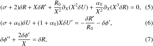$\begin{array}{ccc}& & \mathrm{(}\mathit{\sigma }\mathrm{+}\mathrm{2}\mathrm{)}\mathit{\delta R}\mathrm{+}\mathit{X\delta }{\mathit{R}}^{\mathrm{\prime }}\mathrm{+}\frac{{\mathit{R}}_{\mathrm{0}}}{{\mathit{X}}^{\mathrm{2}}}{\mathit{\partial }}_{\mathit{X}}\mathrm{\left(}{\mathit{X}}^{\mathrm{2}}\mathit{\delta U}\mathrm{\right)}\mathrm{+}\frac{{\mathit{\alpha }}_{\mathrm{0}}}{{\mathit{X}}^{\mathrm{2}}}{\mathit{\partial }}_{\mathit{X}}\mathrm{\left(}{\mathit{X}}^{\mathrm{3}}\mathit{\delta R}\mathrm{\right)}\mathrm{=}\mathrm{0}\mathit{,}\\ & & \mathrm{(}\mathit{\sigma }\mathrm{+}{\mathit{\alpha }}_{\mathrm{0}}\mathrm{)}\mathit{\delta U}\mathrm{+}\mathrm{(}\mathrm{1}\mathrm{+}{\mathit{\alpha }}_{\mathrm{0}}\mathrm{)}\mathit{X\delta }{\mathit{U}}^{\mathrm{\prime }}\mathrm{=}\mathrm{-}\frac{\mathit{\delta }{\mathit{R}}^{\mathrm{\prime }}}{{\mathit{R}}_{\mathrm{0}}}\mathrm{-}\mathit{\delta }{\mathit{\phi }}^{\mathrm{\prime }}\mathit{,}\\ & & \mathit{\delta }{\mathit{\phi }}^{\mathrm{\prime \prime }}\mathrm{+}\frac{\mathrm{2}\mathit{\delta }{\mathit{\phi }}^{\mathrm{\prime }}}{\mathit{X}}\mathrm{=}\mathit{\delta R,}\end{array}$with primes denoting the spatial derivatives. Combining Eqs. (5) and (7), one can show that 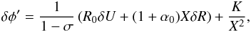$\begin{array}{ccc}\mathit{\delta }{\mathit{\phi }}^{\mathrm{\prime }}\mathrm{=}\frac{\mathrm{1}}{\mathrm{1}\mathrm{-}\mathit{\sigma }}\left({\mathit{R}}_{\mathrm{0}}\mathit{\delta U}\mathrm{+}\mathrm{(}\mathrm{1}\mathrm{+}{\mathit{\alpha }}_{\mathrm{0}}\mathrm{)}\mathit{X\delta R}\right)\mathrm{+}\frac{\mathit{K}}{{\mathit{X}}^{\mathrm{2}}}\mathit{,}& & \end{array}$(8)where K is a constant chosen to ensure the continuity of δφ. From Eqs. (3), (5), (6), we get 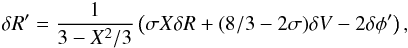$\begin{array}{ccc}\mathit{\delta }{\mathit{R}}^{\mathrm{\prime }}\mathrm{=}\frac{\mathrm{1}}{\mathrm{3}\mathrm{-}{\mathit{X}}^{\mathrm{2}}\mathit{/}\mathrm{3}}\left(\mathit{\sigma X\delta R}\mathrm{+}\mathrm{(}\mathrm{8}\mathit{/}\mathrm{3}\mathrm{-}\mathrm{2}\mathit{\sigma }\mathrm{)}\mathit{\delta V}\mathrm{-}\mathrm{2}\mathit{\delta }{\mathit{\phi }}^{\mathrm{\prime }}\right)\mathit{,}& & \end{array}$(9)which together with Eqs. (6) and (8) allows us to solve the system. Once the boundary conditions have been specified, a numerical integration is carried out by a standard Runge-Kutta scheme.

2.2. Inner boundary and the critical point

The boundary conditions for the perturbation at X ≃ 0 are given by 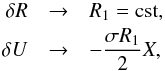$\begin{array}{ccc}\mathit{\delta R}& \mathrm{\to }& {\mathit{R}}_{\mathrm{1}}\mathrm{=}\mathrm{cst}\mathit{,}\\ \mathit{\delta U}& \mathrm{\to }& \mathrm{-}\frac{\mathit{\sigma }{\mathit{R}}_{\mathrm{1}}}{\mathrm{2}}\mathit{X,}\end{array}$(10)where cst is a constant. So by simply specifying a constant value for R₁ we can integrate the system of Eqs. (6) and (8) for different values of σ.

One complication to this otherwise straightforward approach is that the system possesses a critical point at X_crit = 3, where the gas becomes supersonic with respect to the self-similar profile. The presence of such a boundary poses a restriction to our numerical solutions, since only the ones which cross it can be considered physically acceptable.

It is easy to show that the system (5)–(7) has two exact solutions that resemble these boundary conditions and are given by 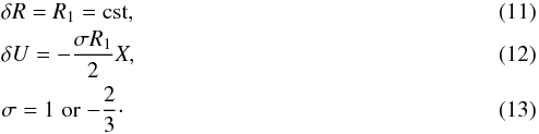$\begin{array}{ccc}& & \mathit{\delta R}\mathrm{=}{\mathit{R}}_{\mathrm{1}}\mathrm{=}\mathrm{cst}\mathit{,}\\ & & \mathit{\delta U}\mathrm{=}\mathrm{-}\frac{\mathit{\sigma }{\mathit{R}}_{\mathrm{1}}}{\mathrm{2}}\mathit{X,}\\ & & \end{array}$While mathematically acceptable, these solutions offer little physical insight: they merely describe a variation of the mean density. They are, however, mathematically acceptable, since they remain small at any X with respect to the perturbed solutions.

Apart from these trivial forms, the integrations of the system of Eqs. (6) and (8) we performed for different values of σ gave no other solutions able to cross the critical point.

2.3. Shock conditions

From the above discussion it becomes clear that a more general form of the perturbation should exist which allows for physically meaningful solutions to the corresponding perturbation equations and which does not suffer from the issue of critical point crossing.

To begin with, one can imagine a core whose size is much larger than the sonic radius. In this case the perturbation can be restricted to the supersonic parts, where X is much greater than the critical value. For a cloud this large we are essentially in the same regime as the cold cloud described by the homologous collapse solution (Eqs. (3)), where gravitational collapse happens before thermal pressure effects have had time to break the self-similarity. We expect then that the behavior of the perturbations will be similar to the general t^-1 growth found by Hunter (1964) for the case of a cold cloud.

In order to integrate the solution for the outer parts of the cloud, we need a physically meaningful boundary condition at the vicinity of the critical point. We thus seek solutions that include a shock. In the vicinity of the critical point, the velocity of the fluid is by definition transonic with respect to the self-similar profile, so an arbitrary weak shock can naturally happen in this area. Note that, although the spatial derivatives of the density and velocity fields are infinite at the shock, all fields remain small if the shock is weak. Therefore, such a discontinuity indeed generates a linear perturbation.

Let the shock be located at X_shock = X_crit + δX where δX> 0. This is the location where the unperturbed solution, given by δR = 0, δU = 0 is connected to a state given by the Rankine-Hugoniot (RH) conditions, which in the frame of reference of the shock are 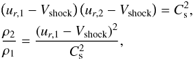$\begin{array}{ccc}& & \left({\mathit{u}}_{\mathit{r,}\mathrm{1}}\mathrm{-}{\mathit{V}}_{\mathrm{shock}}\right)\left({\mathit{u}}_{\mathit{r,}\mathrm{2}}\mathrm{-}{\mathit{V}}_{\mathrm{shock}}\right)\mathrm{=}{\mathit{C}}_{\mathrm{s}}^{\mathrm{2}}\mathit{,}\\ & & \frac{{\mathit{\rho }}_{\mathrm{2}}}{{\mathit{\rho }}_{\mathrm{1}}}\mathrm{=}\frac{\mathrm{(}{\mathit{u}}_{\mathit{r,}\mathrm{1}}\mathrm{-}{\mathit{V}}_{\mathrm{shock}}{\mathrm{)}}^{\mathrm{2}}}{{\mathit{C}}_{\mathrm{s}}^{\mathrm{2}}}\mathit{,}\end{array}$(14)where V_shock is the velocity of the shock and subscripts 1 and 2 mark the pre- and post- shock quantities, respectively.

The velocity of the flow with respect to the self-similar profile is given by α₀X + X = X/ 3. Thus at X_shock, the Mach number can be expressed as ℳ = X_shock/ 3 = 1 + δX/ 3. In the frame of the shock, the gas from the subsonic region is entering supersonically into the shock and therefore constitutes the pre-shock medium whose density is amplified.

Since we consider that the subsonic region is unperturbed, the expressions for ρ₁ and u_r,1 that enter the jump conditions in Eqs. (14) are simply given by Eqs. (2) and (3).

By replacing we get 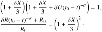$\begin{array}{ccc}& & \left(\mathrm{1}\mathrm{+}\frac{\mathit{\delta X}}{\mathrm{3}}\right)\left(\mathrm{1}\mathrm{+}\frac{\mathit{\delta X}}{\mathrm{3}}\mathrm{+}\mathit{\delta U}\mathrm{(}{\mathit{t}}_{\mathrm{0}}\mathrm{-}\mathit{t}{\mathrm{)}}^{\mathrm{-}\mathit{\sigma }}\right)\mathrm{=}\mathrm{1}\mathit{,}\\ & & \frac{\mathit{\delta R}\mathrm{(}{\mathit{t}}_{\mathrm{0}}\mathrm{-}\mathit{t}{\mathrm{)}}^{\mathrm{-}\mathit{\sigma }}\mathrm{+}{\mathit{R}}_{\mathrm{0}}}{{\mathit{R}}_{\mathrm{0}}}\mathrm{=}{\left(\mathrm{1}\mathrm{+}\frac{\mathit{\delta X}}{\mathrm{3}}\right)}^{\mathrm{2}}\mathrm{·}\end{array}$(15)At the limit of a weak shock, we can expand these relations and get 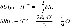$\begin{array}{ccc}& & \mathit{\delta U}\mathrm{(}{\mathit{t}}_{\mathrm{0}}\mathrm{-}\mathit{t}{\mathrm{)}}^{\mathrm{-}\mathit{\sigma }}\mathrm{=}\mathrm{-}\frac{\mathrm{2}}{\mathrm{3}}\mathit{\delta X,}\\ & & \mathit{\delta R}\mathrm{(}{\mathit{t}}_{\mathrm{0}}\mathrm{-}\mathit{t}{\mathrm{)}}^{\mathrm{-}\mathit{\sigma }}\mathrm{=}\frac{\mathrm{2}{\mathit{R}}_{\mathrm{0}}\mathit{\delta X}}{\mathrm{3}}\mathrm{=}\frac{\mathrm{4}}{\mathrm{9}}\mathit{\delta X}\mathit{.}\end{array}$(16)As the perturbation develops it moves toward larger δX, so the density increases and the shock becomes stronger.

Since the perturbed density remains zero up to the position of the shock, the constant K in Eq. (8) must be chosen in such a way that δφ′(X_shock) = 0.

2.4. Limit at large radii

In order to identify the physically relevant solutions, the asymptotic behavior at large X must also been known. From Eqs. (5)–(7), it is easy to infer that there must be an asymptotic behavior of the form 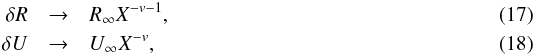$\begin{array}{ccc}\mathit{\delta R}& \mathrm{\to }& {\mathit{R}}_{\mathrm{\infty }}{\mathit{X}}^{\mathrm{-}\mathit{v}\mathrm{-}\mathrm{1}}\mathit{,}\\ \mathit{\delta U}& \mathrm{\to }& {\mathit{U}}_{\mathrm{\infty }}{\mathit{X}}^{\mathrm{-}\mathit{v}}\mathit{,}\end{array}$where the exponent v in Eqs. (17) and (18) should be chosen such that the asymptotic form satisfies Eqs. (5)–(7). By inserting expressions (17) and (18) into Eqs. (5)–(7) and dropping the thermal pressure term, which is negligible at large X, we obtain two linear equations for R_∞ and U_∞, which depend on σ and v. By demanding that the determinant of this system be zero, we get the two solutions for v: $\begin{array}{ccc}\mathit{v}& \mathrm{=}& \mathrm{3}\mathit{\sigma }\mathrm{-}\mathrm{4}\mathit{,}\\ \mathit{v}& \mathrm{=}& \mathrm{3}\mathit{\sigma }\mathrm{+}\mathrm{1.}\end{array}$(19)We thus recover the exact homologous solution mentioned above, since when σ = 1 or −2/3, we get v = −1, which means U ∝ X and R = cst. On closer inspection we also see that the first branch (v = 3σ−4) diverges most rapidly. Since mathematically it is required that v> −1 for the solutions to behave well towards infinity, it follows that σ> 1. When 1 <σ< 4/3, the velocity diverges at infinity but still remains everywhere negligible with respect to the perturbed solution.

2.5. Numerical integration

The shock is now essentially the low-X boundary for the numerical integration, so we only need to specify its position δX from the critical point in order to define the boundary conditions. This value must be small in order to ensure linearity.

As shown by Eqs. (16), the exact values of δU and δR are not important (they depend on t₀, which can be freely chosen) but their ratio is fixed.

Starting from a location close to zero (specifically X_s = 10^-2), and using a step dX = 10^-3, we integrate the perturbation equations up to X = 100. We have checked that the solutions are well resolved and converged.

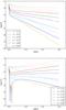Fig. 1 Density (top panel) and velocity (bottom panel) fields of the solutions for various values of σ. For values of X smaller than the position of the shock (X<Xsh ≃ 3), the density and the velocity are unperturbed, i.e. δR = δV = 0. The solid lines show the solutions for the system of Eqs. (5)–(7) For comparison, solutions to the same equations but without the thermal pressure term are shown with the dotted lines.

Figure 1 shows the density and the velocity fields for various values of the growth rate, σ. The solid lines show the solutions of Eqs. (5)–(7) and the dotted lines show the solutions for the same system of equations when the thermal pressure is suppressed. The latter case corresponds to a cold cloud and is given for comparison.

The velocity and the density fields vary rapidly in the vicinity of the shock, X ≃ 3. The velocity, which is negative, increases and the density decreases. At X ≃ 4−5, the behavior of the density changes: it starts decreasing much less rapidly and it quickly reaches the asymptotic behavior expressed by Eqs. (17) and (18).

The behavior of the velocity is slightly more complex. For σ< 4/3, it decreases for X> 4−5 as expected from the asymptotic form (Eqs. (17) and (18)). For 4/3 <σ< 1.6, the velocity eventually decreases and tends towards zero after a small increase. Again, this is in good agreement with the expected asymptotic profile. In contrast, for larger values of σ, the behavior is identical, only the velocity becomes positive just after the shock at X ≃ 3−5, which means that the perturbation is expanding.

Based on this form of the perturbations, we believe that the regime 1 <σ< 4/3 corresponds to the most physically relevant solutions. For smaller σ, the velocity diverges at large X and is therefore not really a perturbation with respect to the unperturbed solution. When σ> 4/3, the velocity quickly tends to zero, meaning that it is very localized around the shock. Finally, when σ> ≃ 1.7, the velocity becomes positive. This situation probably corresponds to somehow artificial perturbations that are unlikely to represent a physically relevant case.

This conclusion remains almost identical for the cold case since for σ< 4/3 the velocity diverges toward large X while for σ> ≃ 1.8, the density becomes negative at X> ≃ 5.

To summarize, we find that linear perturbations that include a weak shock in the vicinity of the sonic point present physically acceptable behavior if the growth rate is larger than unity. As the growth rate becomes larger than 4/3, the form of the eigenvectors suggests that the corresponding perturbation is unlikely to occur: the velocity field rapidly converges toward zero, implying that the perturbation is isolated in the sonic region.

3. Stability analysis: the non-axisymmetric modes

The instability of a shell-like structure is an important result, but if we care about the formation of multiple fragments we must also consider non-spherically shaped perturbations. In this section we present the stability analysis for non-spherically symmetric modes. Since the method is practically the same as the spherical case, here we will only highlight the differences.

3.1. Equations

The fluid equations for a self-gravitating gas in spherical coordinates and three dimensions are: 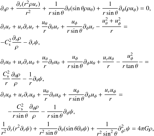$\begin{array}{ccc}& & {\mathit{\partial }}_{\mathit{t}}\mathit{\rho }\mathrm{+}\frac{{\mathit{\partial }}_{\mathit{r}}\mathrm{\left(}{\mathit{r}}^{\mathrm{2}}\mathit{\rho }{\mathit{u}}_{\mathit{r}}\mathrm{\right)}}{{\mathit{r}}^{\mathrm{2}}}\mathrm{+}\frac{\mathrm{1}}{\mathit{r}\sin \mathit{\theta }}{\mathit{\partial }}_{\mathit{\theta }}\mathrm{\left(}\sin \mathit{\theta \rho }{\mathit{u}}_{\mathit{\theta }}\mathrm{\right)}\mathrm{+}\frac{\mathrm{1}}{\mathit{r}\sin \mathit{\theta }}{\mathit{\partial }}_{\mathit{\phi }}\mathrm{\left(}\mathit{\rho }{\mathit{u}}_{\mathit{\phi }}\mathrm{\right)}\mathrm{=}\mathrm{0}\mathit{,}\\ & & {\mathit{\partial }}_{\mathit{t}}{\mathit{u}}_{\mathit{r}}\mathrm{+}{\mathit{u}}_{\mathit{r}}{\mathit{\partial }}_{\mathit{r}}{\mathit{u}}_{\mathit{r}}\mathrm{+}\frac{{\mathit{u}}_{\mathit{\theta }}}{\mathit{r}}{\mathit{\partial }}_{\mathit{\theta }}{\mathit{u}}_{\mathit{r}}\mathrm{+}\frac{{\mathit{u}}_{\mathit{\phi }}}{\mathit{r}\sin \mathit{\theta }}{\mathit{\partial }}_{\mathit{\phi }}{\mathit{u}}_{\mathit{r}}\mathrm{-}\frac{{\mathit{u}}_{\mathit{\theta }}^{\mathrm{2}}\mathrm{+}{\mathit{u}}_{\mathit{\phi }}^{\mathrm{2}}}{\mathit{r}}\mathrm{=}\\ & & \mathrm{-}{\mathit{C}}_{\mathrm{s}}^{\mathrm{2}}\frac{{\mathit{\partial }}_{\mathit{r}}\mathit{\rho }}{\mathit{\rho }}\mathrm{-}{\mathit{\partial }}_{\mathit{r}}\mathit{\psi ,}\\ & & {\mathit{\partial }}_{\mathit{t}}{\mathit{u}}_{\mathit{\theta }}\mathrm{+}{\mathit{u}}_{\mathit{r}}{\mathit{\partial }}_{\mathit{r}}{\mathit{u}}_{\mathit{\theta }}\mathrm{+}\frac{{\mathit{u}}_{\mathit{\theta }}}{\mathit{r}}{\mathit{\partial }}_{\mathit{\theta }}{\mathit{u}}_{\mathit{\theta }}\mathrm{+}\frac{{\mathit{u}}_{\mathit{\phi }}}{\mathit{r}\sin \mathit{\theta }}{\mathit{\partial }}_{\mathit{\phi }}{\mathit{u}}_{\mathit{\theta }}\mathrm{+}\frac{{\mathit{u}}_{\mathit{r}}{\mathit{u}}_{\mathit{\theta }}}{\mathit{r}}\mathrm{-}\frac{{\mathit{u}}_{\mathit{\phi }}^{\mathrm{2}}}{\mathit{r}\tan \mathit{\theta }}\mathrm{-}\mathrm{=}\\ & & \frac{{\mathit{C}}_{\mathrm{s}}^{\mathrm{2}}}{\mathit{r}}\frac{{\mathit{\partial }}_{\mathit{\theta }}\mathit{\rho }}{\mathit{\rho }}\mathrm{-}\frac{\mathrm{1}}{\mathit{r}}{\mathit{\partial }}_{\mathit{\theta }}\mathit{\psi ,}\\ & & {\mathit{\partial }}_{\mathit{t}}{\mathit{u}}_{\mathit{\phi }}\mathrm{+}{\mathit{u}}_{\mathit{r}}{\mathit{\partial }}_{\mathit{r}}{\mathit{u}}_{\mathit{\phi }}\mathrm{+}\frac{{\mathit{u}}_{\mathit{\theta }}}{\mathit{r}}{\mathit{\partial }}_{\mathit{\theta }}{\mathit{u}}_{\mathit{\phi }}\mathrm{+}\frac{{\mathit{u}}_{\mathit{\phi }}}{\mathit{r}\sin \mathit{\theta }}{\mathit{\partial }}_{\mathit{\phi }}{\mathit{u}}_{\mathit{\phi }}\mathrm{+}\frac{{\mathit{u}}_{\mathit{r}}{\mathit{u}}_{\mathit{\phi }}}{\mathit{r}}\mathrm{=}\\ & & \mathrm{-}\frac{{\mathit{C}}_{\mathrm{s}}^{\mathrm{2}}}{\mathit{r}\sin \mathit{\theta }}\frac{{\mathit{\partial }}_{\mathit{\phi }}\mathit{\rho }}{\mathit{\rho }}\mathrm{-}\frac{\mathrm{1}}{\mathit{r}\sin \mathit{\theta }}{\mathit{\partial }}_{\mathit{\phi }}\mathit{\psi ,}\\ & & \frac{\mathrm{1}}{{\mathit{r}}^{\mathrm{2}}}{\mathit{\partial }}_{\mathit{r}}\mathrm{\left(}{\mathit{r}}^{\mathrm{2}}{\mathit{\partial }}_{\mathit{r}}\mathit{\psi }\mathrm{\right)}\mathrm{+}\frac{\mathrm{1}}{{\mathit{r}}^{\mathrm{2}}\sin \mathit{\theta }}{\mathit{\partial }}_{\mathit{\theta }}\mathrm{\left(}\sin \mathit{\theta }{\mathit{\partial }}_{\mathit{\theta }}\mathit{\psi }\mathrm{\right)}\mathrm{+}\frac{\mathrm{1}}{{\mathit{r}}^{\mathrm{2}}{\sin }^{\mathrm{2}}\mathit{\theta }}{\mathit{\partial }}_{{\mathit{\phi }}^{\mathrm{2}}}^{\mathrm{2}}\mathit{\psi }\mathrm{=}\mathrm{4}\mathit{\pi G\rho ,}\end{array}$(20)where u_r, u_θ, and u_φ denote the velocities along each of the spherical coordinates r, θ and φ. To study the stability of the homologous solution with respect to non-spherical modes, we look for perturbations of the form (HM99): 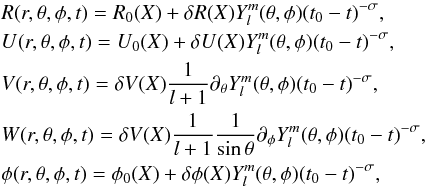$\begin{array}{ccc}& & \mathit{R}\mathrm{\left(}\mathit{r,\theta ,\phi ,t}\mathrm{\right)}\mathrm{=}{\mathit{R}}_{\mathrm{0}}\mathrm{\left(}\mathit{X}\mathrm{\right)}\mathrm{+}\mathit{\delta R}\mathrm{\left(}\mathit{X}\mathrm{\right)}{\mathit{Y}}_{\mathit{l}}^{\mathit{m}}\mathrm{\left(}\mathit{\theta ,\phi }\mathrm{\right)}\mathrm{(}{\mathit{t}}_{\mathrm{0}}\mathrm{-}\mathit{t}{\mathrm{)}}^{\mathrm{-}\mathit{\sigma }}\mathit{,}\\ & & \mathit{U}\mathrm{\left(}\mathit{r,\theta ,\phi ,t}\mathrm{\right)}\mathrm{=}{\mathit{U}}_{\mathrm{0}}\mathrm{\left(}\mathit{X}\mathrm{\right)}\mathrm{+}\mathit{\delta U}\mathrm{\left(}\mathit{X}\mathrm{\right)}{\mathit{Y}}_{\mathit{l}}^{\mathit{m}}\mathrm{\left(}\mathit{\theta ,\phi }\mathrm{\right)}\mathrm{(}{\mathit{t}}_{\mathrm{0}}\mathrm{-}\mathit{t}{\mathrm{)}}^{\mathrm{-}\mathit{\sigma }}\mathit{,}\\ & & \mathit{V}\mathrm{\left(}\mathit{r,\theta ,\phi ,t}\mathrm{\right)}\mathrm{=}\mathit{\delta V}\mathrm{\left(}\mathit{X}\mathrm{\right)}\frac{\mathrm{1}}{\mathit{l}\mathrm{+}\mathrm{1}}{\mathit{\partial }}_{\mathit{\theta }}{\mathit{Y}}_{\mathit{l}}^{\mathit{m}}\mathrm{\left(}\mathit{\theta ,\phi }\mathrm{\right)}\mathrm{(}{\mathit{t}}_{\mathrm{0}}\mathrm{-}\mathit{t}{\mathrm{)}}^{\mathrm{-}\mathit{\sigma }}\mathit{,}\\ & & \mathit{W}\mathrm{\left(}\mathit{r,\theta ,\phi ,t}\mathrm{\right)}\mathrm{=}\mathit{\delta V}\mathrm{\left(}\mathit{X}\mathrm{\right)}\frac{\mathrm{1}}{\mathit{l}\mathrm{+}\mathrm{1}}\frac{\mathrm{1}}{\sin \mathit{\theta }}{\mathit{\partial }}_{\mathit{\phi }}{\mathit{Y}}_{\mathit{l}}^{\mathit{m}}\mathrm{\left(}\mathit{\theta ,\phi }\mathrm{\right)}\mathrm{(}{\mathit{t}}_{\mathrm{0}}\mathrm{-}\mathit{t}{\mathrm{)}}^{\mathrm{-}\mathit{\sigma }}\mathit{,}\\ & & \mathit{\phi }\mathrm{\left(}\mathit{r,\theta ,\phi ,t}\mathrm{\right)}\mathrm{=}{\mathit{\phi }}_{\mathrm{0}}\mathrm{\left(}\mathit{X}\mathrm{\right)}\mathrm{+}\mathit{\delta \phi }\mathrm{\left(}\mathit{X}\mathrm{\right)}{\mathit{Y}}_{\mathit{l}}^{\mathit{m}}\mathrm{\left(}\mathit{\theta ,\phi }\mathrm{\right)}\mathrm{(}{\mathit{t}}_{\mathrm{0}}\mathrm{-}\mathit{t}{\mathrm{)}}^{\mathrm{-}\mathit{\sigma }}\mathit{,}\end{array}$(21)where V and W are the angular velocities and δV(X), δW(X) are the corresponding perturbations in the self-similar frame and ${\mathit{Y}}_{\mathit{l}}^{\mathit{m}}\mathrm{\left(}\mathit{\theta ,\phi }\mathrm{\right)}$ are the usual spherical harmonics. As in the study of HM99, the equations for δV and δW are identical so the perturbations are given the same amplitude, δV(X). Replacing these expressions into Eqs. (20), we get 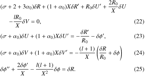$\begin{array}{ccc}& & \mathrm{(}\mathit{\sigma }\mathrm{+}\mathrm{2}\mathrm{+}\mathrm{3}{\mathit{\alpha }}_{\mathrm{0}}\mathrm{)}\mathit{\delta R}\mathrm{+}\mathrm{(}\mathrm{1}\mathrm{+}{\mathit{\alpha }}_{\mathrm{0}}\mathrm{)}\mathit{X\delta }{\mathit{R}}^{\mathrm{\prime }}\mathrm{+}{\mathit{R}}_{\mathrm{0}}\mathit{\delta }{\mathit{U}}^{\mathrm{\prime }}\mathrm{+}\frac{\mathrm{2}{\mathit{R}}_{\mathrm{0}}}{\mathit{X}}\mathit{\delta U}\\ & & \mathrm{-}\frac{\mathit{l}{\mathit{R}}_{\mathrm{0}}}{\mathit{X}}\mathit{\delta V}\mathrm{=}\mathrm{0}\mathit{,}\\ & & \mathrm{(}\mathit{\sigma }\mathrm{+}{\mathit{\alpha }}_{\mathrm{0}}\mathrm{)}\mathit{\delta U}\mathrm{+}\mathrm{(}\mathrm{1}\mathrm{+}{\mathit{\alpha }}_{\mathrm{0}}\mathrm{)}\mathit{X\delta }{\mathit{U}}^{\mathrm{\prime }}\mathrm{=}\mathrm{-}\frac{\mathit{\delta }{\mathit{R}}^{\mathrm{\prime }}}{{\mathit{R}}_{\mathrm{0}}}\mathrm{-}\mathit{\delta }{\mathit{\phi }}^{\mathrm{\prime }}\mathit{,}\\ & & \mathrm{(}\mathit{\sigma }\mathrm{+}{\mathit{\alpha }}_{\mathrm{0}}\mathrm{)}\mathit{\delta V}\mathrm{+}\mathrm{(}\mathrm{1}\mathrm{+}{\mathit{\alpha }}_{\mathrm{0}}\mathrm{)}\mathit{X\delta }{\mathit{V}}^{\mathrm{\prime }}\mathrm{=}\mathrm{-}\frac{\mathrm{(}\mathit{l}\mathrm{+}\mathrm{1}\mathrm{)}}{\mathit{X}}\left(\frac{\mathit{\delta R}}{{\mathit{R}}_{\mathrm{0}}}\mathrm{+}\mathit{\delta \phi }\right)\\ & & \mathit{\delta }{\mathit{\phi }}^{\mathrm{\prime \prime }}\mathrm{+}\frac{\mathrm{2}\mathit{\delta }{\mathit{\phi }}^{\mathrm{\prime }}}{\mathit{X}}\mathrm{-}\frac{\mathit{l}\mathrm{(}\mathit{l}\mathrm{+}\mathrm{1}\mathrm{)}}{{\mathit{X}}^{\mathrm{2}}}\mathit{\delta \phi }\mathrm{=}\mathit{\delta R}\mathit{.}\end{array}$Thus, the system of Eqs. (22)–(25) consists of three first-order ordinary differential equations and one second-order ordinary differential equation. Like in the spherical case, we solve it using a standard Runge-Kutta method.

3.2. Inner boundary and shock condition in the non-axisymmetric case

The boundary conditions of Eqs. (22)–(25) at X ≃ 0 are given by 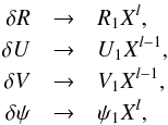$\begin{array}{ccc}\mathit{\delta R}& \mathrm{\to }& {\mathit{R}}_{\mathrm{1}}{\mathit{X}}^{\mathit{l}}\mathit{,}\\ \mathit{\delta U}& \mathrm{\to }& {\mathit{U}}_{\mathrm{1}}{\mathit{X}}^{\mathit{l}\mathrm{-}\mathrm{1}}\mathit{,}\\ \mathit{\delta V}& \mathrm{\to }& {\mathit{V}}_{\mathrm{1}}{\mathit{X}}^{\mathit{l}\mathrm{-}\mathrm{1}}\mathit{,}\\ \mathit{\delta \psi }& \mathrm{\to }& {\mathit{\psi }}_{\mathrm{1}}{\mathit{X}}^{\mathit{l}}\mathit{,}\end{array}$(26)where 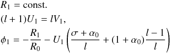$\begin{array}{ccc}& & {\mathit{R}}_{\mathrm{1}}\mathrm{=}\mathrm{const}\mathit{.}\\ & & \mathrm{(}\mathit{l}\mathrm{+}\mathrm{1}\mathrm{)}{\mathit{U}}_{\mathrm{1}}\mathrm{=}\mathit{l}{\mathit{V}}_{\mathrm{1}}\mathit{,}\\ & & {\mathit{\phi }}_{\mathrm{1}}\mathrm{=}\mathrm{-}\frac{{\mathit{R}}_{\mathrm{1}}}{{\mathit{R}}_{\mathrm{0}}}\mathrm{-}{\mathit{U}}_{\mathrm{1}}\left(\frac{\mathit{\sigma }\mathrm{+}{\mathit{\alpha }}_{\mathrm{0}}}{\mathit{l}}\mathrm{+}\mathrm{(}\mathrm{1}\mathrm{+}{\mathit{\alpha }}_{\mathrm{0}}\mathrm{)}\frac{\mathit{l}\mathrm{-}\mathrm{1}}{\mathit{l}}\right)\end{array}$(27)for the system to have a solution. Equations (22)–(25) admit a family of solutions that resemble these boundary conditions and are given by Eqs. (26) and 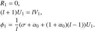$\begin{array}{ccc}& & {\mathit{R}}_{\mathrm{1}}\mathrm{=}\mathrm{0}\mathit{,}\\ & & \mathrm{(}\mathit{l}\mathrm{+}\mathrm{1}\mathrm{)}{\mathit{U}}_{\mathrm{1}}\mathrm{=}\mathit{l}{\mathit{V}}_{\mathrm{1}}\mathit{,}\\ & & {\mathit{\phi }}_{\mathrm{1}}\mathrm{=}\frac{\mathrm{1}}{\mathit{l}}\mathrm{(}\mathit{\sigma }\mathrm{+}{\mathit{\alpha }}_{\mathrm{0}}\mathrm{+}\mathrm{(}\mathrm{1}\mathrm{+}{\mathit{\alpha }}_{\mathrm{0}}\mathrm{\left)}\mathrm{\right(}\mathit{l}\mathrm{-}\mathrm{1}\mathrm{\left)}\mathrm{\right)}{\mathit{U}}_{\mathrm{1}}\mathit{.}\end{array}$(28)The situation here resembles what we found for the spherical problem: while these solutions are mathematically acceptable, they diverge at large X so they do not represent physical solutions. Nonetheless, they will play an important role in finding a solution, as we will show later.

It is easy to see that this system also admits a critical point located at X_crit = 3. Again, the only solutions that satisfy the inner boundary conditions and cross the critical point are the trivial ones stated by Eqs. (28), which for l> 2 diverge at infinity.

Following the same line of thought, we look for solutions that present a shock at the vicinity of the critical point, X_shock = X_crit + δX where δX> 0. The unperturbed solution given by δR = 0, δU = 0 is connected to a post-shock state given by the Rankine-Hugoniot conditions. The same applies to the other variables δV, δφ and δφ′. They are all assumed to be zero in the inner part before the shock. These variables however are continuous so they are also equal to zero immediately after the shock.

The Rankine-Hugoniot conditions are identical to the spherical case. The same calculations then lead to 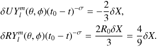$\begin{array}{ccc}& & \mathit{\delta U}{\mathit{Y}}_{\mathit{l}}^{\mathit{m}}\mathrm{\left(}\mathit{\theta ,\phi }\mathrm{\right)}\mathrm{(}{\mathit{t}}_{\mathrm{0}}\mathrm{-}\mathit{t}{\mathrm{)}}^{\mathrm{-}\mathit{\sigma }}\mathrm{=}\mathrm{-}\frac{\mathrm{2}}{\mathrm{3}}\mathit{\delta X,}\\ & & \mathit{\delta R}{\mathit{Y}}_{\mathit{l}}^{\mathit{m}}\mathrm{\left(}\mathit{\theta ,\phi }\mathrm{\right)}\mathrm{(}{\mathit{t}}_{\mathrm{0}}\mathrm{-}\mathit{t}{\mathrm{)}}^{\mathrm{-}\mathit{\sigma }}\mathrm{=}\frac{\mathrm{2}{\mathit{R}}_{\mathrm{0}}\mathit{\delta X}}{\mathrm{3}}\mathrm{=}\frac{\mathrm{4}}{\mathrm{9}}\mathit{\delta X}\mathit{.}\end{array}$(29)This implies that the surface of the shock itself is spherical only at the zeroth order. At the first order, the shock surface is described by a spherical harmonic, ${\mathit{Y}}_{\mathit{l}}^{\mathit{m}}$.

3.3. Limit at large radii for non-axisymmetric modes

From Eqs. (22)–(25), it is easy to infer that the asymptotic behavior towards infinity is 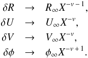$\begin{array}{ccc}\mathit{\delta R}& \mathrm{\to }& {\mathit{R}}_{\mathrm{\infty }}{\mathit{X}}^{\mathrm{-}\mathit{v}\hspace{0.17em}\mathrm{-}\hspace{0.17em}\mathrm{1}}\mathit{,}\\ \mathit{\delta U}& \mathrm{\to }& {\mathit{U}}_{\mathrm{\infty }}{\mathit{X}}^{\mathrm{-}\mathit{v}}\mathit{,}\\ \mathit{\delta V}& \mathrm{\to }& {\mathit{V}}_{\mathrm{\infty }}{\mathit{X}}^{\mathrm{-}\mathit{v}}\mathit{,}\\ \mathit{\delta \phi }& \mathrm{\to }& {\mathit{\phi }}_{\mathrm{\infty }}{\mathit{X}}^{\mathrm{-}\mathit{v}\hspace{0.17em}\mathrm{+}\hspace{0.17em}\mathrm{1}}\mathit{.}\end{array}$(30)By inserting these expressions into Eqs. (22)–(25) we obtain a fourth-order polynomial whose four roots are: 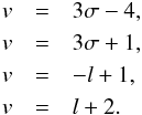$\begin{array}{ccc}\mathit{v}& \mathrm{=}& \mathrm{3}\mathit{\sigma }\mathrm{-}\mathrm{4}\mathit{,}\\ \mathit{v}& \mathrm{=}& \mathrm{3}\mathit{\sigma }\mathrm{+}\mathrm{1}\mathit{,}\\ \mathit{v}& \mathrm{=}& \mathrm{-}\mathit{l}\mathrm{+}\mathrm{1}\mathit{,}\\ \mathit{v}& \mathrm{=}& \mathit{l}\mathrm{+}\mathrm{2.}\end{array}$(31)The two first roots are the same ones we obtained before. The third branch, v = −l + 1, leads to a strong divergence with l, with the exception of the value l = 2 for which it leads to the same asymptotic behavior as the solution stated by Eqs. (3). This asymptotic form is associated to the solution stated by Eqs. (28) and it is, generally speaking, unphysical.

However, if this branch is linearly combined with the solution (28) in such a way that their asymptotic behaviors compensate, the new solution can be made to present a physically acceptable asymptotic behavior described by the root v = 3σ−4, like in the spherical case. It is again required that v> −1, so we must have σ> 1. Also, the condition that the velocity go to 0 at large X implies again that σ> 4/3.

To summarize, in order to get physically meaningful perturbations of the exact solution stated by Eqs. (3), we need to combine the solution stated by Eqs. (28) with the solution obtained by applying the Rankine-Hugoniot conditions at the vicinity of the critical point in such a way that the linear combination does not diverge too strongly.

If S_l is the desired solution and φ₁ is the value of the linear combination in Eqs. (28), then before the shock the solution is given by Eqs. (26) and (28). At the shock position the solution must satisfy the jump relations stated by Eqs. (29). The difference with the spherical case is that here u_r,1 is not zero, but given by Eqs. (28). This leads to $\begin{array}{ccc}\mathit{\delta U}{\mathit{Y}}_{\mathit{l}}^{\mathit{m}}\mathrm{(}{\mathit{t}}_{\mathrm{0}}\mathrm{-}\mathit{t}{\mathrm{)}}^{\mathrm{-}\mathit{\sigma }}& \mathrm{=}& \mathrm{-}\frac{\mathrm{2}}{\mathrm{3}}\mathit{\delta X}\mathrm{-}{\mathit{U}}_{\mathrm{1}}{\mathit{X}}_{\mathrm{shock}}^{\mathit{l}\hspace{0.17em}\mathrm{-}\hspace{0.17em}\mathrm{1}}{\mathit{Y}}_{\mathit{l}}^{\mathit{m}}\mathrm{(}{\mathit{t}}_{\mathrm{0}}\mathrm{-}\mathit{t}{\mathrm{)}}^{\mathrm{-}\mathit{\sigma }}\mathit{,}\\ \mathit{\delta R}{\mathit{Y}}_{\mathit{l}}^{\mathit{m}}\mathrm{(}{\mathit{t}}_{\mathrm{0}}\mathrm{-}\mathit{t}{\mathrm{)}}^{\mathrm{-}\mathit{\sigma }}& \mathrm{=}& \mathrm{2}{\mathit{R}}_{\mathrm{0}}\left(\frac{\mathit{\delta X}}{\mathrm{3}}\mathrm{+}{\mathit{U}}_{\mathrm{1}}{\mathit{X}}_{\mathrm{shock}}^{\mathit{l}\hspace{0.17em}\mathrm{-}\hspace{0.17em}\mathrm{1}}{\mathit{Y}}_{\mathit{l}}^{\mathit{m}}\mathrm{(}{\mathit{t}}_{\mathrm{0}}\mathrm{-}\mathit{t}{\mathrm{)}}^{\mathrm{-}\mathit{\sigma }}\right)\mathit{,}\end{array}$(32)while $\begin{array}{ccc}\mathit{\delta V}& \mathrm{=}& {\mathit{V}}_{\mathrm{1}}{\mathit{X}}_{\mathrm{shock}}^{\mathit{l}\hspace{0.17em}\mathrm{-}\hspace{0.17em}\mathrm{1}}\mathit{,}\\ \mathit{\delta \phi }& \mathrm{=}& {\mathit{\phi }}_{\mathrm{1}}{\mathit{X}}_{\mathrm{shock}}^{\mathit{l}\mathrm{+}\mathrm{1}}{\mathit{Y}}_{\mathit{l}}^{\mathit{m}}\mathit{.}\end{array}$(33)Thus S_l is a linear combination of the two above solutions. This is made clearer by writing $\begin{array}{ccc}\mathit{\delta U}{\mathit{Y}}_{\mathit{l}}^{\mathit{m}}\mathrm{(}{\mathit{t}}_{\mathrm{0}}\mathrm{-}\mathit{t}{\mathrm{)}}^{\mathrm{-}\mathit{\sigma }}& \mathrm{=}& \mathrm{-}\frac{\mathrm{2}}{\mathrm{3}}\mathit{\delta }{\mathit{X}}^{\mathrm{\prime }}\mathrm{+}{\mathit{U}}_{\mathrm{1}}{\mathit{X}}_{\mathrm{shock}}^{\mathit{l}\mathrm{-}\mathrm{1}}{\mathit{Y}}_{\mathit{l}}^{\mathit{m}}\mathrm{(}{\mathit{t}}_{\mathrm{0}}\mathrm{-}\mathit{t}{\mathrm{)}}^{\mathrm{-}\mathit{\sigma }}\mathit{,}\\ \mathit{\delta R}{\mathit{Y}}_{\mathit{l}}^{\mathit{m}}\mathrm{(}{\mathit{t}}_{\mathrm{0}}\mathrm{-}\mathit{t}{\mathrm{)}}^{\mathrm{-}\mathit{\sigma }}& \mathrm{=}& \frac{\mathrm{2}{\mathit{R}}_{\mathrm{0}}}{\mathrm{3}}\mathit{\delta }{\mathit{X}}^{\mathrm{\prime }}\mathit{,}\end{array}$(34)where $\mathit{\delta }{\mathit{X}}^{\mathrm{\prime }}\mathrm{=}\mathit{\delta X}\mathrm{+}{\mathit{U}}_{\mathrm{1}}{\mathit{X}}_{\mathrm{shock}}^{\mathit{l}\mathrm{-}\mathrm{1}}{\mathit{Y}}_{\mathit{l}}^{\mathit{m}}\mathrm{(}{\mathit{t}}_{\mathrm{0}}\mathrm{-}\mathit{t}{\mathrm{)}}^{\mathit{\sigma }}$. We see that the first terms of the right-hand side of Eqs. (34) are identical to Eqs. (29), while the second terms are compatible with Eqs. (28).

It is interesting that, unlike in the spherically symmetric problem, here the perturbations cannot vanish in the subsonic region. Since gravity is a non-local force, these perturbations are induced inside the subsonic region by the non-axisymmetric density distribution of the supersonic region.

Strictly speaking, since the spherical harmonics ${\mathit{Y}}_{\mathit{m}}^{\mathit{l}}$ also take negative values, there are locations where expressions (29) and (34) place the shock in the subsonic regions of the core. In order for the shock to always be outside the critical point or, in other words, in order for δX to always be positive, these expressions should contain a spherically symmetric term. This can be achieved by combining the non-axisymmetric perturbations with the spherically symmetric perturbation described by Eq. (13) for σ = 1, so essentially adding an extra term, constant in (θ, φ), in Eqs. (29)–(34) that describe the Rankine-Hugoniot conditions. We have omitted such a term for the sake of simplicity, but the subsequent analysis would remain identical. Indeed, we have verified that the solutions depend only weakly on the inner boundary conditions.

3.4. Results for the non-axisymmetric modes

As in the spherical case, here as well we specify a position for the shock δX small enough to ensure linearity. We use a step dX = 10^-3 and integrate up to X = 10⁴. At the high X limit we divide the potential by X^{l + 1}, which yields the parameter φ₁ (see Eq. (33)). To obtain S_l then we subtract the unphysical solution (28) from the result of the numerical integration and recover the expected asymptotic behavior for values of X smaller than 10⁴. An artifact of this subtraction is that, when X ≃ 10⁴ the potential goes abruptly to zero. The integration to larger values of X compared to the spherical problem enables us to discard the diverging term while maintaining a physical behavior for a large enough range of X values.

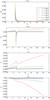Fig. 2 From top to bottom, density R, radial velocity U, azimuthal velocity V and gravitational potential φ for the l = 2 mode and for a series of growth rates.

Fig. 3 Same as Fig. 2 for the l = 3 mode.

Fig. 4 Same as Fig. 2 for the l = 4 mode.

Figures 2–4 show the density R, radial and azimuthal velocities U and V and the gravitational potential φ for the azimuthal wave numbers l = 2, 3 and 4 respectively and for a series of growth rates σ. These profiles show the solutions described by Eqs. (28) in the inner subsonic regions, then a shock in the neighborhood of the critical point X_c ≃ 3 and finally a behavior at large X consistent with the asymptotic analysis above and similar to the spherically symmetric case.

Although not identical, the three modes behave similarly to the spherically symmetric example. The values of the various fields tend to be smaller for larger l because the gravitational potential has stiffer spatial variations in the azimuthal directions, which lowers the resulting force inside the subsonic regions. Like in the simple one-dimensional case, here as well higher values of σ lead to sharply peaked profiles around the shock position. This appears to suggest that the physically relevant values of σ are between 1 and ≃1.5, but at the same time, there does not seem to be an obvious way of deciding whether a particular growth rate is expected or preferred. For this reason and also for the sake of verifying the reliability of the present approach, we perform numerical simulations, which are presented in the following section.

4. Stability of collapsing cores in numerical simulations

The above analysis is complemented with a series of numerical experiments, consisting of collapsing cores with different initial ratios of gravitational to thermal energy (virial parameter α), and different initial perturbations. These simulations are a very efficient way to witness the behavior of a linearly perturbed core in the full complexity that three-dimensionality entails, meaning the inclusion of the azimuthal and vertical velocity components. It also allows us to probe the limit for fragmentation as the thermal support of the core increases.

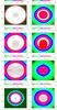Fig. 5 Contours of the log  nH in units of mH cm-3 along the yz plane. From top to bottom: l = 0, l = 1, l = 2 and l = 3 modes for virial parameter α = 0.006. The units along each axis are parsecs and tff stands for free-fall time.

4.1. Code and initial conditions

The simulations are performed with the publicly available Adaptive Mesh Refinement (AMR) code RAMSES (Teyssier 2002), which solves the equations of hydrodynamics on a Cartesian grid with a second-order Godunov scheme and comes with wide range of options for the simulated physical processes. In this case we take advantage of its AMR capabilities by requiring that the Jeans length be always resolved with at least 20 grid cells. An isothermal equation of state is used throughout.

The initial condition of each simulation is a core of uniform density ρ₀, equal to 4 × 10^-18 g cm^-3, and uniform temperature T, equal to 10 K. To this profile we add a linear perturbation, given by $\begin{array}{ccc}\mathit{\delta \rho }\mathrm{=}\mathrm{[}{\mathit{ϵ}}_{\mathrm{1}}\cos \mathrm{(}{\mathit{k}}_{\mathit{r}}\mathrm{·}\mathrm{2}\mathit{\pi r}\mathit{/}{\mathit{L}}_{\mathrm{c}}\mathrm{)}\mathrm{·}\mathrm{(}\mathrm{1}\mathrm{+}{\mathit{ϵ}}_{\mathrm{2}}{\mathit{Y}}_{\mathit{l}}^{\mathit{m}}\mathrm{(}\mathit{\theta ,\phi }{\mathrm{)}}^{\mathrm{]}}& & \end{array}$(35)where k_r = 0.25 is the radial wavenumber of the perturbation, r is the distance from the core center, L_c is the core outer radius and ϵ₁, ϵ₂ the amplitudes of each component of the perturbation, which, according to the case, have values from 0.05 to 0.1. The core resides in a uniform medium of pressure and density 100 times smaller than the core’s interior.

For all these simulations we employ periodic boundary conditions; when self-gravity is involved, such boundaries can potentially affect the evolution of the system, so the core is placed at the center of the computational volume, at a distance of two core radii from each box side. This was shown to be enough to avoid boundary effects by convergence tests we performed for the largest core.

4.2. Stability as a function of cloud parameters

In this study of the core stability, we vary only two parameters: the azimuthal wave number l of the spherical harmonics and the virial parameter of the core, which gives the thermal over gravitational energy ratio in the core and is defined as 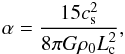$\begin{array}{ccc}\mathit{\alpha }\mathrm{=}\frac{\mathrm{15}{\mathit{c}}_{\mathrm{s}}^{\mathrm{2}}}{\mathrm{8}\mathit{\pi G}{\mathit{\rho }}_{\mathrm{0}}{\mathit{L}}_{\mathrm{c}}^{\mathrm{2}}}\mathit{,}& & \end{array}$(36)where c_s is the sound speed in the core interior. Here the temperature of the core is held constant and α is varied by changing the radius R of the core. We have not varied the radial wavenumber of the perturbation, which means the l = 0 case is a single shell around the center of the core.

Some examples of the core behavior are shown in Figs. 5 and 6, where we show density contour plots of a cut along the yz plane in the middle of the simulation box for different times of each simulation. For low virial parameters (largest cores, α< 0.15) the density peaks are more and more enhanced with respect to the background, which, as the collapse continues, can lead to the formation of as many objects as the peaks of the initial perturbation. In the intermediate virial parameter regime (0.15 <α< 0.6), the perturbations are erased by the expanding rarefaction wave and the core collapses into one single fragment. In the large virial parameter regime (0.6 <α, smallest cores) the core is no longer held by gravity and re-expands under the influence of its thermal pressure.

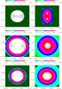Fig. 6 Contours of the log nH in units of mH cm-3 along the yz plane. From top to bottom: l = 2 mode for virial parameters α = 0.1, α = 0.2 and α = 0.8. Like in Fig. 5, units along each axis are parsecs and tff stands for free-fall time.

4.3. Growth rates

The growth rate of the initial perturbation is measured as the rate of change of δρ/ρ₀, where δρ = ρ_max − ρ₀. Here ρ_max is defined as the maximum density in the core and ρ₀ as the central density of the core at each instant. The time is normalized as t′ = 1 − t/t_ff, where t the actual time in the simulation and t_ff the initial free-fall time of the core, t_ff = 3π/32Gρ₀, where ρ₀ the initial density of the core. In practice, we plot the logarithm of these quantities and calculate a least-square fit to the linear regime of the plot. The slope of this fit is the negative of the growth rate we are after. To make it clearer, if the denote the growth rate with σ, like in the analytical treatment of the previous sections, then ⁽δR/R₀⁾ = ⁽δR/R₀⁾₀t^′σ (see Eq. (4) for the definition of the quantities, with the exception of t′, which here denotes the simulation time). By taking the logarithm of this relation one can clearly see that σ becomes the slope of a linear relation between log ⁽δR/R₀⁾ and log  (t′). But since in our notation time is negative, we must also take the negative of the slope as the growth rate of the instability.

Some growth rates thus calculated are shown plotted in Figs. 7–9.

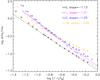Fig. 7 Growth rates for α = 0.006 mode for azimuthal wave numbers l.

Following a simple line of thought, we expect the highest growth rates to appear for the smallest l, since the azimuthal flow of material is then focused on a smaller number of fragments, which can therefore grow faster. At the limit of very high l on the other hand, one expects to recover σ values similar to the l = 0 case, since a very large number of fragments in the azimuthal direction is roughly equivalent to a continuous shell structure.

Figure 7 shows the growth rates for the case of the largest core, with a virial parameter of α = 0.006. For the low-l regime (approximately 0 <l< 10), the growth rates inferred from the simulations are above the value of 1, in excellent agreement with the analytical prediction of the previous sections. Also, the highest growth rates are observed for l = 1 and l = 2, in accordance with the simple prediction just above. But for very high values of l, instead of tending towards the value of σ for l = 0 the growth rates in the simulations fall below unity. This disagreement can probably be attributed to a lack of angular resolution.

Figures 8 and 9 show growth rates for the same azimuthal wavenumber (l = 0 and l = 2, respectively), but for different virial parameters α. Both figures show a similar pattern: a decrease in the growth rate as the virial parameter increases, which can be understood as an increasing thermal stability of the core. As thermal pressure becomes important, the rarefaction wave is increasingly more efficient in weakening the perturbation, to the point that, for large enough α, it does not grow anymore.

At this point we should mention that it was impossible to locate the weak shock in the simulations, due to the very limited resolution in the central parts of the core (the region with X< 3 was only resolved with three to five cells). This makes a direct comparison of the eigenvectors very challenging. Nonetheless, the excellent agreement of the growth rates obtained with two such different methods is very encouraging.

5. Discussion and implications

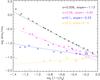Fig. 8 Growth rates of the l = 0 mode for various virial parameters α.

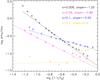Fig. 9 Growth rates of the l = 2 mode for various virial parameters α.

The most important result of the present work is that a homologously collapsing cloud is prone to a shell instability due to its self-gravity, even for non-axisymmetric perturbations with large azimuthal wave numbers. This instability develops relatively fast when the cloud has little thermal support, showing growth rates typically larger than 1 and up to 1.2–1.3 for l = 2. These growth rates decrease when the thermal support increases and eventually reach zero, meaning that the cloud is not expected to undergo fragmentation, at least not through the shell-like mode studied here.

It is important to contrast this result with the analysis of HM99 for the LP solution. In their study, only the l = 2 mode is unstable and it grows like ≃(t₀ − t)^-0.354. Since the density ρ is proportional to (t₀ − t)^-2, this implies that the perturbation grows like ≃ρ^0.175. Therefore, a perturbation starting with an amplitude ϵ ≃ 0.1 should become nonlinear (ϵ ≃ 1), only when the density within the cloud has grown by 10^1/0.175 ≃ 5 × 10⁵. This is such a significant density increase that this instability may never happen. Take for example a dense core with a peak density of 10⁵ cm^-3. According to the HM99 growth rate, the density perturbation should become nonlinear only when the density is about 5 × 10¹⁰ cm^-3. At these densities the cloud is not expected to be isothermal anymore since dust is already opaque to its radiation.

In contrast, if the core is cold enough, the shell mode may grow as ≃(t₀ − t)^-1 and therefore as ≃ρ^0.5 This would imply that a 10% amplitude perturbation in a core of mean particle density of 10⁵ cm^-3 becomes nonlinear for a density of about 10⁷cm^-3, which is entirely reasonable.

Since the LP flow also describes a very fast collapse, the question arises why do the two types of solutions present such different fragmentation properties? We believe the answer relies on the tidal forces, which differ much in the two cases (see also Jog (2013) for an analysis of the effect of tidal forces on the Jeans stability criterion).

To illustrate this, let us consider a core whose density profile is ρ = Ar^{− p} and a perturbation δρ of characteristic size δr. A fluid particle located at the edge of the perturbation, i.e. at a distance δr from the perturbation center, is subject to the perturbed gravitational force, $\begin{array}{ccc}\mathit{\delta }{\mathit{F}}_{\mathrm{sg}}\mathrm{\simeq }\mathrm{-}\mathit{G\delta M}\mathit{/}\mathit{\delta }{\mathit{r}}^{\mathrm{2}}\mathit{,}& & \end{array}$(37)where δM = 4π/ 3δr³ρ, as well as to the tidal forces, that is the gradient of the gravitational force produced by the mean density. The gravitational acceleration within the core is a_g = GM(r) /r² with M = (4π/ 3)(A/ (3−p))r^3−p and $\begin{array}{ccc}{\mathit{a}}_{\mathrm{g}}\mathrm{=}\mathrm{-}\frac{\mathrm{4}\mathit{\pi }}{\mathrm{3}}\mathit{G}\frac{\mathit{A}}{\mathrm{3}\mathrm{-}\mathit{p}}{\mathit{r}}^{\mathrm{1}\mathrm{-}\mathit{p}}\mathrm{·}& & \end{array}$(38)Thus the tidal force is $\begin{array}{ccc}\mathit{\delta }{\mathit{F}}_{\mathrm{t}}\mathrm{=}\mathit{\delta \rho }\mathrm{\left(}{\mathit{a}}_{\mathrm{g}}\mathrm{\right(}\mathit{r}\mathrm{+}\mathit{\delta r}\mathrm{)}\mathrm{-}{\mathit{a}}_{\mathrm{g}}\mathrm{(}\mathit{r}\mathrm{\left)}\mathrm{\right)}\mathrm{=}\mathrm{-}\frac{\mathrm{4}\mathit{\pi }}{\mathrm{3}}\mathit{\rho \delta \rho G}\frac{\mathrm{1}\mathrm{-}\mathit{p}}{\mathrm{3}\mathrm{-}\mathit{p}}\mathit{\delta r}\mathrm{·}& & \end{array}$(39)The fluid particle at the edge of the perturbation feels a total gravitational force equal to $\begin{array}{ccc}\mathit{\delta }{\mathit{F}}_{\mathrm{tot}}\mathrm{=}\mathit{\delta }{\mathit{F}}_{\mathrm{sg}}\mathrm{+}\mathit{\delta }{\mathit{F}}_{\mathrm{t}}\mathrm{=}\frac{\mathrm{4}\mathrm{-}\mathrm{2}\mathit{p}}{\mathrm{3}\mathrm{-}\mathit{p}}\mathit{\delta }{\mathit{F}}_{\mathrm{sg}}\mathit{.}& & \end{array}$(40)Thus the tidal force modifies the effective gravity of the perturbation. We can identify the following regimes for the values of the exponent p in the equilibrium profile:

• If p = 0, then δF_tot = 4/3dF_sg, which means that the tidal force enhances the gravitational instability because it compresses the perturbation.

• If p = 1, then δF_tot = dF_sg and the tidal force has no effect.

• If p = 1.5, then δF_tot = 2/3dF_sg, in other words the tidal force works against total gravity because it tends to shear the fluid elements apart.

• Finally, if p = 2, then δF_tot = 0 and the tidal force cancels the gravitational force of the perturbation. In this case, only nonlinear or non-axisymetric perturbations can develop.

This short analysis suggests that the homologously collapsing, uniform density solution is more prone to the gravitational shell instability that the Larson-Penston solution, which presents an r^-2 density profile at large radii. This result is also in excellent agreement with both the analytical and the numerical findings presented in this work.

Our results concerning the role of the equilibrium profile in the fate of the perturbations are also compatible with the numerical simulations performed by Girichidis et al. (2011). These authors performed a series of simulations of massive turbulent cores, in which they vary the initial density profiles of the clouds. In particular, they found that when the density is initially uniform or given by a Bonnor-Ebert density profile, the cloud fragments in many objects. On the contrary, if the density profile is initially proportional to r^-2, only one or very few fragments form. This is entirely consistent with the above interpretation of the tidal forces.

In terms of understanding the origin of stellar multiplicity, where do the above results leave us? In short, our study complements a large volume of previous literature on the subject of core fragmentation, which so far has been mostly dealing with rotating or turbulent environments. This, of course, is justified by the very structured kinematics typically observed in pre-stellar cores (Goodwin et al. 2007, for a partial review), which very often do show irrefutable rotation signatures (Goodman et al. 1993).

And although there is little doubt that rotation does lead to fragmentation, here we suggest a “thermal” type of fragmentation that does not require any initial rotation. In a large and cold enough cloud, if its density profile is flat, perturbations will grow to become nonlinear, eventually leading to fragmentation. The fragments, unlike in cases with rotation, which produce tens to hundreds of AU separations, (Hennebelle et al. 2004; Commerçon et al. 2008, for example) will be located at distances of more than 1000 AU during the first core collapse, with a possibility of migrating inward at later stages and, with the onset of rotation, become binaries, like observed, for example in the simulations of Hennebelle & Teyssier (2008) for magnetized rotating environments.

Although limited in their application due to the idealized character of the setup, the results of this study are useful, both for predicting the behavior of initially flat, quiescent cores at a stage of their collapse almost inaccessible observationally, but also, very importantly, fot deciphering the behavior of more complex, dynamical models.

6. Conclusions

We have calculated the form of linear perturbations for the self-similar flow that describes the homologous collapse of an isothermal sphere. The calculation was done by introducing a weak shock at the sonic point of the flow and integrating the corresponding perturbation equations from that location to infinity with a Runge-Kutta scheme. The problem was treated in one dimension for the case of a spherical shell and in three dimensions for non-axisymmetric perturbations. Results of this analysis follow.

• Using a shock at the critical point of the self-similar profile allows the calculation of physically meaningful perturbations.

• In the spherical case, physically acceptable solutions form a continuum with growth rates σ> 1.

• The non-spherical modes exhibit growth rates similar to the shell mode. This implies that it is the shell mode that drives the instability, with the higher order modes growing on top of it and providing the multiplicity of the fragments.

In parallel, we performed direct numerical simulations of a collapsing uniform isothermal sphere with a linear perturbation, varying the degree of thermal support (quantified by the ratio of thermal to gravitational energy, or virial parameter α) and the shape of the initial perturbation. For the case of smallest thermal support we tried (α = 0.006), the growth rates estimated from the simulations are in perfect accordance to the analytical expectations.

By increasing the degree of thermal support, we find that the density peaks grow slower and slower with respect to the background, while for larger values of the virial parameter the density contrast decreases with time. This suggests that eventually, non-rotating cores with 0.15 <α< 0.6 would collapse to a single object, while for larger values of α they would re-expand.

Our results suggest the existence of a “thermal” type of fragmentation for cold, large clouds that does not require the presence of initial rotation and that can produce very widely separated fragments at the early stages of the collapse.

Acknowledgments

We are grateful to Philippe André, Anaelle Maury, Tomoyuki Hanawa and Shu-ichiro Inutsuka for their comments and suggestions. We also thank the anonymous referee for useful comments that helped improve this manuscript. This work is largely a result of our participation in the International Summer Institute for Modeling in Astrophysics (ISIMA) during the summer of 2011. We especially thank Pascale Garaud for organizing the meeting and for useful discussions. This research has received funding from the European Research Council under the European Community’s Seventh Framework Programme (ERC Grant Agreement “ORISTARS”, No. 291294 and FP7/2007-2013 Grant Agreement No. 306483).

References

All Figures

Fig. 1 Density (top panel) and velocity (bottom panel) fields of the solutions for various values of σ. For values of X smaller than the position of the shock (X<Xsh ≃ 3), the density and the velocity are unperturbed, i.e. δR = δV = 0. The solid lines show the solutions for the system of Eqs. (5)–(7) For comparison, solutions to the same equations but without the thermal pressure term are shown with the dotted lines.

In the text

	Fig. 2 From top to bottom, density R, radial velocity U, azimuthal velocity V and gravitational potential φ for the l = 2 mode and for a series of growth rates.
In the text

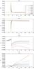	Fig. 3 Same as Fig. 2 for the l = 3 mode.
In the text

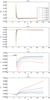	Fig. 4 Same as Fig. 2 for the l = 4 mode.
In the text

	Fig. 5 Contours of the log  nH in units of mH cm-3 along the yz plane. From top to bottom: l = 0, l = 1, l = 2 and l = 3 modes for virial parameter α = 0.006. The units along each axis are parsecs and tff stands for free-fall time.
In the text

	Fig. 6 Contours of the log nH in units of mH cm-3 along the yz plane. From top to bottom: l = 2 mode for virial parameters α = 0.1, α = 0.2 and α = 0.8. Like in Fig. 5, units along each axis are parsecs and tff stands for free-fall time.
In the text

	Fig. 7 Growth rates for α = 0.006 mode for azimuthal wave numbers l.
In the text

	Fig. 8 Growth rates of the l = 0 mode for various virial parameters α.
In the text

	Fig. 9 Growth rates of the l = 2 mode for various virial parameters α.
In the text

References

- Andre, P., Ward-Thompson, D., & Barsony, M. 1993, ApJ, 406, 122 [NASA ADS] [CrossRef] [Google Scholar]
- Andre, P., Ward-Thompson, D., & Barsony, M. 2000, in Protostars and Planets IV (Tucson: University of Arizona Press), 59 [Google Scholar]
- Banerjee, R., & Pudritz, R. E. 2006, ApJ, 641, 949 [NASA ADS] [CrossRef] [Google Scholar]
- Bate, M. R. 2009, MNRAS, 397, 232 [NASA ADS] [CrossRef] [Google Scholar]
- Bonnor, W. B. 1956, MNRAS, 116, 351 [CrossRef] [Google Scholar]
- Boss, A. P., & Bodenheimer, P. 1979, ApJ, 234, 289 [NASA ADS] [CrossRef] [Google Scholar]
- Boss, A. P., & Keiser, S. A. 2013, ApJ, 764, 136 [NASA ADS] [CrossRef] [Google Scholar]
- Burkert, A., & Bodenheimer, P. 1993, MNRAS, 264, 798 [NASA ADS] [CrossRef] [Google Scholar]
- Cha, S.-H., & Whitworth, A. P. 2003, MNRAS, 340, 91 [NASA ADS] [CrossRef] [Google Scholar]
- Chen, X., Launhardt, R., Bourke, T. L., Henning, T., & Barnes, P. J. 2008, ApJ, 683, 862 [NASA ADS] [CrossRef] [Google Scholar]
- Commerçon, B., Hennebelle, P., Audit, E., Chabrier, G., & Teyssier, R. 2008, A&A, 482, 371 [NASA ADS] [CrossRef] [EDP Sciences] [Google Scholar]
- Duchêne, G., Bouvier, J., Bontemps, S., André, P., & Motte, F. 2004, A&A, 427, 651 [NASA ADS] [CrossRef] [EDP Sciences] [Google Scholar]
- Duchêne, G., Bontemps, S., Bouvier, J., et al. 2007, A&A, 476, 229 [NASA ADS] [CrossRef] [EDP Sciences] [Google Scholar]
- Duquennoy, A., & Mayor, M. 1991, A&A, 248, 485 [NASA ADS] [Google Scholar]
- Ebert, R. 1955, ZAp, 37, 217 [Google Scholar]
- Falgarone, E., & Phillips, T. G. 1990, ApJ, 359, 344 [NASA ADS] [CrossRef] [PubMed] [Google Scholar]
- Ghez, A. M., Neugebauer, G., & Matthews, K. 1993, AJ, 106, 2005 [NASA ADS] [CrossRef] [Google Scholar]
- Girart, J. M., Rao, R., & Estalella, R. 2009, ApJ, 694, 56 [NASA ADS] [CrossRef] [Google Scholar]
- Girichidis, P., Federrath, C., Banerjee, R., & Klessen, R. S. 2011, MNRAS, 413, 2741 [NASA ADS] [CrossRef] [Google Scholar]
- Goodman, A. A., Benson, P. J., Fuller, G. A., & Myers, P. C. 1993, ApJ, 406, 528 [NASA ADS] [CrossRef] [Google Scholar]
- Goodwin, S. P., Kroupa, P., Goodman, A., & Burkert, A. 2007, in Protostars and Planets V (Tucson: University of Arizona Press), 133 [Google Scholar]
- Hachisu, I., & Eriguchi, Y. 1984, A&A, 140, 259 [NASA ADS] [Google Scholar]
- Hanawa, T., & Matsumoto, T. 1999, ApJ, 521, 703 [NASA ADS] [CrossRef] [Google Scholar]
- Hennebelle, P., & Teyssier, R. 2008, A&A, 477, 25 [NASA ADS] [CrossRef] [EDP Sciences] [Google Scholar]
- Hennebelle, P., Whitworth, A. P., Cha, S.-H., & Goodwin, S. P. 2004, MNRAS, 348, 687 [NASA ADS] [CrossRef] [Google Scholar]
- Hunter, C. 1964, ApJ, 139, 570 [NASA ADS] [CrossRef] [Google Scholar]
- Jog, C. J. 2013, MNRAS, 434, L56 [NASA ADS] [CrossRef] [Google Scholar]
- Joos, M., Hennebelle, P., Ciardi, A., & Fromang, S. 2013, A&A, 554, A17 [NASA ADS] [CrossRef] [EDP Sciences] [Google Scholar]
- Jørgensen, J. K., Bourke, T. L., Myers, P. C., et al. 2007, ApJ, 659, 479 [NASA ADS] [CrossRef] [Google Scholar]
- Klessen, R. S., & Burkert, A. 2001, ApJ, 549, 386 [NASA ADS] [CrossRef] [Google Scholar]
- Klessen, R. S., Burkert, A., & Bate, M. R. 1998, ApJ, 501, L205 [NASA ADS] [CrossRef] [Google Scholar]
- Larson, R. B. 1969, MNRAS, 145, 271 [NASA ADS] [CrossRef] [Google Scholar]
- Larson, R. B. 1981, MNRAS, 194, 809 [NASA ADS] [CrossRef] [Google Scholar]
- Machida, M. N., Omukai, K., Matsumoto, T., & Inutsuka, S.-I. 2008, ApJ, 677, 813 [NASA ADS] [CrossRef] [Google Scholar]
- Matsumoto, T., & Hanawa, T. 2003, ApJ, 595, 913 [NASA ADS] [CrossRef] [Google Scholar]
- Maury, A. J., André, P., Hennebelle, P., et al. 2010, A&A, 512, A40 [NASA ADS] [CrossRef] [EDP Sciences] [Google Scholar]
- Miyama, S. M., Hayashi, C., & Narita, S. 1984, ApJ, 279, 621 [NASA ADS] [CrossRef] [Google Scholar]
- Myhill, E. A., & Kaula, W. M. 1992, ApJ, 386, 578 [NASA ADS] [CrossRef] [Google Scholar]
- Offner, S. S. R., Klein, R. I., & McKee, C. F. 2008, ApJ, 686, 1174 [NASA ADS] [CrossRef] [Google Scholar]
- Ori, A., & Piran, T. 1988, MNRAS, 234, 821 [NASA ADS] [CrossRef] [Google Scholar]
- Patience, J., White, R. J., Ghez, A. M., et al. 2002, ApJ, 581, 654 [NASA ADS] [CrossRef] [Google Scholar]
- Penston, M. V. 1969, MNRAS, 144, 425 [NASA ADS] [CrossRef] [Google Scholar]
- Price, D. J., & Bate, M. R. 2007, MNRAS, 377, 77 [NASA ADS] [CrossRef] [Google Scholar]
- Shu, F. H. 1977, ApJ, 214, 488 [NASA ADS] [CrossRef] [Google Scholar]
- Teyssier, R. 2002, A&A, 385, 337 [NASA ADS] [CrossRef] [EDP Sciences] [Google Scholar]
- Tohline, J. E. 1981, ApJ, 248, 717 [NASA ADS] [CrossRef] [Google Scholar]
- Tohline, J. E. 2002, ARA&A, 40, 349 [NASA ADS] [CrossRef] [Google Scholar]
- Truelove, J. K., Klein, R. I., McKee, C. F., et al. 1997, ApJ, 489, L179 [NASA ADS] [CrossRef] [Google Scholar]
- Tsuribe, T., & Inutsuka, S.-I. 1999, ApJ, 526, 307 [NASA ADS] [CrossRef] [Google Scholar]
- Whitworth, A., & Summers, D. 1985, MNRAS, 214, 1 [NASA ADS] [CrossRef] [Google Scholar]