| Issue |
A&A
Volume 574, February 2015
|
|
|---|---|---|
| Article Number | A78 | |
| Number of page(s) | 14 | |
| Section | Numerical methods and codes | |
| DOI | https://doi.org/10.1051/0004-6361/201424570 | |
| Published online | 28 January 2015 | |
Photometric brown-dwarf classification
I. A method to identify and accurately classify large samples of brown dwarfs without spectroscopy
1 Astrophysics Group, Imperial College London, Blackett Laboratory, Prince Consort Road, London SW7 2AZ, UK
e-mail: This email address is being protected from spambots. You need JavaScript enabled to view it.
2 Department of Terrestrial Magnetism, Carnegie Institution of Washington, Washington, DC 20015, USA
3 Department of Mathematics, Imperial College London, London SW7 2AZ, UK
4 Department of Physics, University of California, San Diego, CA 92093, USA
5 Institute of Astronomy, Madingley Road, Cambridge CB3 0HA, UK
Received: 9 July 2014
Accepted: 27 November 2014
Abstract
Aims. We present a method, named photo-type, to identify and accurately classify L and T dwarfs onto the standard spectral classification system using photometry alone. This enables the creation of large and deep homogeneous samples of these objects efficiently, without the need for spectroscopy.
Methods. We created a catalogue of point sources with photometry in 8 bands, ranging from 0.75 to 4.6 μm, selected from an area of 3344 deg2, by combining SDSS, UKIDSS LAS, and WISE data. Sources with 13.0 <J< 17.5, and Y − J> 0.8, were then classified by comparison against template colours of quasars, stars, and brown dwarfs. The L and T templates, spectral types L0 to T8, were created by identifying previously known sources with spectroscopic classifications, and fitting polynomial relations between colour and spectral type.
Results. Of the 192 known L and T dwarfs with reliable photometry in the surveyed area and magnitude range, 189 are recovered by our selection and classification method. We have quantified the accuracy of the classification method both externally, with spectroscopy, and internally, by creating synthetic catalogues and accounting for the uncertainties. We find that, brighter than J = 17.5, photo-type classifications are accurate to one spectral sub-type, and are therefore competitive with spectroscopic classifications. The resultant catalogue of 1157 L and T dwarfs will be presented in a companion paper.
Key words: stars: low-mass / techniques: photometric / methods: data analysis / stars: individual: SDSS J1030+0213 / stars: individual: 2MASS J1542-0045 / stars: individual: ULAS J2304+1301
© ESO, 2015
1. Introduction
The first brown dwarfs were discovered by Nakajima et al. (1995) and Rebolo et al. (1995), having been theorised earlier by Kumar (1963a,b) and Hayashi & Nakano (1963). Exploration of the brown dwarf population has proceeded rapidly over the subsequent two decades, enabled by new surveys in the optical, the near-infrared, and the mid-infrared. This has resulted in the creation of three new, successively cooler, spectral classes beyond M: the L (Kirkpatrick et al. 1999; Martín et al. 1999); T (Geballe et al. 2002; Burgasser et al. 2002a, 2006b); and Y dwarfs (Cushing et al. 2011). The temperature sequence has now been mapped all the way down to effective temperatures of ~250 K (Luhman 2014). This almost closes the gap to the effective temperature of gas giants in our Solar System (~ 100 K). The current paper focuses on L and T dwarfs.
One of the fundamental observables that characterises the LTY population is the luminosity function (e.g. Cruz et al. 2007; Reylé et al. 2010) i.e. the dependence of space density on absolute magnitude (or, equivalently, spectral type). The luminosity function can be used to learn about the sub-stellar initial mass function and birth rate. The study of the luminosity function requires a homogeneous sample with well-defined selection criteria.
DwarfArchives.org provides a compilation of L and T dwarfs published in the literature. This collection is heterogeneous, having been culled from several surveys with different characteristics, including, in particular, the Sloan Digital Sky Survey (SDSS; York et al. 2000) in the optical, the Deep Near-Infrared Southern Sky Survey (DENIS; Epchtein et al. 1997), the Two Micron All-Sky Survey (2MASS; Skrutskie et al. 2006) and the UKIRT Infrared Deep Sky Survey (UKIDSS; Lawrence et al. 2007) in the near-infrared, and WISE in the mid-infrared. DwarfArchives.org now contains over 1000 L and T dwarfs but the constituent samples are themselves heterogeneous and so not well suited for statistical analysis.
A good example of the state of the art in obtaining a statistical sample of brown dwarfs is the study of the sub-stellar birth rate by Day-Jones et al. (2013). They classified 63 new L and T dwarfs brighter than J = 18.1, using X-shooter spectroscopy on the Very Large Telescope (VLT), after selecting them through colour cuts. The sample targeted a limited section of the L and T sequence and required substantial follow-up resources: at J ≃ 17.5 a near-infrared spectrum good enough for classification to one spectral sub-type requires about 30 min on an 8 m class telescope.
In this paper we consider how to define a homogeneous, complete sample of field L and T dwarfs, with accurate classifications, over the full L and T spectral range, from L0 to T8, that reaches similar depth and that is more than an order of magnitude larger. Such a sample is useful to reduce the uncertainty in the measurement of the luminosity function and also allows a variety of studies, such as measuring the brown-dwarf scale height (Ryan et al. 2005; Jurić et al. 2008), the frequency of binarity (Burgasser et al. 2006c; Burgasser 2007; Luhman 2012) and, if proper motions can be measured, kinematic studies (Faherty et al. 2009, 2012; Schmidt et al. 2010; Smith et al. 2014). A large sample can also be used to identify rare, unusual objects (e.g. Burgasser et al. 2003; Folkes et al. 2007; Looper et al. 2008).
All previous searches for L and T dwarfs have required spectroscopy for accurate classification. This paper describes an alternative search and classification method that uses only existing photometric survey data. We call the method photo-type, by analogy with photo-z, the measurement of galaxy redshifts from photometric data alone. Section 2 sets out the details of the technique. The method of classification, explained in Sect. 2.1, requires comparison of the multiband photometry of the object against a set of template colours, to find the best fit. The creation of the template set is explained in Sect. 2.2. In Sect. 2.3 we discuss possible sources of bias in the template colours. In Sect. 2.4 we additionally consider the possibility of identifying unresolved binaries by their unusual colours. We then apply the new technique in Sect. 3. In Sect. 3.1 we describe the creation of a catalogue of multi wavelength photometry of point sources with matched photometry in SDSS, UKIDSS, and WISE. The results of a search of this catalogue for L and T dwrafs are provided in Paper II. In Sect. 3.2 we quantify the accuracy of the classification method. Section 4 provides a “cookbook” for photo-type, explaining how to measure the spectral type, and its accuracy, for a source with photometry in all or a subset of the 8 bands used here. We summarise in Sect. 5. In Paper II we present the catalogue of 1157 L and T dwarfs classified by photo-type, and quantify the completeness of the sample.
The photometric bands used in this study are the i and z bands in SDSS, the Y, J, H, K bands in UKIDSS, and the W1, W2 bands in WISE. All the magnitudes and colours quoted in this paper are Vega based. The YJHKW1W2 survey data are calibrated to Vega, while SDSS is calibrated on the AB system. We have applied the offsets tabulated in Hewett et al. (2006) to convert the SDSS iz AB magnitudes to Vega.
2. The technique
2.1. Classification by χ2
The overall aim here is to develop a method to classify every point-source in a multiband photometric catalogue as a star, white dwarf, brown dwarf or quasar, based only on its observed photometry. This could be achieved most rigorously by using Bayesian model comparison (Mortlock et al. 2012). A formalism for doing so is detailed in the Appendix, which also includes the series of approximations and assumptions which lead from the full Bayesian result to the much simpler χ2-based classification we actually use. While some of the approximations below are clearly unrealistic, that is unimportant per se – all that matters in this context is whether the final classifications remain (largely) unchanged. The effect of our approximations are examined in detail at the end of Sect. 2.2, but justified more qualitatively here.
The first approximation is that we work with magnitudes and assume the photometric errors are Gaussian. This is justified at high signal-to-noise ratios (S/N). At low S/N, the correct approach is to work with fluxes (e.g., Mortlock et al. 2012) where, except in the low-photon regime (e.g., X-ray astronomy), the errors are Gaussian. A few T dwarfs in our sample have low S/N in the SDSS i and z bands; for these we use |asinh| magnitudes and errors (Lupton et al. 1999) as the resultant χ2 value is close to that which would have been calculated from the fluxes.
The second simplification is to adopt equal prior probabilities for each of the different (sub-)types. In the limited region of colour–magnitude space that we search for L and T dwarfs, 13.0 <J< 17.5, Y − J> 0.8, the main contaminating population is reddened quasars (see Hewett et al. 2006). At these bright magnitudes this population is easily distinguished, i.e. the priors are not very important. Similarly, provided the priors vary relatively slowly along the MLT spectral sequence and the likelihoods are sharply peaked, the prior probabilities for all the sub-types can be assumed to be equal without affecting the final classifications.
A third, related, approximation is to adopt broad, uniform priors for the magnitude distributions (i.e., number counts) of each type. This again is obviously unrealistic, as the number of L and T dwarfs per magnitude is expected to be N(m) ∝ 103m/ 5, as they are an approximately uniform population in locally Euclidean space. But the form of this prior has minimal impact on the classifications because we are operating in the high S/N regime in which the data constrain the overall flux-level of a source to a narrow range.
Applying the above assumptions and approximations to the full Bayesian formalism, described in the Appendix, results in the following classification scheme:
-
1.
The first requirement is photometric data on the source to beclassified: the measuredmagnitudes,
 , and uncertainties, { σb }, in each of Nb bands (with b ∈ { 1,2,...,Nb })1. For most sources considered here Nb = 8 and the filters are izYJHKW1W2.
 -
2.
The other required input is a set of Nt source types, each specified by a set of template colours, { cb,t }, which give the magnitude difference between band b and some reference band B for objects of type t (with t ∈ { 1,2,...,Nt }). Hence cB,t = 0 by construction, meaning that the magnitude in this reference band, mB, is the natural quantity to specify the overall source brightness. Here we use J as the reference band as our conservative magnitude cuts in this band ensure that mB = mJ is well constrained.
-
3.
The first processing step is, for each of the Nt types, to calculate the inverse variance weighted estimate of the reference magnitude,
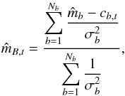 (1)which, in general, is different for each template.
 -
4.
Next, the above value for
 is used to calculate the minimum χ2 value for type t,
 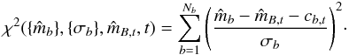 (2)It is important that χ2 is calculated by comparing measured and predicted magnitudes, as opposed to colours. The reasons for this are given in the Appendix.
 -
5.
Finally, the source is classified as being of the type t which results in the smallest value of
 . The conditions under which this corresponds to the most probable type are detailed in the Appendix; a more empirical demonstration that this results in a reliable classification is given in Sect. 4.
2.2. Templates
The templates used in photo-type fit quasars, white dwarfs, stars and brown dwarfs. The template colours for quasars were taken from Maddox et al. (2012). Templates for quasars with weak, typical, and strong lines were included, for a range of reddening, E(B − V) = 0.00,0.10,0.20,0.30,0.40,0.50, for the redshift range 0 <z< 3.4. The template colours for white dwarfs and main-sequence stars earlier than M5 used in this work are taken from Hewett et al. (2006). These are included for completeness, but in fact are not relevant for objects with colour Y − J> 0.8. The star and quasar templates only cover the bands izYJHK and were used in the initial selection of candidate L and T dwarfs, before the classifications were refined by including the WISE colours, as explained in Sect. 3.
The templates in Hewett et al. (2006) for stars of class M5 and later, and for L and T dwarfs, were found to be inadequate for accurate classification. These colours were computed from spectra, and before any Y band data with UKIDSS had been taken. Now that UKIDSS is complete it is possible to improve on the colour relations of ultra-cool dwarfs using photometry of known sources within the UKIDSS footprint. These will be more accurate than colours computed from spectra, in particular for the z band where the computed fluxes are very sensitive to the exact form of the red cutoff of the band, defined by the declining quantum efficiency of the CCDs.
To compute template colours for ultracool dwarfs we fit polynomials to colours of known dwarfs as a function of spectral type, as shown in Figs. 1 and 2. We searched DwarfArchives.org, and additional recent published samples (Sect. 2.3), for spectroscopically classified L and T dwarfs within the UKIDSS DR10 footprint. In Sect. 3.1 we describe the creation of a catalogue of point sources matched over 3344 deg2 of SDSS, UKIDSS DR10, and WISE, in the magnitude range 13.0 <J< 17.5, with Y − J> 0.8. Of the sample of spectroscopically classified L and T dwarfs, 190 appear in our catalogue i.e. are classified as stellar, have reliable matched photometry in izYJHKW1W2, and meet the magnitude and colour selection criteria2. Our fundamental assumption is that the measured colours of these sources are representative of the colours of the L and T populations. Within this sample there are 150 L dwarfs and 40 T dwarfs. We discuss possible bias of this sample in the next section. We supplemented the sample of L and T dwarfs with 111 cool M stars of spectral type M5 to M9 from the SDSS spectroscopic catalogue (Ahn et al. 2012) in order to tightly constrain the polynomials at the M/L boundary.
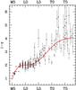 |
Fig. 1 i − z colour vs. spectral sub-type for MLT dwarfs in the UKIDSS LAS DR10 footprint. The error bars plotted show the random photometric errors. The fitted curve provides the template colours listed in Table 1. In making the fit, a colour error of 0.07 mag. (i.e. 0.05 mag. in each band) is added in quadrature to the random photometric errors to account for intrinsic scatter in the colours. The very large errors in the T dwarf regime mean that the curve is poorly defined in this region, as discussed in the text. The vertical scale is the same as in Fig. 2. The outlying blue T0 dwarf is discussed in Sect. 3.2. All photometry is on the Vega system. |
The 40 T dwarfs are classified on the revised system of Burgasser et al. (2006b), based on near-infrared spectroscopy, and so our colour fits are anchored to this system for T dwarfs. Of the 150 L dwarfs, 116 have optical classifications on the system of Kirkpatrick et al. (1999), and of these 16 also have near-IR classifications. For these 16 cases we averaged the two classifications quantised to the nearest half spectral sub-type. The remaining L dwarfs have near-IR classifications only. Of the near-IR classifications, close to half use the SpeX prism spectral library (Burgasser 2014)3, which is anchored to Kirkpatrick et al. (1999), while the remainder use the index system of Geballe et al. (2002). Since we wish photo-type to be anchored to the optical classification system we checked for any bias introduced by including the near-IR spectral types. We computed template colours, as described below, for the two cases, including and excluding near-IR spectral types for the L dwarfs. We then classified a large sample of L dwarfs (the 1077 described in Sect. 3) using both sets of templates and looked at the differences in spectral type for the two sets of templates. The result was a negligible offset, μ = 0.06 spectral types, and small scatter, σ = 0.23, with no clear trends with spectral type, confirming that for L dwarfs photo-type is accurately anchored to the optical system of Kirkpatrick et al. (1999).
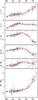 |
Fig. 2 Colours z − Y, Y − J, J − H, H − K, K − W1, W1 − W2 vs. spectral sub-type for MLT dwarfs in the UKIDSS LAS DR10 footprint. The errorbars plotted show the random photometric errors. The fitted curve provides the template colours listed in Table 1. In making the fit, a colour error of 0.07 mag. (i.e. 0.05 mag. in each band) is added in quadrature to the random photometric errors to account for intrinsic scatter in the colours. The vertical scale is the same as in Fig. 1. All photometry is on the Vega system. |
Although the SpeX prism near-infrared spectral library for L dwarfs is tied to the optical classification scheme of Kirkpatrick et al. (1999), there exist spectrally peculiar sources where the optical and near-IR classifications differ, in some cases by more than two spectral sub-types. In the same way, for peculiar sources the photo-type classifications may differ from the optical classifications. One of the virtues of the photo-type method is that it provides both a best-fit spectral type, and a goodness of fit statistic (the multi-band χ2) which can be used to identify peculiar sources. In this sense it provides more information than a simple classification based on optical spectroscopy or near-infrared spectroscopy alone.
Denoting colour by c and spectral type by t, with numerical values M5−M9 as 5−9, L0−L9 as 10−19 and T0−T8 as 20−28, we fit polynomials  via χ2 minimisation4, over the 8 bands.
In the development of this analysis it was immediately clear that the scatter in the colours is larger than the typical photometric error i.e. there is an intrinsic scatter in the colours, due e.g. to variations in metallicity, surface gravity, cloud cover, and unresolved binaries in the sample, as well as uncertainty in the spectral classification. It is important to allow for this scatter in fitting the curves, or the fits could be affected by outlying points with small photometric errors.
We estimated the intrinsic scatter for each colour in an iterative fashion as follows. We first guessed the intrinsic scatter by eye, and added this value in quadrature to the photometric error on each point. We then found the lowest order polynomial that provided a good fit to the data. We then re-estimated the intrinsic scatter as the value that, added in quadrature to the photometric error on each point, and summed over all points, matched the measured variance about the fitted polynomial, having identified and removed any discrepant outliers. Averaging over all the colours we measured an intrinsic scatter of 0.07 mag, which we adopted as the intrinsic scatter for all colours. The implementation involved adding 0.05 mag. error (i.e.  ) in quadrature to the photometric error in each band for every object. This may be viewed as the uncertainty on the templates.
Having established a suitable value for the intrinsic scatter in the colours, the polynomials were refit, starting with a linear fit, and then successively increasing the order of the polynomial, only provided a significant improvement in the fit was achieved, Δχ2> 7, in order to prevent over-fitting5. In most cases a fourth or fifth order polynomial was sufficient. The fitted polynomials are shown in Figs. 1 and 2. The coefficients of the polynomials are provided in Table 2, and the template colours are provided in Table 1.
An additional source of error that should be accounted for in classifying sources is the uncertainty in the polynomial fits themselves. Since some curves are more tightly constrained by the data than others, by incorporating this uncertainty, and its variation with spectral type, the different curves are then correctly weighted. We have established the uncertainties from the covariance matrices of the polynomial fits, and the results are plotted in Fig. 4. We have incorporated these errors in classifying sources, and found that in fact they have no significant influence on the classifications. The analysis leading to this conclusion is presented in Sect. 3.2.3.
Template colours of M5–T8 dwarfs.
A number of the individual colour plots are discussed below:
-
i − zcolour: the i − z colour polynomial is not well defined for T dwarfs. This is because nearly all the T dwarfs are very faint in the i band, and so the errors are large, ~ 0.5 mag. or greater. It would be useful to measure accurate i − z colours for this sample in order to better establish the shape of the curve and the intrinsic scatter, but this is difficult because the z band used will have to match the SDSS passband very closely (as explained above). In practise the difficulty of measuring the i − z curve accurately in the T dwarf regime is not critical because, of course, most of the candidates are very faint in i, and so have large photometric errors, meaning that the contribution to the total χ2 from the i band is relatively small. We show later (Sect. 3.2.3) that including the i band improves the accuracy of the classification of L dwarfs, but not of T dwarfs.
-
Y − Jcolour: we found we were unable to fit the Y − J curve satisfactorily with a single polynomial. We attribute this to a discontinuity in the relation near spectral type L7. From inspection of the SpeX spectra of the near-IR spectral standards the jump appears to be associated with the rapid weakening of FeH absorption in the Y band between spectral types L6 and L8 (Burgasser et al. 2002b). To check, and to decide where to impose the discontinuity, we computed synthetic colours from the SpeX near-IR spectral standards. These are provided in Table 3 (Sect. 3.2), and show a break in Y − J colour between L7 and L8. We therefore fit two separate polynomials to the data, with a quadratic for types ≤L7, and a linear fit for types ≥L8, joined by a straight line from L7 to L8. The step between L7 and L8 is 0.14 mag. In Paper II we show the same Y − J plot for the new sample of L and T dwarfs, and the jump is seen more clearly in the larger sample.
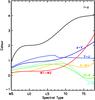
Fig. 3 Colour curves from Figs. 1 and 2 plotted in a single figure in order to compare the relative usefulness of different colours in classifying different spectral types in the LT sequence.
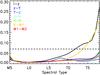
Fig. 4 Uncertainties of the fits of the colour polynomials as a function of spectral type. With the exception of the i − z and K − W1 curves the uncertainties are significantly smaller than the intrinsic scatter (marked by the dashed line).
-
J − H, J − Kcolours: the flattening and return of the colour to redder values at the end of the T sequence appears to be real, rather than an artefact of the fitting procedure, as it can also be seen in the plots in Leggett et al. (2010) and Cushing et al. (2011).
Figure 3 illustrates the usefulness of different colours in the classification of dwarfs of different spectral type. The steeper the curve, the more accurate the classification, with the exception of i − z in the T dwarf region where the errors are larger. Therefore it is evident that spectral classification will be most accurate in the region from about T1 to T5, because in this region several of the colour relations are steep, whereas around L6 several of the colour curves are rather flat and classification will be less accurate. We quantify the accuracy of classification in Sect. 3.2.
Colour polynomials of M5–T8 dwarfs.
2.2.1. Priors for classification
We now return to the assumption of flat priors for all the templates. To check the potential contamination of the sample by quasars, we used the quasar templates as synthetic sources (adding photometric errors as appropriate) and picked out the quasar, from the full set, that provided the best-fit to any dwarf along the sequence L0 to T8. The best match between the two template sets is a reddened quasar E(B − V) = 0.5 of redshift z = 2.7 matched to a L1.5 dwarf, for which the goodness of fit is χ2 = 92 (for six degrees of freedom). With such a poor fit it is clear that L and T dwarfs will be easily discriminated from reddened quasars, independent of priors, within reason.
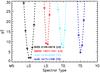 |
Fig. 5 χ2 (computed from Eq. (2)) against spectral type, in the classification of four known L and T dwarfs, as follows: SDSS J0149+0016 (L0, J = 17.18±0.03), 2MASS J1407+1241 (L5, J = 15.33±0.004), ULAS J1516+0259 (T0, J = 16.88±0.02), and ULAS J1417+1330 (T5, J = 16.77±0.01). In each case the χ2 curves show no degeneracies, and are sharp, indicating accurate classification (quantified in Sect. 3.2). |
In a flux-limited sample early L dwarfs are much more common than late L dwarfs. Because of uncertainty in the classifications, the assumption of flat priors along the LT sequence will lead to a bias in the classifications (akin to Eddington bias). The extent of the bias depends on the luminosity function and on the precision of the classifications i.e. how sharp the curve of χ2 against spectral type is. In Fig. 5 we plot χ2 against spectral type for four known L and T dwarfs from the sample of 190 previously known dwarfs. These plots show that the χ2 minimum is very sharp and unambiguous, minimising any bias in the classification. The Eddington bias will be corrected for in computing the luminosity function in a future paper.
2.3. Possible sources of bias in the colour relations
In this section we discuss possible bias in the derived colour relations. This issue is closely related to the question of completeness, but we defer a detailed discussion of the completeness of the new sample to Paper II. As stated in Sect. 2.2, our fundamental assumption is that the sample of 190 L and T dwarfs used to define the polynomial colour relations is representative of the L and T population i.e. the mean and spread in colour at each spectral type. We first examine reasons for missing a few of the catalogued objects.
We searched DwarfArchives (update of 6th of November 2012) for known L and T dwarfs with 13.0 <J< 17.5 in the UKIDSS LAS YJHK footprint, supplemented by the recent samples of Burningham et al. (2013), Day-Jones et al. (2013), Kirkpatrick et al. (2011), and Mace et al. (2013). A few sources with unreliable photometry in any of the eight bands (e.g. blended with a diffraction spike, or landing on a bad CCD row) were discarded. In addition, three sources were classified as stellar in 2MASS, but appear elongated in UKIDSS because they are binaries. This means there is a small bias against finding binaries where the angular separation of the pair is a few tenths of an arcsec, but this should not have any significant effect on the colour relations. The final sample comprises 192 known L and T dwarfs in the surveyed area, with reliable photometry, and classified as stellar.
A further two sources are missing from our sample:
-
WISEPC J092906.77+040957.9: this is a T6.5 dwarf discoveredby Kirkpatrick et al. (2011). Thesource was missed because its motion between the epochs of theY and K UKIDSS observations was
 , which is just greater than the
  UKIDSS internal matching criterion.
 -
SDSS J074656.83+251019.0: this source is an L0 dwarf discovered by Schmidt et al. (2010). It has Y = 17.37, and J = 16.58, giving Y − J = 0.79, meaning it is just bluer than our selection limit Y − J = 0.8. A second epoch J measurement gave J = 16.60. The source is apparently anomalously blue in Y − J, as the typical colour of an L0 dwarf is Y − J = 1.04 (Table 1).
The inclusion of these two sources would not significantly affect the colour relations. Therefore whether the colour polynomials are biased is a question of whether the sample in DwarfArchives contains significant colour selection biases, or whether there are any significant populations of L and T dwarfs with peculiar colours that remain undiscovered.
The samples of Kirkpatrick et al. (2011) and Mace et al. (2013), contain many late T dwarfs selected with WISE. To check specifically the W1 − W2 relation we created a comparison sample after excluding those sources already used in the curve fitting (i.e. those in the UKIDSS LAS footprint). We compared the W1 − W2 polynomial obtained for this catalogue to our template polynomial, finding it to be identical to within 0.01 mag. over the full LT range.
We also re-examined the bias, noted by Schmidt et al. (2010), that early L dwarfs in DwarfArchives (at the time) were on average redder in J − K by ~ 0.1 mag than those in their much larger sample. Schmidt et al. (2010) selected sources for spectroscopy with a sufficiently blue cut in i − z to ensure they included all L dwarfs, and so their J − K colours should be unbiased. This large sample is now included in DwarfArchives, so any bias is much reduced. Schmidt et al. (2010) ascribed the bias in the older DwarfArchives sample to the colour cut J − K> 1.0 applied by Cruz et al. (2003) in selecting L dwarfs, meaning that bluer L dwarfs were excluded. The extent of the bias introduced by a colour cut would depend on both the intrinsic spread in J − K colour, as well as the random errors. Our own analysis, which uses the much more precise UKIDSS photometry rather than the original 2MASS photometry, finds a smaller bias between these two samples of 0.05 mag over the spectral type range L0 to L4. Our analysis suggests that much of the original bias noted was due to random photometric errors, rather than true colour bias. Accounting for the relative sizes of the two samples used in the analysis, any remaining bias in our J − K colour relation would be ≲ 0.01 mag.
It remains to consider the possibility that significant populations with substantially different colour relations are underrepresented in DwarfArchives. These might include unusually blue objects, such as SDSS J074656.83+251019.0 (discussed above), or unusually red objects (Faherty et al. 2013; Liu et al. 2013). Such a population would have a significant influence, e.g. a shift in the colour relations of > 0.03 mag., if, for example, the population comprised, say, 10% of the entire L and T population, and their colours were unusual by 0.3 mag. There is no indication in the polynomial plots (Figs. 1 and 2) of any outlying clouds of points that might hint at such a population. But given the large differences between the L and T population and quasars (Sect. 2.2), photo-type should pick up unusual L and T dwarfs, which will be identifiable in the new sample. We reconsider this question in Paper II.
2.4. Unresolved binaries
A small number of sources are classified as L or T but with large χ2. These objects may be peculiar single sources, or could be unresolved binaries. To check whether any might be unresolved binaries, we created template colours for all possible L+T binary combinations, over the range of spectral types L0 to T8. We use the relation between absolute magnitude in the J band and spectral type from Dupuy & Liu (2012) to provide the relative scaling of the two templates, hereafter referred to as S1 and S2. Then for sources with large χ2, we compare the improvement in χ2 achieved by introducing the extra degree of freedom of a binary fit. Objects with Δχ2> 7 (where 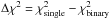 ) are accepted as candidate binaries.
The search for candidate unresolved binaries is effective only over particular regions of the S1, S2 parameter space because, given the colour uncertainties, some binary combinations S1+S2 are satisfactorily fit by the colours of a single source. For example, the colour template for the combination L0+T5 is very similar to the colour template of a L0 dwarf. This issue is illustrated in Fig. 6. Here we tested the improvement of a binary fit over a single fit for different combinations S1+S2. Each point in the grid represents a binary S1+S2. We created synthetic template colours for the binary, adding random and systematic errors as before. Then for each artificial binary we found the best fit single solution and the best fit binary solution, and recorded the improvement in χ2. The contours plot the average improvement in χ2 achieved with the binary fit, and therefore map out regions where photo-type is sensitive to the detection of binaries.
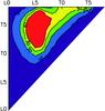 |
Fig. 6 Contour plot illustrating sensitivity to detection of unresolved binaries. The axes correspond to the two components of a binary. The contours plot the improvement in χ2 of a binary dwarf solution over the best single dwarf solution. |
In Paper II we present spectra of some sources identified as candidate binaries using photo-type.
3. Application
In this section we describe the creation of a catalogue of point sources matched across 3344 deg2 of SDSS, UKIDSS and WISE that we search for L and T dwarfs. We also quantify the accuracy of the photo-type method.
3.1. Photometric data
Our study is concerned with field (as opposed to cluster) brown dwarfs and uses survey data at high Galactic latitudes. The starting point for the search is the Data Release 10 (DR10) version of the UKIDSS Large Area Survey (LAS) which provides photometry in the YJHK bands. Point sources are matched to the SDSS and ALLWISE catalogues, to add, respectively, iz and W1W2 photometry. Sources are then classified using the full izYJHKW1W2 data set. The footprint of the survey is defined by the 3344 deg2 area of the UKIDSS LAS, where all four of the YJHK bands have been observed, contained within the SDSS DR9 footprint. All sources also possess WISE photometry from the ALLWISE catalogue.
Creating a matched catalogue requires careful consideration of the image quality, pixel scale, and flux limits of the different surveys. The pixel scales of UKIDSS and SDSS are the same,  , and the two surveys are well matched in terms of image quality: the typical seeing in UKIDSS is
  (Warren et al. 2007), and in SDSS is
  (Adelman-McCarthy et al. 2007). The WISE raw images on the other hand have large pixels,
  , and the full width at half maximum of the W1 and W2 point spread function (PSF) is 6″. The larger PSF results in significant blending of images, leading to incorrect photometry. Such cases are identified by visual inspection of the spectral energy distributions and the images. In the final catalogue, the 7% of sources blended in WISE are classified using only the 6-band izYJHK photometry.
We chose the UKIDSS J band for defining the flux range of the survey, and selected J = 13.0 as the bright limit, to avoid saturation in any band. The faint limit of J = 17.5 was chosen from detailed consideration of the SEDs of L and T dwarfs, and the detection limits in each band, as described below. It corresponds to the maximum depth at which a complete sample with accurate classifications can be defined, given the data. The average 5σ detection limit in J is 19.6, so at J = 17.5 the S/N of sources is about 35. Using the template colours for the L and T sequence (Sect. 2.2), we created synthetic catalogues, with appropriate photometric errors, for different possible J flux limits, and compared the synthetic photometry against the detection limits in each of the other 7 bands. Moving progressively fainter in J, the first objects to fall below any of the detection limits are a small fraction of the coolest T dwarfs, by J = 16.5, absent from SDSS (i.e. fainter than the detection limit in both i and z). Therefore to extend the depth of the survey we implemented a procedure to include sources undetected in SDSS.
The difficulty here is compounded by the fact that T dwarfs, being nearby, can have significant proper motions. Given the epoch differences between the optical and near-infrared observations, typically a few years, this requires a search radius of several arcsec. Then, in some cases, the nearest SDSS match to the UKIDSS target may be the wrong source. The procedure we adopted was to find all SDSS sources within a large search radius of 10″ about the UKIDSS source. Starting with the SDSS match nearest to the target we checked whether there was a different UKIDSS source closer to the SDSS source, and if so eliminated the SDSS source as a match to our target, and proceeded to the next nearest match. Sources that were not matched by this procedure to any source within the 10″ search radius were retained. This allowed us to extend the depth of the survey to J = 17.5. At J = 17.5 some sources fall below the detection limit in other bands. The incompleteness due to this is very small and is quantified below.
In detail, the matching procedure adopted was as follows. From the UKIDSS LAS database we selected objects detected in the full YJHK set, classified as stellar, using -4<mergedclassstat6<4. We also eliminated sources with questionable photometry using the quality flag pperrbits<255 in each band. Sources are matched to SDSS as described above. The izYJHK catalogue, 13.0 <J< 17.5, contains 6 775 168 sources. The procedure to match to WISE is cumbersome, so we reduced the size of the catalogue before matching to WISE, while retaining all the L and T dwarfs, as follows. L and T dwarfs are redder in Y − J than all main-sequence stars. So to find L and T dwarfs we can make the problem more manageable by taking a cut in Y − J. In Sect. 2.2 we show that the bluest L or T dwarf template, for type L0, has colour Y − J = 1.04, and that the intrinsic scatter in colours is ~ 0.07. On this basis we applied a cut at Y − J> 0.8, to produce a sample of 9487 sources. From this sample we then visually checked all sources classified as missing in SDSS, eliminating obvious errors (due e.g. to blending or bad rows). In a small number of cases, where the undetected object is just visible, we undertook aperture photometry of the SDSS images using the Image Reduction and Analysis Facility (IRAF; Tody 1986)7.
The sample at this stage is dominated by late M dwarfs. To reduce the sample size further, before matching to WISE, we made a first-pass classification, using the method described in Sect. 2.1, from the combined izYJHK photometry, and then limited our attention to the 7503 sources classified as cool dwarfs, with classification M6 or later. All these sources were then matched to WISE, using a 10″ search radius, to extract the W1 and W2 photometry. Only one source, classified by photo-type as L1.58, was unmatched to WISE, because it is just below the detection limit. It is retained, together with its UKIDSS+SDSS classification. The final, refined, classifications were obtained from the full izYJHKW1W2 photometry. All candidate L and T dwarfs were visually inspected in all bands. We also plotted up the multiwavelength photometry to identify likely spurious data.
Finally, we quantified any incompleteness in the original UKIDSS YJHK catalogue due to objects falling below the detection limit in any band. Because of their blue J − K colours, at J = 17.5 late T dwarfs have K ~ 18, and a few sources in the tail of the random photometric error distribution might be scattered fainter than the detection limit in K. We undertook a full simulation to quantify the incompleteness, accounting for the UKIDSS detection algorithm, random photometric errors, the intrinsic spread in J − K colour (Sect. 2.2), and the variation in detection limit across the survey. The result is that, integrating over the volume of the survey, the incompleteness is < 0.2% for all spectral types, except T6 and T7 where the incompleteness is 0.6% and 1.2%, respectively.
In summary, from an area of 3344 deg2 we have selected all stellar sources 13.0 <J< 17.5 detected in YJHK in the UKIDSS LAS, and produced a catalogue of 7503 sources with Y − J> 0.8, matched to SDSS and WISE, that are classified as cool dwarfs, M6 or later, from their izYJHK photometry. This is the starting catalogue for a search for L and T dwarfs. A handful of sources are undetected in SDSS or WISE, but these are included in the catalogue. Incompleteness due to sources not detected in any of the YHK bands is negligible.
Classification by photo-type using the full izYJHKW1W2 photometry produced a sample of 1157 L and T dwarfs. This sample is described in Paper II.
Of the 190 sources used in the polynomial fitting, all but one are successfully classified by photo-type as ultra-cool dwarfs. The exception is the unusual L2 dwarf 2MASS J01262109+1428057 discovered by Metchev et al. (2008), which was better fit by a reddened quasar template. Therefore, of the 192 known L and T dwarfs with reliable photometry in the surveyed area and magnitude range, 189 are recovered by our selection and classification method.
3.2. Classification accuracy
In this subsection we estimate the accuracy of photo-type. To recap, for a source measured in izYJHKW1W2, an intrinsic uncertainty of 0.05 mag is added in quadrature to the photometric error in each band, and then the χ2 of the fit to each template is measured, using Eqs. (1) and (2) from Sect. 2.1. The template providing the minimum χ2 fit provides the classification. We estimate the accuracy of the classification in three ways.
-
In the first case we see how accurately we recover thespectroscopic classifications of the 189 sourcesfrom DwarfArchives.
-
Because this sample is heterogeneous, with classifications based on spectra covering different wavelength ranges, we also obtained our own follow-up spectra of candidates from Paper II, to obtain a second assessment of the classification accuracy, from a homogeneous spectroscopic sample.
-
The third estimate uses Monte Carlo methods to create artificial catalogues of colours of all spectral types, over the magnitude range of the catalogue, to estimate the classification accuracy as a function of spectral type and magnitude. We also investigate by how much the accuracy degrades as different bands are removed, to quantify the usefulness of those bands.
There is good agreement between the various methods discussed in Sects. 3.2.1–3.2.3 that classification by photo-type is accurate to a root mean square error (rms) of one spectral sub-type over the magnitude range of the sample.
3.2.1. Comparison against known sources from DwarfArchives
In Fig. 7 we plot the photo-type classification against the spectroscopic classification for the 189 L and T dwarfs from DwarfArchives (i.e. excluding the single misclassified source), together with 111 M stars. The vertical scatter in this plot is a measure of the accuracy of the classification. There is a contribution to the variance from the quantisation of the spectral classification. Therefore for this plot the photo-type classifications were measured to the nearest half sub-type, by interpolating the colours in Table 1. This reduces the contribution of quantisation to the variance, in order to be able to measure the scatter accurately. To account for outliers we estimate the vertical scatter in this plot using the robust estimator 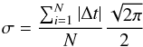 (3)where Δt is the difference between the photo-type classification and the spectroscopic classification. The three outliers marked are discussed below. For the L and T dwarfs we measure, respectively, σL = 1.5 and σT = 1.2. This may be considered an upper limit to the uncertainty in the type because there is a contribution to the scatter from the spectroscopic classification itself. Some of this scatter comes from the fact that spectroscopic classification is based on a restricted portion of the photometric wavelength range covered in this study (0.75 − 4.6 μm). A peculiar source might have a different spectral sub-type if classified in the optical or the near-infrared. The photo-type method will smooth out such differences because of the broad wavelength coverage. This discussion suggests that σ = 1 is a reasonable assessment of the accuracy of photo-type. There is an element of circularity in using the same L and T dwarfs used to define the colour templates in measuring the classification accuracy. In principle this should not be a concern, since the number of objects used is very much greater than the number of parameters in the fitting. Nevertheless it motivates checking the classification accuracy by other means.
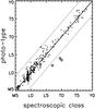 |
Fig. 7 Comparison of photo-type classification vs. spectroscopic classification for the 189 known L and T dwarfs from DwarfArchives, as well as 111 late M stars. Classifications were computed to the nearest half spectral sub-type. Because the classifications are quantised, small offsets have been added in order to show all the points. The dashed lines mark misclassification by four spectral sub-classes. The three outliers marked by diamonds are discussed in the text. |
There are three sources in the plot, marked by diamonds, where the photo-type classifications differ from the spectroscopic classifications by more than four sub-types. These outliers are now discussed in detail.
-
SDSS J1030+0213 was discovered by Knappet al. (2004), and classified asL9.5 ± 1.0 from a near-infrared spectrum. Its type varies somewhat depending on which spectral indices are used: <T0 (H2O in J), T1 (H2O in H), T0.5 (CH4 in H) and L8 (CH4 in K). Using the full 8-band photometry photo-type provides a classification of L4 with χ2 = 20.99, i.e. a relatively poor fit, whereas the L9.5 template has χ2 = 35.43. The two fits are illustrated in Fig. 8. The object has i − Y = 3.32±0.25, which is unusually blue compared to the template colour i − Y = 4.45 for L9.5. Neither model fits the W2 data satisfactorily. Radigan et al. (2014) found that objects around the L/T transition can show significant variability, which provides a possible explanation for the poor fits, since the various photometric data were taken at different dates.
-
2MASS J1542-0045 was discovered by Geißler et al. (2011), who classified it as a peculiarly blue L7, from a near-infrared spectrum. Our best fit is L2, with χ2 = 19.09, while the L7 fit gives χ2 = 319.82. The SED of the source and the two fits are plotted in Fig. 9. Optical spectroscopy of this source would clearly be useful, as noted also by Geißler et al. (2011). The relatively high χ2 of the photo-type best fit would have marked it down as an object worthy of further study.
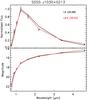
Fig. 8 SED of the source SDSS J1030+0213 compared to the photo-type classification of L4 (black line), and the spectroscopic classification of L9.5 (red line). The upper plot uses flux (fλ), normalised to J, and the lower plot uses magnitudes.
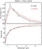
Fig. 9 SED of the source 2MASS J1542-0045 compared to the photo-type classification of L2 (black line), and the spectroscopic classification of L7 (red line). The upper plot uses flux (fλ), normalised to J, and the lower plot uses magnitudes.
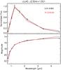
Fig. 10 SED of the source ULAS J2304+1301 compared to the photo-type classification of L3.5 (black line), and the spectroscopic classification of T0 (red line). The upper plot uses flux (fλ), normalised to J, and the lower plot uses magnitudes.
-
ULAS J2304+1301 was discovered by Day-Jones et al. (2013) who classified it T0, from a near-infrared spectrum. The source is classified L3.5 by photo-type with a satisfactory χ2 = 4.82. In contrast, fitting the T0 template yields χ2 = 216.24, a very poor fit. The two fits are compared against the SED of the source in Fig. 10. As can be seen, the source is substantially bluer than a T0 in both i − z and W1 − W2. The source has i − z = 2.18±0.13 (Vega), and is visible as the T0 outlier in Fig. 1. This compares to the expected colour i − z = 2.15 for an L3.5 dwarf, and i − z = 3.36 for a T0 dwarf (Table 1). We have checked the SDSS images which appear normal. It is possible the source is an unresolved binary, and spectroscopy in the iz region would be revealing. Nevertheless given the fact that a single L3.5 provides a satisfactory fit to the photometry, this could be an example of an unresolved binary that cannot be identified from colours alone, as prefigured in Sect. 2.4. It provides a warning that if a spectrum over a limited wavelength range provides a substantially different classification to the photo-type classification, the source may be an unresolved binary.
List of SpeX Prism Spectral Library “standards”.
Details of the eight sources observed with SpeX.
3.2.2. SpeX follow up
A cleaner estimate of the accuracy of photo-type may be obtained from uniform high-quality spectra over a wide wavelength range, using the same instrumental set-up, to ensure uniform accurate spectral classifications. For this purpose we selected a sample of objects from the catalogue of Paper II for follow-up observations. We limited the sample to sources with χ2< 15, for the fits to the 8-band photometry, to avoid outliers (objects with large χ2 are considered in detail in Paper II). Other than that we selected objects at random from a range of spectral types.
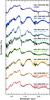 |
Fig. 11 SpeX spectra of eight sources used to estimate the accuracy of photo-type. The sources are classified as L1 (ULAS J0026+0632), L1 (ULAS J0109+0625), L8 (ULAS J0246+0156), L1 (ULAS J0741+2316), L1 (ULAS J0849+2739), T3 (ULAS J0915+0531), L9.5 (ULAS J1029+0620), and M9 (ULAS J1053+0452), by comparison against the spectroscopic standards listed in Table 3. The standard closest in spectral type is also shown for each source. |
We obtained spectra of the 8 sources listed in Table 4 with the SpeX instrument on the NASA Infrared Telescope Facility between March and November 2013. The data were reduced using the SpeXtool package version 3.4 (Cushing et al. 2004). The spectra are plotted in Fig. 11.
The spectra were classified by one of us (JKF), by visual comparison against the SpeX Prism Spectral Library maintained by AJB, and without knowledge of the photo-type classifications. The standards are listed in Table 3. The resulting spectroscopic classifications are listed in Table 4, where they are compared to the photo-type classifications. All objects are confirmed as ultra cool dwarfs. Taking the spectroscopic classification to be the correct classification, the accuracy of photo-type estimated from this small sample is only 0.4 sub-types rms
In all, including peculiar objects (Paper II), so far we have observed 20 objects from our list of L and T dwarfs, and all are ultra-cool dwarfs. This indicates, at least, that the contamination of the L and T sample of Paper II is not large. Nevertheless a larger spectroscopic sample would be required to quantify this accurately.
3.2.3. Simulated data
A third estimate of the accuracy of photo-type was obtained by Monte Carlo methods. For a particular J magnitude and for each spectral type, we created synthetic data, accounting as appropriate for the photometric errors and the intrinsic scatter in the colours of the population (by adding an error of 0.05 mag in each band in quadrature to the photometric error, Sect. 2.2). Then we classified every synthetic object, and measured the dispersion in the classification about the input spectral type. In Fig. 12 we show the measured dispersion for J = 16.0, and at the sample limit J = 17.5. This analysis indicates that the classification method is accurate to better than one spectral type, for all spectral types, even at the sample limit, J = 17.5. The plot shows that the method performs least well, around spectral type L6, as expected (see discussion in Sect. 2.2), because several of the colour relations are relatively flat around this spectral type.
We can use the same apparatus to quantify the usefulness of the different photometric bands, by simply removing one or more bands, and observing the effect on the classification accuracy. We found that the i band contributes usefully to the classification of L dwarfs, but that for our dataset the i band makes a negligible contribution to the classification of T dwarfs, because the photometric errors are so large. The WISE data are useful in classifying all spectral types. The improvement in the classification accuracy depends on spectral type and brightness, but on average including the WISE data reduces the uncertainty in the spectral type by ~ 30%.
Finally we looked at the effect on the classification accuracy of disregarding the uncertainties of the polynomial fits. We found that including or excluding this error term has a negligible effect on the accuracy of the classification for our SDSS/UKIDSS/WISE dataset. For most bands and spectral types this is because the fit error is smaller than the intrinsic colour scatter, as shown in Fig. 4. Even the large fit errors for the i − z and K − W1 colours for late T dwarfs do not influence the classification. The reason for this is that these colours are in any case unimportant in classifying late T dwarfs, where the W1 − W2 colour makes the main contribution.
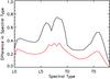 |
Fig. 12 Estimated accuracy rms of the photo-type classification for sources of J = 16.0 (red curve) and J = 17.5 (black curve) based on classification of synthetic data. |
The three estimates of accuracy are in reasonable agreement, and indicate that brighter than J = 17.5, for single normal L and T dwarfs, the accuracy of photo-type classifications is at the level of one spectral sub-type rms.
4. Photo-type cookbook
In this section, as a reference, we provide a brief summary of how to use photo-type to classify a photometric source, with complete or partial photometry from the izYJHKW1W2 photometric dataset. All photometry is assumed to be on the Vega system.
It is not necessary to have photometry in all the bands. Neither is it necessary to compute any colours explicitly. The steps involved are to compute χ2 for each template, and then select the template with the smallest χ2 as the classification.
For the object, add 0.05 mag intrinsic scatter in quadrature to the photometric error in each band. Then, for a particular template, setting J = 0, and using the colours in Table 1 (or using the polynomial relations), assemble the template magnitudes for the bands in which photometry is available. Next, compute the magnitude offset that provides the minimum χ2 match of the template to the object, from Eq. (1), and calculate χ2 for that template using Eq. (2). Repeat the procedure for all templates to obtain the classification, as the template with the minimum χ2. The χ2 of the best fit provides an indication of whether the object is peculiar or not.
The accuracy of the classification will depend on the brightness of the source and the number of photometric bands. The accuracy may be estimated by the Monte Carlo method of the previous section. Starting with the measured photometry for the object, create a large number of synthetic objects by adding errors in each band drawn from a Gaussian of the appropriate dispersion (i.e. random + intrinsic scatter). Then classify each of these synthetic objects as if real objects, and record the scatter. For this purpose it makes sense to classify to the nearest half spectral sub-type in order to measure the dispersion more accurately.
5. Summary
In this paper we have described a new method to identify and accurately classify L and T dwarfs in multiwavelength 0.75−4.6 μm photometric datasets. For typical L and T dwarfs the classification is accurate to one spectral sub-type rms. The sample of 1157 L and T dwarfs, 13.0 <J< 17.5, selected from an area of 3344 deg2, is provided and described in Paper II. The principal benefit of the photo-type method is the production of a sample of L and T dwarfs across the entire range L0 to T8, with accurate spectral types, that is an order of magnitude larger than previous homogeneous samples, and therefore ideal for statistical studies of, for example, the luminosity function, and for quantifying the dispersion in properties for any particular sub-type. The photo-type method can also be used to select unusual objects, including unresolved binaries, or rare types, identified by large χ2. An important advantage of the method is that it covers a broad wavelength range, 0.75 to 4.6 μm, meaning that the method may identify peculiar objects that look normal in spectra that cover only a small wavelength range, and so might otherwise be overlooked. The strengths and weaknesses of photo-type for the study of unusual L and T dwarfs are discussed in detail in Paper II.
The braces {} are used to denote a list of values, so that, e.g., {mb} = {m1,m2,...,mNb} is the list of true magnitudes in each of the Nb bands. This is not a set, as it is ordered, but neither is it a vector as it is not a geometrical object.
The missing sources are discussed in Sect. 2.3.
 , where c is the colour of the individual source, and f is the colour of the polynomial fit.
At each stage, in adding one free parameter, the improvement in χ2 will be distributed as the χ2 distribution with one degree of freedom. Then Δχ2> 7 corresponds to > 99% significance.
The parameter mergedclassstat measures the degree to which the radial profile of the image resembles that of a star, quantified by the number of standard deviations from the peak of the distribution.
In the final catalogue of 1157 L and T dwarfs, there are 10 sources without photometry in both i and z, that were classified using the other bands.
ULAS J211045.61+000557.0.
The marginal likelihood is sometimes referred to as the model-averaged likelihood or, especially in astronomy, as the (Bayesian) evidence.
This is not a good approximation for sources that are fainter than the detection limit in any of the relevant bands; in this case the likelihood should be calculated in flux units as described in, e.g., Mortlock et al. (2012).
While the template is specified in terms of colours, at no point are observed colours of the form  ever calculated. If observed colours were used then the resultant likelihood would have to incorporate the correlations induced by the fact that the same measured magnitude was used to calculate more than one colour. The resultant likelihood could not be expressed in terms of a simple χ2 statistic as is done here.
Acknowledgments
We would like to thank the anonymous referee for several constructive comments that helped improve the paper. The authors are grateful to Subhanjoy Mohanty for discussions that contributed to this work significantly. We also acknowledge a useful discussion with Nicholas Lodieu who encouraged us to include objects undetected in SDSS in the sample. N.S. would like to thank STFC for the financial support supplied. This research has benefited from the SpeX Prism Spectral Libraries, maintained by Adam Burgasser at http://pono.ucsd.edu/~adam/browndwarfs/spexprism. This publication makes use of data products from the Wide-field Infrared Survey Explorer, which is a joint project of the University of California, Los Angeles, and the Jet Propulsion Laboratory/California Institute of Technology, and NEOWISE, which is a project of the Jet Propulsion Laboratory/California Institute of Technology. WISE and NEOWISE are funded by the National Aeronautics and Space Administration. This research has benefitted from the M, L, T, and Y dwarf compendium housed at DwarfArchives.org. The UKIDSS project is defined in Lawrence et al. (2007). UKIDSS uses the UKIRT Wide Field Camera (Casali et al. 2007). The photometric system is described in Hewett et al. (2006), and the calibration is described in Hodgkin et al. (2009). The science archive is described in Hambly et al. (2008). Funding for SDSS-III has been provided by the Alfred P. Sloan Foundation, the Participating Institutions, the National Science Foundation, and the US Department of Energy Office of Science. The SDSS-III web site is http://www.sdss3.org/. SDSS-III is managed by the Astrophysical Research Consortium for the Participating Institutions of the SDSS-III Collaboration including the University of Arizona, the Brazilian Participation Group, Brookhaven National Laboratory, Carnegie Mellon University, University of Florida, the French Participation Group, the German Participation Group, Harvard University, the Instituto de Astrofisica de Canarias, the Michigan State/Notre Dame/JINA Participation Group, Johns Hopkins University, Lawrence Berkeley National Laboratory, Max Planck Institute for Astrophysics, Max Planck Institute for Extraterrestrial Physics, New Mexico State University, New York University, Ohio State University, Pennsylvania State University, University of Portsmouth, Princeton University, the Spanish Participation Group, University of Tokyo, University of Utah, Vanderbilt University, University of Virginia, University of Washington, and Yale University.
References
- Adelman-McCarthy, J. K., Agüeros, M. A., Allam, S. S., et al. 2007, ApJS, 172, 634 [NASA ADS] [CrossRef] [Google Scholar]
- Ahn, C. P., Alexandroff, R., Allen de Prieto, C., et al. 2012, ApJS, 203, 21 [NASA ADS] [CrossRef] [Google Scholar]
- Burgasser, A. J. 2007, ApJ, 659, 655 [NASA ADS] [CrossRef] [Google Scholar]
- Burgasser, A. J. 2014, International Workshop on Stellar Spectral Libraries ASI Conf. Ser., 11, 7 [Google Scholar]
- Burgasser, A. J., & McElwain, M. W. 2006, AJ, 131, 1007 [NASA ADS] [CrossRef] [Google Scholar]
- Burgasser, A. J., Kirkpatrick, J. D., Brown, M. E., et al. 2002a, ApJ, 564, 421 [NASA ADS] [CrossRef] [Google Scholar]
- Burgasser, A. J., Marley, M. S., Ackerman, A. S., et al. 2002b, ApJ, 571, L151 [NASA ADS] [CrossRef] [Google Scholar]
- Burgasser, A. J., Kirkpatrick, J. D., Burrows, A., et al. 2003, ApJ, 592, 1186 [NASA ADS] [CrossRef] [Google Scholar]
- Burgasser, A. J., McElwain, M. W., Kirkpatrick, J. D., et al. 2004, AJ, 127, 2856 [NASA ADS] [CrossRef] [Google Scholar]
- Burgasser, A. J., Burrows, A., & Kirkpatrick, J. D. 2006a, ApJ, 639, 1095 [NASA ADS] [CrossRef] [Google Scholar]
- Burgasser, A. J., Geballe, T. R., Leggett, S. K., Kirkpatrick, J. D., & Golimowski, D. A. 2006b, ApJ, 637, 1067 [NASA ADS] [CrossRef] [Google Scholar]
- Burgasser, A. J., Kirkpatrick, J. D., Cruz, K. L., et al. 2006c, ApJS, 166, 585 [NASA ADS] [CrossRef] [Google Scholar]
- Burgasser, A. J., Looper, D. L., Kirkpatrick, J. D., & Liu, M. C. 2007, ApJ, 658, 557 [NASA ADS] [CrossRef] [Google Scholar]
- Burgasser, A. J., Liu, M. C., Ireland, M. J., Cruz, K. L., & Dupuy, T. J. 2008, ApJ, 681, 579 [NASA ADS] [CrossRef] [Google Scholar]
- Burningham, B., Cardoso, C. V., Smith, L., et al. 2013, MNRAS, 433, 457 [NASA ADS] [CrossRef] [Google Scholar]
- Casali, M., Adamson, A., Alves de Oliveira, C., et al. 2007, A&A, 467, 777 [NASA ADS] [CrossRef] [EDP Sciences] [Google Scholar]
- Chiu, K., Fan, X., Leggett, S. K., et al. 2006, AJ, 131, 2722 [NASA ADS] [CrossRef] [Google Scholar]
- Cruz, K. L., Reid, I. N., Liebert, J., Kirkpatrick, J. D., & Lowrance, P. J. 2003, AJ, 126, 2421 [NASA ADS] [CrossRef] [Google Scholar]
- Cruz, K. L., Burgasser, A. J., Reid, I. N., & Liebert, J. 2004, ApJ, 604, L61 [NASA ADS] [CrossRef] [Google Scholar]
- Cruz, K. L., Reid, I. N., Kirkpatrick, J. D., et al. 2007, AJ, 133, 439 [NASA ADS] [CrossRef] [Google Scholar]
- Cushing, M. C., Vacca, W. D., & Rayner, J. T. 2004, PASP, 116, 362 [NASA ADS] [CrossRef] [Google Scholar]
- Cushing, M. C., Kirkpatrick, J. D., Gelino, C. R., et al. 2011, ApJ, 743, 50 [NASA ADS] [CrossRef] [Google Scholar]
- Day-Jones, A. C., Marocco, F., Pinfield, D. J., et al. 2013, MNRAS, 430, 1171 [NASA ADS] [CrossRef] [Google Scholar]
- Dupuy, T. J., & Liu, M. C. 2012, ApJS, 201, 19 [NASA ADS] [CrossRef] [Google Scholar]
- Epchtein, N., de Batz, B., Capoani, L., et al. 1997, The Messenger, 87, 27 [NASA ADS] [Google Scholar]
- Faherty, J. K., Burgasser, A. J., Cruz, K. L., et al. 2009, AJ, 137, 1 [NASA ADS] [CrossRef] [Google Scholar]
- Faherty, J. K., Burgasser, A. J., Walter, F. M., et al. 2012, ApJ, 752, 56 [NASA ADS] [CrossRef] [Google Scholar]
- Faherty, J. K., Rice, E. L., Cruz, K. L., Mamajek, E. E., & Núñez, A. 2013, AJ, 145, 2 [NASA ADS] [CrossRef] [Google Scholar]
- Folkes, S. L., Pinfield, D. J., Kendall, T. R., & Jones, H. R. A. 2007, MNRAS, 378, 901 [NASA ADS] [CrossRef] [Google Scholar]
- Geballe, T. R., Knapp, G. R., Leggett, S. K., et al. 2002, ApJ, 564, 466 [NASA ADS] [CrossRef] [Google Scholar]
- Geißler, K., Metchev, S., Kirkpatrick, J. D., Berriman, G. B., & Looper, D. 2011, ApJ, 732, 56 [NASA ADS] [CrossRef] [Google Scholar]
- Hambly, N. C., Collins, R. S., Cross, N. J. G., et al. 2008, MNRAS, 384, 637 [NASA ADS] [CrossRef] [Google Scholar]
- Hayashi, C., & Nakano, T. 1963, Prog. Theor. Phys., 30, 460 [NASA ADS] [CrossRef] [Google Scholar]
- Hewett, P. C., Warren, S. J., Leggett, S. K., & Hodgkin, S. T. 2006, MNRAS, 367, 454 [NASA ADS] [CrossRef] [Google Scholar]
- Hodgkin, S. T., Irwin, M. J., Hewett, P. C., & Warren, S. J. 2009, MNRAS, 394, 675 [NASA ADS] [CrossRef] [Google Scholar]
- Jurić, M., Ivezić, Ž., Brooks, A., et al. 2008, ApJ, 673, 864 [NASA ADS] [CrossRef] [MathSciNet] [Google Scholar]
- Kirkpatrick, J. D., Reid, I. N., Liebert, J., et al. 1999, ApJ, 519, 802 [NASA ADS] [CrossRef] [Google Scholar]
- Kirkpatrick, J. D., Looper, D. L., Burgasser, A. J., et al. 2010, ApJS, 190, 100 [NASA ADS] [CrossRef] [Google Scholar]
- Kirkpatrick, J. D., Cushing, M. C., Gelino, C. R., et al. 2011, ApJS, 197, 19 [NASA ADS] [CrossRef] [Google Scholar]
- Knapp, G. R., Leggett, S. K., Fan, X., et al. 2004, AJ, 127, 3553 [NASA ADS] [CrossRef] [Google Scholar]
- Kumar, S. S. 1963a, ApJ, 137, 1126 [NASA ADS] [CrossRef] [Google Scholar]
- Kumar, S. S. 1963b, ApJ, 137, 1121 [NASA ADS] [CrossRef] [Google Scholar]
- Lawrence, A., Warren, S. J., Almaini, O., et al. 2007, MNRAS, 379, 1599 [NASA ADS] [CrossRef] [MathSciNet] [Google Scholar]
- Leggett, S. K., Burningham, B., Saumon, D., et al. 2010, ApJ, 710, 1627 [NASA ADS] [CrossRef] [Google Scholar]
- Liu, M. C., Magnier, E. A., Deacon, N. R., et al. 2013, ApJ, 777, L20 [NASA ADS] [CrossRef] [Google Scholar]
- Looper, D. L., Kirkpatrick, J. D., & Burgasser, A. J. 2007, AJ, 134, 1162 [NASA ADS] [CrossRef] [Google Scholar]
- Looper, D. L., Kirkpatrick, J. D., Cutri, R. M., et al. 2008, ApJ, 686, 528 [NASA ADS] [CrossRef] [Google Scholar]
- Luhman, K. L. 2012, ARA&A, 50, 65 [NASA ADS] [CrossRef] [Google Scholar]
- Luhman, K. L. 2014, ApJ, 786, L18 [NASA ADS] [CrossRef] [Google Scholar]
- Lupton, R. H., Gunn, J. E., & Szalay, A. S. 1999, AJ, 118, 1406 [NASA ADS] [CrossRef] [Google Scholar]
- Mace, G. N., Kirkpatrick, J. D., Cushing, M. C., et al. 2013, ApJS, 205, 6 [NASA ADS] [CrossRef] [Google Scholar]
- Maddox, N., Hewett, P. C., Péroux, C., Nestor, D. B., & Wisotzki, L. 2012, MNRAS, 424, 2876 [NASA ADS] [CrossRef] [Google Scholar]
- Martín, E. L., Delfosse, X., Basri, G., et al. 1999, AJ, 118, 2466 [NASA ADS] [CrossRef] [Google Scholar]
- Metchev, S. A., Kirkpatrick, J. D., Berriman, G. B., & Looper, D. 2008, ApJ, 676, 1281 [NASA ADS] [CrossRef] [Google Scholar]
- Mortlock, D. J., Patel, M., Warren, S. J., et al. 2012, MNRAS, 419, 390 [NASA ADS] [CrossRef] [Google Scholar]
- Nakajima, T., Oppenheimer, B. R., Kulkarni, S. R., et al. 1995, Nature, 378, 463 [NASA ADS] [CrossRef] [Google Scholar]
- Radigan, J., Lafrenière, D., Jayawardhana, R., & Artigau, E. 2014, ApJ, 793, 75 [NASA ADS] [CrossRef] [Google Scholar]
- Rebolo, R., Zapatero Osorio, M. R., & Martín, E. L. 1995, Nature, 377, 129 [NASA ADS] [CrossRef] [Google Scholar]
- Reid, I. N., Lewitus, E., Burgasser, A. J., & Cruz, K. L. 2006, ApJ, 639, 1114 [NASA ADS] [CrossRef] [Google Scholar]
- Reylé, C., Delorme, P., Willott, C. J., et al. 2010, A&A, 522, A112 [NASA ADS] [CrossRef] [EDP Sciences] [Google Scholar]
- Ryan, Jr., R. E., Hathi, N. P., Cohen, S. H., & Windhorst, R. A. 2005, ApJ, 631, L159 [NASA ADS] [CrossRef] [Google Scholar]
- Schmidt, S. J., West, A. A., Hawley, S. L., & Pineda, J. S. 2010, AJ, 139, 1808 [NASA ADS] [CrossRef] [Google Scholar]
- Skrutskie, M. F., Cutri, R. M., Stiening, R., et al. 2006, AJ, 131, 1163 [NASA ADS] [CrossRef] [Google Scholar]
- Smith, L., Lucas, P. W., Burningham, B., et al. 2014, MNRAS, 437, 3603 [NASA ADS] [CrossRef] [Google Scholar]
- Tody, D. 1986, in Instrumentation in astronomy VI, ed. D. L. Crawford, SPIE Conf. Ser., 627, 733 [Google Scholar]
- Warren, S. J., Hambly, N. C., Dye, S., et al. 2007, MNRAS, 375, 213 [NASA ADS] [CrossRef] [Google Scholar]
- York, D. G., Adelman, J., Anderson, Jr., J. E., et al. 2000, AJ, 120, 1579 [Google Scholar]
Appendix A: Bayesian template classification
The classification scheme described in Sect. 3 is based on a simple best-fit χ2 statistic, but is motivated by a fully Bayesian approach to photometric template-fitting. The full Bayesian result is derived below, after which a series of approximations are made to obtain the χ2 classification scheme – one benefit of at least starting with a Bayesian formalism is that all assumptions and approximations must be made explicit.
For a target source with photometric measurements  and uncertainties { σb } in each of Nb passbands (i.e., b ∈ { 1,2,...,Nb }), the aim here is to evaluate the probability,
  , that it is of type t, given that there are Nt types of astronomical object (indexed by t ∈ { 1,2,...,Nt }) under consideration. Under the assumption that the source is of one of these types, Bayes’s theorem implies that
 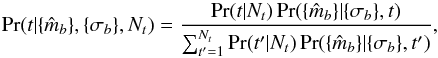 (A.1)where Pr(t | Nt) is the prior probability of the t’th model (i.e., how common this type of astronomical object is) and
  is the marginal likelihood9 that the observed photometry would have been obtained for an object of type t.
Each type is assumed to be specified by a template of model colours (i.e., band-to-band magnitude differences), defined relative to some reference passband B. The colour for template t and band b is denoted cb,t, with cB,t = 0 by construction. The specification of templates by colours means that the source’s (unknown) magnitude in the reference band, mB, must also be included in each model. If this quantity is not of interest (as is the case here), mB can be integrated out to give the marginal likelihood for the t’th type as 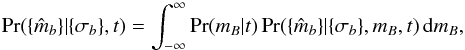 (A.2)where Pr(mB | t) is the prior distribution of mB for objects of the t’th type (and so approximately proportional to their observed number counts) and
  is the likelihood of obtaining the measured data given a value for mB.
Under the assumptions that the measurements in the Nb bands are indepenent and that the variance is additive and normally distributed (in magnitude units10), the likelihood is ![Mathematical equation: \appendix \setcounter{section}{1} \begin{equation} \prob(\data | \noise, \offset_B, t) = \prodband \frac{ \exp\left[- \frac{1}{2} ( \est{m}_\band - \offset_B - c_{\band, t})^2/\sigma_\band^2 \right] } { (2 \pi)^{1/2} \sigma_\band }, \label{equation:lik_1} \end{equation}](/articles/aa/full_html/2015/02/aa24570-14/aa24570-14-eq161.png) (A.3)where mB + cb,t is the predicted b-band magnitude11. Equation (A.3) can be re-written as
(A.3)where mB + cb,t is the predicted b-band magnitude11. Equation (A.3) can be re-written as ![Mathematical equation: \appendix \setcounter{section}{1} \begin{equation} \prob(\data | \noise, \offset_B, t) = \frac{ \exp\left[- \frac{1}{2} \chi^2(\data, \noise, \offset_B, t) \right] } {\prodband (2 \pi)^{1/2} \sigma_\band }, \label{equation:chisq} \end{equation}](/articles/aa/full_html/2015/02/aa24570-14/aa24570-14-eq164.png) (A.4)where
(A.4)where 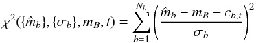 (A.5)is the standard χ2 mis-match statistic. For the purposes of evaluating the integral in Eq. (A.2) it is useful to further rearrange Eq. (A.3) into the form
![Mathematical equation: \appendix \setcounter{section}{1} \begin{eqnarray} &&\prob(\data | \noise, \offset_B, t) = \\\nonumber &&\frac{ \exp\left[ -\frac{1}{2} \chi^2(\data, \noise, \est{\offset}_{B,t}, t) \right] } { \prodband (2 \pi)^{1/2} \sigma_\band } \exp \left\{ -\frac{1}{2} \left[ \frac{ \offset_B - \est{\offset}_{B,t} } {\left(\sumband 1/\sigma_\band^2\right)^{-1/2}} \right]^2 \right\}, \label{equation:lik_2} \end{eqnarray}](/articles/aa/full_html/2015/02/aa24570-14/aa24570-14-eq166.png) (A.6)where
(A.6)where 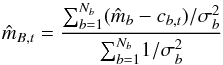 (A.7)is the natural inverse-variance weighted estimate of mB for this combination of source photometry and template, and
  is similarly the minimum value of χ2.
Inserting the above expression for the likelihood into Eq. (A.2) allows the marginal likelihood to be written as
![Mathematical equation: $$ \prob(\data | \noise, t) = \frac{ \exp\left[ -\frac{1}{2} \chi^2(\data, \noise, \est{\offset}_{B,t}, t) \right] } { \prodband (2 \pi)^{1/2} \sigma_\band } $$](/articles/aa/full_html/2015/02/aa24570-14/aa24570-14-eq169.png)
![Mathematical equation: \appendix \setcounter{section}{1} \begin{equation} \label{equation:evidence2} \qquad\;\times \int_{-\infty}^\infty \prob(\offset_B | t) \, \exp \left\{ -\frac{1}{2} \left[ \frac{ \offset_B - \est{\offset}_{B,t} } {\left(\sumband 1/\sigma_\band^2\right)^{-1/2}} \right]^2 \right\} \, \diff \offset_B, \end{equation}](/articles/aa/full_html/2015/02/aa24570-14/aa24570-14-eq170.png) (A.8)illustrating that the goodness of fit and the number counts of this type play quite strongly separated roles in this problem.
(A.8)illustrating that the goodness of fit and the number counts of this type play quite strongly separated roles in this problem.
The classification statistic defined in Sect. 3 comes from adopting a uniform mB prior distribution of the form 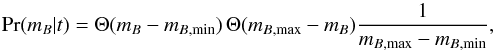 (A.9)where Θ(x) is the Heaviside step function and mB,min and mB,max are taken to be the same for all types (hence the lack of a t subscript). Provided that
  and
and  , the integral in Eq. (A.8) can be approximated analytically to give the marginal likelihood as
![Mathematical equation: \appendix \setcounter{section}{1} \begin{eqnarray} &&\prob(\data | \noise, t) = \nonumber \\ &&\qquad \frac{ \left(\sumband 1/\sigma_\band^2\right)^{-1/2} } {(2 \pi)^{\nband/2 - 1} \left( \prodband \sigma_\band \right)} \frac{ \exp\left[ -\frac{1}{2} \chi^2(\data, \noise, \est{\offset}_t, t) \right]} {\offset_{B,\maximum} - \offset_{B,\minimum}}, \end{eqnarray}](/articles/aa/full_html/2015/02/aa24570-14/aa24570-14-eq177.png) (A.10)where
(A.10)where  is given in Eq. (A.7) and
  is given in Eq. (A.4). Inserting this expression into Eq. (A.1), the posterior probability that the source is of type t becomes
![Mathematical equation: \appendix \setcounter{section}{1} \begin{eqnarray} && \prob(t | \data, \noise, \ntype ) = \nonumber \\ &&\qquad\qquad \frac { \prob(t | \ntype ) \, \exp\left[ -\frac{1}{2} \chi^2(\data, \noise, \est{\offset}_{B,t}, t) \right] } { \sum_{t^\prime=1}^{\ntype} \prob({t^\prime} | \ntype ) \, \exp\left[ -\frac{1}{2} \chi^2(\data, \noise, \est{\offset}_{B,t^\prime}, {t^\prime}) \right] }\cdot \label{equation:final} \end{eqnarray}](/articles/aa/full_html/2015/02/aa24570-14/aa24570-14-eq180.png) (A.11)This probabilistic template matching scheme can be made absolute by classifying a source as being of the type with the maximum posterior probability, which in turn corresponds to the maximum value of the numerator of Eq. (A.11),
(A.11)This probabilistic template matching scheme can be made absolute by classifying a source as being of the type with the maximum posterior probability, which in turn corresponds to the maximum value of the numerator of Eq. (A.11), ![Mathematical equation: \hbox{$\prob(t | \ntype ) \, \exp[- \chi^2(\data, \noise, \est{\offset}_{B,t}, t)/2]$}](/articles/aa/full_html/2015/02/aa24570-14/aa24570-14-eq181.png) . If the relative numbers of the different source types are comparable (or if the templates have very distinct colours, relative to the photometric noise) then the differences in the priors can be neglected, in which case a source would be classified as being of the type t which yields the minimum value of . This is the approach taken in Sect. 2.
. If the relative numbers of the different source types are comparable (or if the templates have very distinct colours, relative to the photometric noise) then the differences in the priors can be neglected, in which case a source would be classified as being of the type t which yields the minimum value of . This is the approach taken in Sect. 2.
All Tables
All Figures
|
Fig. 1 i − z colour vs. spectral sub-type for MLT dwarfs in the UKIDSS LAS DR10 footprint. The error bars plotted show the random photometric errors. The fitted curve provides the template colours listed in Table 1. In making the fit, a colour error of 0.07 mag. (i.e. 0.05 mag. in each band) is added in quadrature to the random photometric errors to account for intrinsic scatter in the colours. The very large errors in the T dwarf regime mean that the curve is poorly defined in this region, as discussed in the text. The vertical scale is the same as in Fig. 2. The outlying blue T0 dwarf is discussed in Sect. 3.2. All photometry is on the Vega system. |
| In the text | |
|
Fig. 2 Colours z − Y, Y − J, J − H, H − K, K − W1, W1 − W2 vs. spectral sub-type for MLT dwarfs in the UKIDSS LAS DR10 footprint. The errorbars plotted show the random photometric errors. The fitted curve provides the template colours listed in Table 1. In making the fit, a colour error of 0.07 mag. (i.e. 0.05 mag. in each band) is added in quadrature to the random photometric errors to account for intrinsic scatter in the colours. The vertical scale is the same as in Fig. 1. All photometry is on the Vega system. |
| In the text | |
|
Fig. 3 Colour curves from Figs. 1 and 2 plotted in a single figure in order to compare the relative usefulness of different colours in classifying different spectral types in the LT sequence. |
| In the text | |
|
Fig. 4 Uncertainties of the fits of the colour polynomials as a function of spectral type. With the exception of the i − z and K − W1 curves the uncertainties are significantly smaller than the intrinsic scatter (marked by the dashed line). |
| In the text | |
|
Fig. 5 χ2 (computed from Eq. (2)) against spectral type, in the classification of four known L and T dwarfs, as follows: SDSS J0149+0016 (L0, J = 17.18±0.03), 2MASS J1407+1241 (L5, J = 15.33±0.004), ULAS J1516+0259 (T0, J = 16.88±0.02), and ULAS J1417+1330 (T5, J = 16.77±0.01). In each case the χ2 curves show no degeneracies, and are sharp, indicating accurate classification (quantified in Sect. 3.2). |
| In the text | |
|
Fig. 6 Contour plot illustrating sensitivity to detection of unresolved binaries. The axes correspond to the two components of a binary. The contours plot the improvement in χ2 of a binary dwarf solution over the best single dwarf solution. |
| In the text | |
|
Fig. 7 Comparison of photo-type classification vs. spectroscopic classification for the 189 known L and T dwarfs from DwarfArchives, as well as 111 late M stars. Classifications were computed to the nearest half spectral sub-type. Because the classifications are quantised, small offsets have been added in order to show all the points. The dashed lines mark misclassification by four spectral sub-classes. The three outliers marked by diamonds are discussed in the text. |
| In the text | |
|
Fig. 8 SED of the source SDSS J1030+0213 compared to the photo-type classification of L4 (black line), and the spectroscopic classification of L9.5 (red line). The upper plot uses flux (fλ), normalised to J, and the lower plot uses magnitudes. |
| In the text | |
|
Fig. 9 SED of the source 2MASS J1542-0045 compared to the photo-type classification of L2 (black line), and the spectroscopic classification of L7 (red line). The upper plot uses flux (fλ), normalised to J, and the lower plot uses magnitudes. |
| In the text | |
|
Fig. 10 SED of the source ULAS J2304+1301 compared to the photo-type classification of L3.5 (black line), and the spectroscopic classification of T0 (red line). The upper plot uses flux (fλ), normalised to J, and the lower plot uses magnitudes. |
| In the text | |
|
Fig. 11 SpeX spectra of eight sources used to estimate the accuracy of photo-type. The sources are classified as L1 (ULAS J0026+0632), L1 (ULAS J0109+0625), L8 (ULAS J0246+0156), L1 (ULAS J0741+2316), L1 (ULAS J0849+2739), T3 (ULAS J0915+0531), L9.5 (ULAS J1029+0620), and M9 (ULAS J1053+0452), by comparison against the spectroscopic standards listed in Table 3. The standard closest in spectral type is also shown for each source. |
| In the text | |
|
Fig. 12 Estimated accuracy rms of the photo-type classification for sources of J = 16.0 (red curve) and J = 17.5 (black curve) based on classification of synthetic data. |
| In the text | |
Current usage metrics show cumulative count of Article Views (full-text article views including HTML views, PDF and ePub downloads, according to the available data) and Abstracts Views on Vision4Press platform.
Data correspond to usage on the plateform after 2015. The current usage metrics is available 48-96 hours after online publication and is updated daily on week days.
Initial download of the metrics may take a while.