| Issue |
A&A
Volume 574, February 2015
|
|
|---|---|---|
| Article Number | A16 | |
| Number of page(s) | 7 | |
| Section | Stellar structure and evolution | |
| DOI | https://doi.org/10.1051/0004-6361/201424245 | |
| Published online | 16 January 2015 | |
Constraining the shaping mechanism of the Red Rectangle through the spectro-polarimetry of its central star
1 Instituto de Astrofísica de Canarias, 38205 La Laguna, Tenerife, Spain
e-mail: This email address is being protected from spambots. You need JavaScript enabled to view it.
2 Departamento de Astrofísica, Universidad de La Laguna, 38205 La Laguna, Tenerife, Spain
3 Dipartimento di Fisica e Astronomia, Universitá di Catania, Sezione Astrofisica, via S. Sofia 78, 9512, Catania, Italy
Received: 21 May 2014
Accepted: 12 October 2014
Abstract
We carried out high-sensitivity spectro-polarimetric observations of the central star of the Red Rectangle protoplanetary nebula with the aim of constraining the mechanism that gives its biconical shape. The stellar light of the central binary system is linearly polarised since it is scattered on the dust particles of the nebula. Surprisingly, the linear polarisation in the continuum is aligned with one of the spikes of the biconical outflow. Also, the observed Balmer lines, as well as the Ca ii K lines, are polarised. These observational constraints are used to confirm or reject current theoretical models for the shaping mechanism of the Red Rectangle. We propose that the observed polarisation is not very likely to be generated by a uniform biconical stellar wind. Also, the hypothesis of a precessing jet does not completely match observations since it requires a larger aperture jet than for the nebula.
Key words: polarization / stars: AGB and post-AGB / planetary nebulae: individual: Red Rectangle
© ESO, 2015
1. Introduction
The Red Rectangle is a protoplanetary nebula with a biconical shape extending away from the central object HD 44179. The central object is known to be a single line spectroscopic binary system composed of a secondary star that accretes material from the primary post-AGB star forming an accretion disc. The nature of the secondary star is still a matter of debate. Men’shchikov et al. (2002) propose that it is a white dwarf although Waelkens et al. (1996) and Witt et al. (2009) consider that it is a low-mass main sequence star. The accretion disc of the secondary star is supposed to accelerate a secondary wind along its polar axis forming a jet.
The central stellar system is obscured by an optically thick torus and is observed from the scattering of the light in dust particles. This scattering produces two bright hyperbolic arcs with the southernmost one brighter than the northernmost one. The reason one lobe is brighter than the other is still not known (Cohen et al. 2004), but it is possibly related to the scattering physics and/or the distribution of dust particles in both hemispheres. The inclined torus obscures a larger portion of the northern hemisphere and the scattered light comes from larger distances from the central system. Expanding discs around post-AGB stars are fairly common but the Red Rectangle is the only object with a rotating disc (Bujarrabal et al. 2005) plus the expected expansion (Bujarrabal et al. 2013).
Two main physical mechanisms have been proposed to explain the shape of most bipolar nebulae. The most popular one states that in a close binary system angular momentum provides a natural preferred axis (Morris 1981, 1987). A second mechanism involves the presence of a mostly dipolar magnetic field where the matter can be collimated at the poles of the field. However, at present, a clear detection of such fields has not been found (Leone et al. 2011; Jordan et al. 2012).
To shape the Red Rectangle, two main scenarios have been proposed: one that assumes that the secondary wind is a well collimated jet inclined by 30° (with respect to the symmetry axis of the nebula) that precesses every 17.6 years (Soker 2005; Velázquez et al. 2011), and another one that assumes a bipolar outflow (or wide jet) with the same opening as the nebula (Morris 1981, 1987; Soker 2000; Thomas et al. 2013; Icke 1981; Koning et al. 2011). Spectro-polarimetry is a valuable tool that allows us to differentiate between the two scenarios. The physical mechanism that shapes this nebula must explain the observed light polarisation. Here we present linear spectro-polarimetry of the central stellar system of the Red Rectangle. We compare these observations with the theoretical expected linear polarisation from different mechanisms proposed to give the biconical shape to this object.
2. Observations and data reduction
The data consist of full-vector spectro-polarimetry of the central binary system of the Red Rectangle (HD 44179) at blue wavelengths between 365 and 510 nm, approximately. The observations were taken on September 4 2012 using the FORS2 polarimeter (Appenzeller et al. 1998) attached to the Very Large Telescope (VLT) at Cerro Paranal. We used the 1200B grism and a slit width of 0.5′′ to achieve a spectral sampling of 0.036 nm at 450 nm. The total integration time for each Stokes parameter was 8 min, which allowed us to obtain a polarimetric signal-to-noise ratio of about 1250. The slit was oriented 55° from the celestial north to the east, close to the parallactic angle at that moment. The inclination of the slit does not introduce any bias in the observed polarisation since the central object HD 44179is unresolved. As seen in Fig. 7 in Cohen et al. (2004), the maximum of the scattered light of the central object is enclosed in about ~0.2″.
We focus on the study of the linear polarisation that carries information about the unresolved geometry of the central system. The circular polarisation pattern, which allows the detection of magnetic fields if present, has been analysed by our group (Asensio Ramos et al. 2014; Leone et al. 2014), showing that there is no clear evidence of any organized magnetic field in the central binary system of the Red Rectangle.
The FORS2 polarimeter is composed of two retarders (a quarter wave plate and a half wave plate), and a beam splitter (the analyser). For convenience, we rotated the retarders to obtain the fractional polarisation (the polarisation relative to the intensity) according to the following modulation scheme in one of the beams produced by the analyzer: FI + Fj, FI − Fj, FI − Fj, FI + Fj, with j = Q,U. The orthogonal state of polarisation for each modultation step is recorded simultaneously in the other beam position. With the available measurements, we computed the fractional polarisation Fj/FI as (Bagnulo et al. 2009): 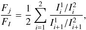 (1)where I1 and I2 denote the intensity measured in each one of the beams, while index i represents each one of the modulation steps. This modulation scheme allows us to efficiently correct, to first order, the flatfield, differential defocusing, and different seeing conditions during the different exposures. An additional advantage is that it allows us to compute the null spectra (Donati et al. 1997), which gives an idea of the residual errors in the data:
 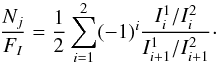 (2)Given that the spectrograph is not perfectly stabilised, we need to re-align the spectra in wavelength for each modulation state. We do this by using a calibration arc lamp exposure. To avoid possible spurious signals (Bagnulo et al. 2009), we use only a single wavelength calibration for all the modulation states. Additionally, given that the spectra are not aligned with the borders of the detector, we use the flatfield image to compute the position of the beams at each wavelength. Once they are aligned, we integrate each beam along the slit direction and then use Eq. (1) to obtain the fractional polarisation. The reason for doing the demodulation in this order is that the error propagation is simpler and more advantageous.
In general, it is quite difficult to know a-priori which of the two beams on the detector contains FI + Fj or FI − Fj. The reason is that this requires us to know exactly the position of the axis of the analyser, which is not the case in many instruments. If one switches both beams, the resulting polarisation will be rotated by 90°. To calibrate the two beams, we observe a linear polarisation standard star whose polarisation degree and angle are known. This observation can also help to estimate if there is any induced instrumental polarisation. In our observing run we observed the Hiltner 652 star, which has a degree of polarisation of 5.72 ± 0.02% and a polarisation angle of 179.8±0.1° as observed with a filter in the Johnson B band1. Given that these are broad band calibrations, we computed from our data the degree and angle of polarisation from the integrated Stokes FQ and FU wigthed by the Johnson B filter transmission, B(λ), as 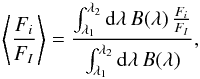 (3)where the polarisation degree and angle are defined as
 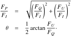 (4)We obtain ⟨ FP/FI ⟩ = 5.9 ± 0.6% and θ = 0.0 ± 0.5°, which are compatible with the tabulated values inside the error bars. This means that the instrumental polarisation is negligible and that the instrument rotation is properly considered in the data reduction.
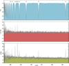 |
Fig. 1 From top to bottom: blue spectra of the intensity flux, polarisation degree, and polarisation angle of the central star of the Red Rectangle. The mode of the FP/FI distribution is the standard deviation of Stokes FQ and FU parameters, which means that if both FQ and FU are zero, the FP/FI will have a value of 0.08%. |
Given that we are dealing with absolute polarimetry, it is important to check the influence of interstellar polarisation along the line-of-sight. Reese & Sitko (1996) estimate (using field stars) that the degree of polarisation of the interstellar component is at most 0.2%. Since they observe a degree of polarisation of 2.2% in the continuum, this means that only ~9% of their observed continuum polarisation in the Red Rectangle can be attributed to interstellar polarisation. Unfortunately, they do not compute the estimated rotation angle produced by the interstellar medium, so we try to provide an upper limit to this effect. The influence of the interstellar polarisation on the polarisation of the object is given by 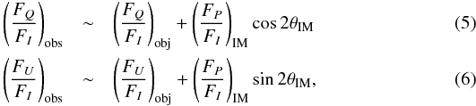 where the subindex “obs” represents the observed Stokes parameters, i.e., the addition of the polarisation coming from the object (labelled with “obj“) and the polarisation coming from the interstellar medium (labelled with “IM”). This formula is a good approximation if the polarisation of the interstellar medium is low. Also, if this happens, we can substitute the object polarisation (that is unknown) with the observed one. Then, to first order, we have
 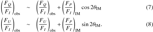 Assuming the value of Reese & Sitko (1996) for the polarisation degree of 0.2% and using all possible values of θIM, we find that the maximum influence on the polarisation angle inferred from FQ/FI and FU/FI is only ± 4°.
Our data offer another possibility to compute an upper limit to the polarisation of the interstellar medium. The Ca ii H line at 3968.5 Å, a transition between Jup = Jlow = 1 / 2 levels, cannot be polarised by scattering processes2. Therefore, all the photons emitted in the Ca ii H line are not polarised, so that the degree of polarisation will tend to zero. Consequently, if the degree of polarisation of the Red Rectangle at the Ca ii H line is not zero, then the observed absolute polarisation is coming from the interstellar medium. However, in general, the emission of spectral lines is not enough to fully depolarise (except for some very strong lines), and the polarisation we observe in the Ca ii H line (0.8%) is an upper limit for the polarisation of the interstellar medium. The same applies to the angle of polarisation in this line. Using the previous conditions, a very conservative maximum error in the polarisation angle is ~ ± 17°. We conclude that the measured angle of polarisation of the Red Rectangle is well defined.
3. Results
Figure 1 displays the observed intensity flux spectrum (upper panel), the polarisation degree (middle panel), and angle (lower panel). Contrary to the polarisation degree, which does not depend on the chosen reference system used to measure the Stokes parameters, the polarisation angle does depend on the reference system. We define θ = 0° at the celestial N-S direction (for an easier comparison with Reese & Sitko 1996), increasing toward the east. The polarisation angle does not depend on the intensity flux.
The continuum is polarised at ~1.4% with an angle of ~ 45° with respect to the celestial N. Given that the symmetry axis of the conical structure is inclined 10° with respect to the celestial N, the polarisation makes an angle of 35° with respect to the symmetry axis of the nebula, coinciding, surprisingly, with one of the spikes of the nebula. Reese & Sitko (1996), 17.8 years before our observation, measured a continuum degree of polarisation of 2.2%. The measured polarisation angle was ~43°, very similar to our result. It is likely that the 50% difference between the values of the degree of polarisation at the continuum is due to the different sensitivity of the two data sets, with our data being much more sensitive. However, we need more observations to check wether this variation is real or not.
Observations of the continuum linear polarisation of the outer parts of the Red Rectangle have been previously reported by Perkins et al. (1981) in the red (6100−7500 Å) and blue wavebands (4000−5000 Å). In both cases, they observe the polarisation angle following a centrosymmetric pattern, as expected from the scattering of the light from the central object in the walls of the bicones. The same result is found by Gledhill et al. (2009) in the near infrared. The compatibility of these two works and our result is a matter of spatial scales. If the physical mechanism that breaks the symmetry plays a major role in the central parts of the nebula (has a small spatial extent of about 1′′), the polarisation we measure is an effect of this symmetry breaking. If we move to the outer nebula, the linear polarisation is blind to this smaller scale mechanism and reflects the symmetry of the large scale nebula. However, in Fig. 1 of Gledhill et al. (2009), the polarisation in the nbL filter (the one that better “resolves” the central parts of the nebula) shows polarisation angles that are not centrosymmetric (at about ~60°) at 1′′ surrounding the central object.
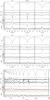 |
Fig. 2 Close look to the Balmer lines and the Ca ii K line. From top to bottom, the spectra of the intensity flux, the flux of the Stokes Q and U parameters in terms of the intensity flux, the polarisation degree, and the polarisation angle. The shadowed areas represent the 2-sigma confidence level for these derived quantities. |
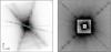 |
Fig. 3 Backgroud image of the Red Rectangle protoplanetary nebula as seen in the red (left panel; taken from Koning et al. 2011) and in the blue (right panel; taken from Cohen et al. 2004). The lines represent the direction of the polarisation of the continuum (red), the Balmer lines (blue) and the Ca ii K line (green). The size of the lines represents the degree polarisation with respect to the continuum value. |
Figure 2 shows a closer look at the intensity flux, Stokes Q and U parameters, and total polarisation and angle for the Balmer lines and the Ca ii K line. The shadowed areas in polarisation and in the polarisation angle represent the 2σ uncertainty levels produced by photon noise using the formula from Bagnulo et al. (2009). Most of the Balmer lines, notably Hβ, Hγ, Hϵ , Hζ, and Hη have linear polarisations that are clearly rotated with respect to the continuum by 20° − 45°. It is interesting to point out that the scattering process for the lines Hϵ, Hδ, Hγ, and Hβ has only modified the angle and not the polarisation degree. The Hϵ line is blended with the Ca ii H line, which cannot be polarised, so it can be affected by an artificial reduction of the polarisation angle. The Hδ line, however, is just slightly rotated with respect to the continuum (~ 5° − 10°), in contrast to the rest of the Balmer lines. The Ca ii K line presents the highest degree of polarisation and also the largest angle (~ 85°). Given that the transmission of the isntrumental system below 380 nm is poor, we prefer not to conclude anything until it is observed with a better signal-to-noise ratio, even though some features are seen. Unfortunately, our data coverage does not reach Hα, but we point out that Reese & Sitko (1996) observe an excess of polarisation in this line of 7.9 ± 0.6% with an polarisation angle of 102 ± 2° with respect to celestial north.
Figure 3 displays the directions of the polarisation of the continuum, the Balmer lines, and the Ca ii K line superimposed on the image of the Red Rectangle proto-PN as observed in the red wavelengths (left panel) and in the blue (right panel). The nebula looks more spherical in the blue wavelengths and has a smaller size (Perkins et al. 1981; Cohen et al. 2004). As stated above, the continuum polarisation is aligned with one of the spikes of the proto-PN. The linear polarisation of the spectral lines are rotated with respect to this direction by 20° − 45° in the eastern direction, Hζ presenting a linear polarisation that is almost perpendicular to the spike of the proto-PN that is not aligned with the linear polarisation of the continuum.
4. Discussion
That we detect non-zero continuum polarisation and a rotation of the angle with respect to the equatorial plane can only be explained if there is a certain degree of symmetry breaking in the system. Several options are available, and we discuss them in the light of the observations. The most obvious one is that the symmetry breaking is related to the binarity. Using the information provided in Thomas et al. (2013) for the ephemerids of the binary system, the observations of Reese & Sitko (1996) were carried out at phase φ = 0.36, while ours were done at phase φ = 0.84, almost in opposite orbital phases. The propagation of the error on the period estimation of the binary system might make the two phases compatible. However, recently Witt et al. (2009) have confirmed a period of 318 ± 1 day, i.e., an error of only 0.3%. Therefore, we have to conclude that the orbital phases of our observations and those from Reese & Sitko (1996) are completely different. Considering Rayleigh scattering, we expect a 1% modulation of the degree of polarisation between the periastron and the apastron. Unfortunately, this is still not detectable considering our observational capabilities.
The presence of a thick dusty torus (Bujarrabal & Alcolea 2013) and the fact that it is slightly tilted (see Fig. 4) is another source of symmetry breaking. The dusty disc allows us to view the light of the binary star only by scattering processes. As can be seen in Fig. 4, the radius of the disc occults regions closer than ~211 AU to the binary star in the upper cone and in regions closer than ~50 AU in the lower cone. Since both the density of scatterers and the radiation field decrease from the central binary system, we can safely consider that the scattering is fundamentally coming from the lower half of the circunbinary disc, i.e., at a distance of ~50 AU as measured from the equatorial plane of the binary system. In the absence of any other mechanism and for reasons of symmetry, this would generate linear polarisation that should be parallel or perpendicular to the symmetry axis of the nebula. To explain the rotation of ~45° with respect to the celestial N, we need to invoke other symmetry-breaking mechanisms.
In light of the previous considerations, we can think of two mechanisms that are possible to explain the observations. The two possibilities are depicted in Fig. 5. The first one is that the scattering takes place in the bipolar flow (case a, see upper panel of Fig. 5). The second one is that it happens in a dense collimated jet (case b). In case a), if the binary system is located at the centre of the nebula, we expect the polarisation of the continuum to be in the equatorial plane of the torus-binary system (e.g. Daniel 1982; Cohen & Schmidt 1982; Harries 1996). To produce the observed rotation that produces polarisation parallel to the spike of the nebula, the binary system would have to be decentred by d = 70 AU(taking the geometric considerations shown in Fig. 4 into account). Considering that the star separation is always smaller than 1 AU Thomas et al. (2013) and that the inner radius of the torus is 14 AU (Men’shchikov et al. 2002), we find that a bipolar flow alone cannot explain the observed continuum polarisation in the Red Rectangle. Additionally, if a bipolar flow is taking place, we expect the polarisation to be modulated by the orbital period of the binary system. Nevertheless, both Reese & Sitko (1996) and our observations, presenting very different phases, show the same angle of polarisation.
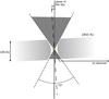 |
Fig. 4 Schematic drawing of the unresolved center of the Red Rectangle, which is inclined by 5° with respect to the line of sight (LOS). The plane of the sky is perpendicular to the sheet, and the line-of-sight is represented in red. The spikes that are observed in the red are represented as dashed black lines. The central binary system is represented by an orange circle (the AGB) and an orange rectangle (the accretion disc). The light grey area around the central system is the optically thick torus, which has an outer radius estimation of 1850 AU, an inner radius (the cavity of the binary system) of 14 AU, and a thickness of about 100 AU (Bujarrabal & Alcolea 2013). The dark grey area represents the area of the Red Rectangle is hidden to the observer by the circunbinary disc. The disc is so large that about 161 AU height as measured from the plane of the binary system is obscured. |
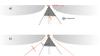 |
Fig. 5 Possible scattering mechanisms producing the polarisation in the continuum that we observe. We only display one cone (the lower cone but mirrored with respect to the orbital plane) since the scattered light is mostly generated there (i.e., the larger the distance from the central object, the lower the density and the intensity of the radiation field). Grey dots represent the scatterers. The spikes of the nebula are traced in black dashed lines, the central system is represented in orange, the horizontal line representing the accretion disc. The observed linear polarisation is displayed in red. Case a) depicts the scattering produced at all points of the cone (i.e., the wide jet mechanism). The expected theoretical polarisation in this case is represented as a short-dashed orange line. Case b) displays the case where the scattering occurs at the aperture θ that gives a polarisation that is compatible with the observed one. |
In case b), where we assume a dense collimated jet, the scattering will take place mainly at the jet. Consequently, the polarisation will be perpendicular to the scattering plane formed by the jet and the line of sight. According to this picture (see lower panel of Fig. 5) and our measurements, we can estimate that the opening angle of this jet should be ~55°. If the jet is precessing, we would get a biconical structure with a full aperture of 110°. The full aperture of the biconical walls of the Red Rectangle measured from imaging data vary from 40° close to the central source to 80° at larger distances (Cohen et al. 2004). On average, the opening angle we infer is 20° larger than the semi-aperture of the nebula (measured from the symmetry axis to the nebula) and 25° larger than the expected aperture of a precessing jet computed by Velázquez et al. (2011). In spite of this difference, we note that the Red Rectangle has a larger aperture (about 90°) as observed in polarised light at optical wavelengths (see Fig. 2 in Perkins et al. 1981). Also, it is important to note that our considerarions are purely geometric in nature and that any radiative transfer effect on the spectral lines can easily compensate for these differences in the polarisation angle. A precessing jet puts constraints on the modulation of the observed polarisation with the rotational period. Unfortunately, there have been 17.8 years since the observations of Reese & Sitko (1996), a similar period to the one needed in Velázquez et al. (2011) to shape the Red Rectangle with a precessing jet (17.6 years). In order to confirm or discard the hypothesis of a precessing jet, we plan to spectro-polarimetrically survey the Red Rectangle in forthcoming years.
A feature that we find intriguing is that the linear spectro-polarimetry of the Red Rectangle reveals that the hydrogen Balmer lines, and the doubly ionized Ca K line are polarised with respect to the continuum, and are additionally rotated with respect to the continuum by different amounts depending on the spectral line. Only resonant scattering, i.e., polarisation in spectral lines, can produce a rotation of the polarisation angle. Also, that the Ca ii K is the most polarised line and is, in turn, the most shallow line in the intensity spectrum reinforces the assumption that the observed signals are produced by scattering in spectral lines. Scattering polarisation in spectral lines is induced by the presence of population imbalances and quantum coherences (atomic level polarisation) between magnetic sublevels caused by the absorption of anisotropic radiation (e.g., Landi degl’Innocenti & Landolfi 2004), which is mainly controlled by the amount of anisotropy of the radiation field. Any other mechanism (two different offset sources for the continuum and the spectral lines, or stray light) cannot explain the observed polarisation angles and would hardly polarise spectral lines (in general, spectral lines would appear as a depolarisation of the continuum).
The rotation of resonance scattering polarisation with respect to the symmetry axis of the nebula indicates that there is another preferred axis that breaks the apparent symmetry of the nebula. Several mechanisms can produce such a rotation. A magnetic field naturally imposes another preferred axis, modifying the polarisation signals leading to a rotation of the plane of polarisation through the Hanle effect. To get such a rotation, the magnetic field strength should be in the so-called Hanle critical field, which is ~ 1−100 G for the hydrogen lines (e.g., Štěpán & Trujillo Bueno 2011) and ~ 1−120 G for the Ca ii K line. Under the assumption of a dipolar magnetic field in the central region of the Red Rectangle, we expect the magnetic field strength to decrease as the cube of the distance. Therefore, the Hanle effect has to be discarded as a source of the rotation of the linear polarisation because, in order to have Hanle effect at ~50 AU, the magnetic field strength at 1 AU would have to be 0.1−10 MG.
Another way of producing a rotation of the polarisation is by optical depth effects, which has been proposed in the past to explain polarimetric observations of SiO masers (Asensio Ramos et al. 2005). The specific orientation of the polarisation depends on the balance between radiation tending to escape along the flow (giving polarisation perendicular to the symmetry axis of the nebula) or mainly along the orbital plane of binary star (giving polarisation parallel to the symmetry axis of the nebula). Local density accumulations produce a modification of the anisotropy of the radiation field that can lead to local rotations of the polarisation of the emitted radiation. Additionally, a large velocity gradient along a certain direction produces an enhancement of the anisotropy along this direction via the Doppler brightening effect (Carlin et al. 2012). This could be related to the inherent mass loss of the star.
The observed angle of polarisation at the blue continuum reveals that a wide jet is not likely to be shaping the Red Rectangle (cf. Morris 1981, 1987; Soker 2000; Thomas et al. 2013; Icke 1981; Koning et al. 2011). A large mass inhomogeineity (like a collimated jet Soker 2005; Velázquez et al. 2011) could explain the shape of the nebula if it is orientated along a position angle of about 55°. By gathering more data, our future efforts will be toward understanding the physical mechanisms that generate the polarisation properties of this protoplanetary nebula.
Under anisotropic pumping, the populations of the mJ> 0 and mJ< 0 magnetic sublevels are not the same. The Ca ii H line has Jup = Jlow = 1 / 2, and almost 100% of the Ca ii has no hyperfine structure. Then, it can never have population imbalances between its magnetic sublevels and then produce linear polarisation in the emission process.
Acknowledgments
We are very grateful to S. Bagnulo for helpful advice on the data reduction and to an anonymous referee whose comments have strengthened the conclusions of this work. Support by the Spanish Ministry of Economy and Competitiveness through projects AYA2010–18029 (Solar Magnetism and Astrophysical Spectro-polarimetry) and Consolider-Ingenio 2010 CSD2009-00038 are gratefully acknowledged. A.A.R. also acknowledges financial support through the Ramón y Cajal fellowships.
References
- Appenzeller, I., Fricke, K., Fürtig, W., et al. 1998, The Messenger, 94, 1 [NASA ADS] [Google Scholar]
- Asensio Ramos, A., Landi Degl’Innocenti, E., & Trujillo Bueno, J. 2005, ApJ, 625, 985 [NASA ADS] [CrossRef] [Google Scholar]
- Asensio Ramos, A., Martinez Gonzalez, M. J., Manso Sainz, R., Corradi, R. L. M., & Leone, F. 2014, ApJ, 787, 11 [Google Scholar]
- Bagnulo, S., Landolfi, M., Landstreet, J. D., et al. 2009, PASP, 121, 993 [NASA ADS] [CrossRef] [Google Scholar]
- Bujarrabal, V., & Alcolea, J. 2013, ApJ, 552, 116 [Google Scholar]
- Bujarrabal, V., Castro-Carrizo, A., Alcolea, J., & Neri, R. 2005, A&A, 441, 1031 [NASA ADS] [CrossRef] [EDP Sciences] [Google Scholar]
- Bujarrabal, V., Castro-Carrizo, A., Alcolea, J., et al. 2013, A&A, 557, L11 [NASA ADS] [CrossRef] [EDP Sciences] [Google Scholar]
- Carlin, E. S., Manso Sainz, R., Asensio Ramos, A., & Trujillo Bueno, J. 2012, ApJ, 751, 5 [NASA ADS] [CrossRef] [Google Scholar]
- Cohen, M., & Schmidt, G. D. 1982, ApJ, 259, 693 [NASA ADS] [CrossRef] [Google Scholar]
- Cohen, M., van Winckel, H., Bond, H. E., & Gull, T. R. 2004, AJ, 127, 2362 [NASA ADS] [CrossRef] [Google Scholar]
- Daniel, J.-Y. 1982, A&A, 111, 58 [NASA ADS] [Google Scholar]
- Donati, J.-F., Semel, M., Carter, B. D., Rees, D. E., & Collier Cameron, A. 1997, MNRAS, 291, 658 [NASA ADS] [CrossRef] [MathSciNet] [Google Scholar]
- Gledhill, T. M., Witt, A. N., Vijh, U. P., & Davis, C. J. 2009, MNRAS, 392, 1217 [NASA ADS] [CrossRef] [Google Scholar]
- Harries, T. J. 1996, A&A, 315, 499 [NASA ADS] [Google Scholar]
- Icke, V. 1981, ApJ, 247, 152 [NASA ADS] [CrossRef] [Google Scholar]
- Jordan, S., Bagnulo, S., Werner, K., & O’Toole, S. J. 2012, ApJ, 542, 64 [NASA ADS] [CrossRef] [Google Scholar]
- Kemp, J. C., Macek, J. H., & Nehring, F. W. 1984, ApJ, 278, 863 [NASA ADS] [CrossRef] [Google Scholar]
- Koning, N., Kwok, S., & Steffen, W. 2011, ApJ, 740, 27 [NASA ADS] [CrossRef] [Google Scholar]
- Landi degl’Innocenti, E., & Landolfi, M. 2004, Polarization in Spectral Lines (Kluwer Academic Publishers) [Google Scholar]
- Leone, F., Martínez González, M. J., Corradi, R. L. M., Privitera, G., & Manso Sainz, R. 2011, ApJ, 731, L33 [NASA ADS] [CrossRef] [Google Scholar]
- Leone, F., Corradi, R. L. M., Martínez González, M. J., Asensio Ramos, A., & Manso Sainz, R. 2014, A&A, 563, A43 [NASA ADS] [CrossRef] [EDP Sciences] [Google Scholar]
- López Ariste, A., Casini, R., Paletou, F., et al. 2005, ApJ, 621, L145 [NASA ADS] [CrossRef] [Google Scholar]
- Martínez González, M. J., Asensio Ramos, A., Manso Sainz, R., Beck, C., & Belluzzi, L. 2012, ApJ, 759, 16 [NASA ADS] [CrossRef] [Google Scholar]
- Men’shchikov, A. B., Schertl, D., Tuthill, P. G., Weigelt, S. J., & Yungelson, L. R. 2002, A&A, 393, 867 [NASA ADS] [CrossRef] [EDP Sciences] [Google Scholar]
- Morris, M. 1981, ApJ, 249, 572 [NASA ADS] [CrossRef] [Google Scholar]
- Morris, M. 1987, PASP, 99, 1115 [NASA ADS] [CrossRef] [Google Scholar]
- Perkins, H. G., Scarrott, S. M., Murdin, P., & Bingham, R. G. 1981, MNRAS, 196, 635 [NASA ADS] [Google Scholar]
- Reese, M. D., & Sitko, M. L. 1996, ApJ, 467, L105 [NASA ADS] [CrossRef] [Google Scholar]
- Soker, N. 2000, A&A, 357, 557 [NASA ADS] [Google Scholar]
- Soker, N. 2005, AJ, 129, 947 [NASA ADS] [CrossRef] [Google Scholar]
- Štěpán, J., & Trujillo Bueno, J. 2011, ApJ, 732, 80 [NASA ADS] [CrossRef] [Google Scholar]
- Thomas, J. D., Witt, A. N., Aufdenberg, J. P., et al. 2013, MNRAS, 430, 1230 [NASA ADS] [CrossRef] [Google Scholar]
- Velázquez, P. F., Steffen, W., Raga, A. C., Haro-Corzo, S., & Esquivel, A. 2011, ApJ, 734, 57 [NASA ADS] [CrossRef] [Google Scholar]
- Waelkens, C., van Winckel, C., Waters, L. B. F. M., & Bakker, E. J. 1996, A&A, 314, L17 [NASA ADS] [Google Scholar]
- Witt, A. N., & Vijh, U. P. 2004, ASP Conf. Ser., 309, 115 [Google Scholar]
- Witt, A. N., Vijh, U. P., Hobbs, L. M., et al. 2009, ApJ, 693, 1946 [NASA ADS] [CrossRef] [Google Scholar]
All Figures
|
Fig. 1 From top to bottom: blue spectra of the intensity flux, polarisation degree, and polarisation angle of the central star of the Red Rectangle. The mode of the FP/FI distribution is the standard deviation of Stokes FQ and FU parameters, which means that if both FQ and FU are zero, the FP/FI will have a value of 0.08%. |
| In the text | |
|
Fig. 2 Close look to the Balmer lines and the Ca ii K line. From top to bottom, the spectra of the intensity flux, the flux of the Stokes Q and U parameters in terms of the intensity flux, the polarisation degree, and the polarisation angle. The shadowed areas represent the 2-sigma confidence level for these derived quantities. |
| In the text | |
|
Fig. 3 Backgroud image of the Red Rectangle protoplanetary nebula as seen in the red (left panel; taken from Koning et al. 2011) and in the blue (right panel; taken from Cohen et al. 2004). The lines represent the direction of the polarisation of the continuum (red), the Balmer lines (blue) and the Ca ii K line (green). The size of the lines represents the degree polarisation with respect to the continuum value. |
| In the text | |
|
Fig. 4 Schematic drawing of the unresolved center of the Red Rectangle, which is inclined by 5° with respect to the line of sight (LOS). The plane of the sky is perpendicular to the sheet, and the line-of-sight is represented in red. The spikes that are observed in the red are represented as dashed black lines. The central binary system is represented by an orange circle (the AGB) and an orange rectangle (the accretion disc). The light grey area around the central system is the optically thick torus, which has an outer radius estimation of 1850 AU, an inner radius (the cavity of the binary system) of 14 AU, and a thickness of about 100 AU (Bujarrabal & Alcolea 2013). The dark grey area represents the area of the Red Rectangle is hidden to the observer by the circunbinary disc. The disc is so large that about 161 AU height as measured from the plane of the binary system is obscured. |
| In the text | |
|
Fig. 5 Possible scattering mechanisms producing the polarisation in the continuum that we observe. We only display one cone (the lower cone but mirrored with respect to the orbital plane) since the scattered light is mostly generated there (i.e., the larger the distance from the central object, the lower the density and the intensity of the radiation field). Grey dots represent the scatterers. The spikes of the nebula are traced in black dashed lines, the central system is represented in orange, the horizontal line representing the accretion disc. The observed linear polarisation is displayed in red. Case a) depicts the scattering produced at all points of the cone (i.e., the wide jet mechanism). The expected theoretical polarisation in this case is represented as a short-dashed orange line. Case b) displays the case where the scattering occurs at the aperture θ that gives a polarisation that is compatible with the observed one. |
| In the text | |
Current usage metrics show cumulative count of Article Views (full-text article views including HTML views, PDF and ePub downloads, according to the available data) and Abstracts Views on Vision4Press platform.
Data correspond to usage on the plateform after 2015. The current usage metrics is available 48-96 hours after online publication and is updated daily on week days.
Initial download of the metrics may take a while.