| Issue |
A&A
Volume 574, February 2015
|
|
|---|---|---|
| Article Number | A46 | |
| Number of page(s) | 11 | |
| Section | Extragalactic astronomy | |
| DOI | https://doi.org/10.1051/0004-6361/201323280 | |
| Published online | 22 January 2015 | |
Exploration of quasars with the Gaia mission
Astronomisches Rechen-Institut (ARI), Zentrum für Astronomie der
Universität Heidelberg (ZAH),
Mönchhofstraße 12–14,
69120
Heidelberg,
Germany
e-mail:
This email address is being protected from spambots. You need JavaScript enabled to view it.
Received: 18 December 2013
Accepted: 25 October 2014
Abstract
We analyze the opportunities in and limits to investigating quasars with the Gaia satellite by studying Gaia’s low- and high-resolution quasar spectra, with consideration of their signal-to-noise ratios. Furthermore, we explore bright quasars from the Sloan Digital Sky Survey with broad emission lines (BELs) redshifted into the spectral range of Gaia’s Radial Velocity Spectrograph (RVS). We find that Gaia low-resolution spectra of quasars enable a determination of equivalent widths, continuum variability, and the Baldwin effect. Additionally, it will be feasible to analyze BEL reverberation mapping with Gaia data for a small sample of objects. These quasars should have a high cadence of measurements or higher time lags due to large redshifts, high quasar luminosities, or selected low-ionization lines. More than 500 known quasars will also get high-resolution spectra of individual BELs in the small wavelength range of the RVS. This allows an investigation of broad emission line shapes and their variabilities to get information on the spatial structure and kinematics of the broad line region. We identify six known variable SDSS quasars with BELs in the RVS that have interesting spectra for a potential intrinsic line variability investigation. However, the signal-to-noise ratio of the RVS is too small for studying narrow and broad absorption lines in quasar spectra.
Key words: quasars: general / space vehicles: instruments
© ESO, 2015
1. Introduction
The Gaia mission is an ESA cornerstone project (Perryman et al. 2001). The satellite was launched in December 2013 and started to observe in July 2014. It is primarily designed to investigate stars in our Galaxy and will perform astrometry, photometry, and spectroscopy of about one billion stars in the Milky Way. While Gaia’s instruments are designed for stars, they also allow very interesting quasar studies. Gaia is expected to detect more than 500 000 quasars (166 583 quasars are listed in the SDSS-DR10 Quasar Catalog) with redshifts up to five that play an important role in the reference system (Perryman et al. 2001). Furthermore, about 3000 multiply imaged quasars due to gravitational lensing could be discovered by Gaia (Finet et al. 2012) which would increase the number of known multiply imaged systems by more than an order of magnitude. Before presenting our analysis, we give an introduction to the relevant instruments of the Gaia satellite. Additionally, we briefly review the most important aspects of quasars and quasar variability studies.
1.1. The Gaia satellite
The Gaia satellite is equipped with two telescopes that share a focal plane with 106 CCDs, which is the largest focal plane ever developed for a satellite. Its main instruments are the astrometric field, Blue and Red Photometers (BP and RP), and the Radial Velocity Spectrograph (RVS). The astrometric field determines the positions of all scanned celestial bodies brighter than 20th magnitude. Additionally, its white light, covering a wavelength range between 3300 Å and 10 500 Å, produces the G-band magnitude with photometric errors on the order of millimagnitudes (0.3 mmag at G = 12 and 20 mmag at G = 20). After five years of observations, the astrometric field positional accuracy will be between 5 and 330 microarcseconds depending on object type and magnitude. However, the spatial resolution of Gaia is roughly comparable to Hubble (100−200 milliarcseconds)12.
Gaia’s photometric instrument is based on a dispersive-prism approach, which implies that the light disperses along the scan direction in a low-resolution spectrum (Hudec et al. 2010). This means that every required pass band can be inferred afterwards. The blue and red disperser, comprising wavelength ranges of 3300 Å to 6800 Å and 6400 Å to 10 500 Å, respectively, have end-of-mission photometric errors of roughly 2−700 mmag (BP) and 1−200 mmag (RP) for stars with 12 mag <G< 20 mag and V − I = 2. Jordi et al. (2010) present most of the details on Gaia’s broad band photometry.
Depending on the ecliptic latitude, the astrometric field and the blue and red photometers will take from 50 to 200 measurements for about a billion stars during Gaia’s lifetime (Voss et al. 2013). After accounting for dead time and a combination of the two fields of view, the average number of observations will be about 72 (Eyer et al. 2013). However, for ecliptic latitudes around ± 45Å, each object will get more than 200 measurements in five years. This is related to an angle of 45° between Gaia’s spin axis and the Sun. The satellite rotates with a scanning rate of one arcminute per second and performs one full cycle in exactly six hours. Hence, several subsequent passages of both fields of view (1−5) occur within some days before a gap of measurements of weeks or months. This gap depends on the part of the sky being observed, but is typically about two months. With this scanning law every position on the sky is covered at least twice in six months (Lindegren 2010; Voss et al. 2013).
The RVS records high-resolution spectra (R ~ 11 500) only in a small wavelength range of 8470−8710 Å where the CaIII triplet in stellar spectra is visible. Because of the narrower field of view of the RVS on the focal plane, there will be only 40 measurements for objects brighter than 17 in GRVS on average1,2.
1.2. Quasars with Gaia
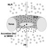 |
Fig. 1 Sketch of a quasar (based on Urry & Padovani 1995; Beckmann & Shrader 2012a): the super-massive black hole (SMBH), accretion disk, broad line region (BLR), narrow line region (NLR), jets, and the torus are shown. |
Quasars are Type 1 active galactic nuclei (AGNs), characterized by broad emission lines (BELs) with line widths of several tens of Angstroms in the quasar rest frame. Figure 1 shows their typical spatial structure schematically. Quasars contain super-massive black holes with masses of 106 to 1010M⊙ that are surrounded by an accretion disk. Using the relation between black hole mass and accretion disk size by Morgan et al. (2010), the accretion disks are typically smaller than 0.01 pc. The gravitational infall of gas and dust on this accretion disk produces the continuum emission of quasars. The surrounding broad emission line region (BLR) is smaller than or equal to ~1 pc and consists of clouds excited by accretion disk radiation. Cloud velocities larger than 500 km/s cause the BELs in this region. Because of high gas densities in the BLR, only permitted and semi-permitted broad emission lines occur. Farther out, there is a narrow line region (NLR) with cloud velocities about ten times smaller. The relation between the radius R and velocity v is R ~ v-2 (e.g., Peterson & Horne 2004). Hence, the size of the NLR is about 100 pc. Farther out, an expanded dusty torus surrounds the NLR region in quasars. The surface brightness of quasar host galaxies sharply decreases with redshift and hence the host galaxy is only visible for small redshifts (e.g., Disney et al. 1995; Bahcall et al. 1995; Kotilainen et al. 2009). Peterson (1997), Kembhavi & Narlikar (1999), and Beckmann & Shrader (2012b) describe the different quasar regions and unified models of AGNs in a general manner.
 |
Fig. 2 Rest-frame composite quasar spectrum after Vanden Berk et al. (2001). Gaia’s low-resolution (light region) and high-resolution (dark region) spectral ranges are indicated. The panel shows prominent broad emission lines Hα, Hβ, MgII, CIII], CIV, and Lyα. |
Quasar spectra typically have a very blue continuum and a number of broad emission lines. The spectra vary a lot from quasar to quasar, their typical features can be best seen in composite quasar spectra, like that of Vanden Berk et al. (2001), in Fig. 2. It considers about 2200 quasars from the Sloan Digital Sky Survey (SDSS) with r′ ≲ 19 for z ≲ 2.5 and r′ ≲ 20 for higher redshifts. Throughout this paper we use this composite quasar spectrum by Vanden Berk et al. (2001) as a template (from now on denoted as Vanden Berk et al. 2001), covering a rest-frame wavelength range between 800 Å and 8555 Å. Figure 2 shows the VB2001 spectrum together with the low-resolution (light blue area, 3300 Å−10 500 Å) and high-resolution (dark blue area, 8470 Å−8710 Å) wavelength regions of Gaia. In the plot we labeled the significant broad emission lines Hα, Hβ, MgII, CIII], CIV, and Lyα, which play an important role in our study.
In this paper, we use three different broadband denominations from three photometric systems (Gaia: G, Sloan: r′, Johnson: V) to indicate quasar magnitudes. In order to transform quasar brightnesses between G and r′ or V, we use magnitude correlations for SDSS quasars from Jester et al. (2005) and photometric relationships between Gaia photometry and existing photometric systems from Jordi (2013)3. In order to infer rough correlations between two magnitudes, we plotted DR7 quasars and applied a linear regression for different redshifts. We determine  The corresponding residual standard errors are 0.11 mag for both equations.
In order to achieve Gaia’s high positional accuracy, a quasar-based celestial reference frame is very important. For this, one requires about 10 000 bright quasars that are well distributed over the sky (Andrei et al. 2012; Mignard 2002). To identify quasars among other celestial objects, different approaches can be considered. First, the fraction of quasars is much higher at large Galactic latitudes because of stellar crowding in the Galactic plane. Second, quasars have characteristic blue spectra and they are variable, but especially for low equivalent width quasars at the faint end (low S/N) the spectral shapes are not unique, e.g., white dwarfs, F stars, and red dwarfs have similar colors to quasars at redshifts z< 0.5, z ~ 2.5, and z> 3, respectively (Claeskens et al. 2006). If one combines the various approaches with the absence of proper motion and parallax, it will be feasible to distinguish quasars from stellar objects (Mignard 2012). About one third of all Gaia quasars will be known AGNs; however, most will be new discoveries.
1.3. Quasar variability
In this paper, we present a potential quasar variability study with Gaia. Different continuum variability scenarios are discussed in the literature. Most likely a variable accretion rate or instabilities of the accretion disk are responsible for the spectral changes; for some objects, gravitational microlensing, supernova bursts, or jet instabilities are also possible explanations (e.g., Andrei et al. 2009; Popović et al. 2012). Furthermore, a hot corona above the SMBH produces X-ray photons. Reprocessing of these X-ray photons into UV-optical continuum radiation by the accretion disk could induce variability of short or medium timescale (Collin-Souffrin 1991; George & Fabian 1991; Gil-Merino et al. 2012).
If a quasar is variable, one can use this information to probe accretion physics and to calculate the BLR size and the mass of the black hole. This method is known as reverberation mapping, described in detail in, e.g., Peterson (1993) or Chelouche & Daniel (2012). The radiation (and variability) produced in the accretion disk needs a mean time τ to arrive at the BLR clouds. If one can determine this time lag, the BLR size is RBLR ≈ c·τ, where c is the speed of light. Together with the knowledge of the FWHM (full width at half maximum) of BELs, one can estimate the mass of the black hole (Peterson et al. 2004; Chelouche et al. 2012) by 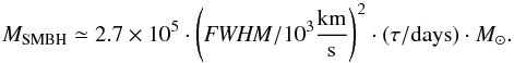 (3)Various SDSS quasar variability studies (e.g., Vanden Berk et al. 2004; Meusinger et al. 2011) have found that variability amplitudes decrease with wavelength and luminosity. In contrast, the time lag between continuum and BEL variability increases with wavelength. Furthermore, there is an anti-correlation between the equivalent widths of BELs (first discovered in the CIV line) and the luminosity of the nearby continuum, which is known as the Baldwin effect (Baldwin 1977). MacLeod et al. (2012) show that the optical continuum variability of their large SDSS quasar sample has timescales τ between 5 and 2000 days in the quasar rest frame.
Our paper is structured as follows: in Sect. 2, we analyze the spectrometric, photometric, and astrometric possibilities for quasar investigations with Gaia. In Sect. 3, we study quasars from the Sloan Digital Sky Survey (SDSS) with BELs in the spectral range of Gaia’s RVS in order to select a list of good candidates for a future variability analysis. Finally, we summarize the results and give an outlook in Sect. 4.
2. Quasar research with Gaia
In this section, we analyze the Gaia low- and high-resolution spectra of quasars, their signal-to-noise ratios (S/N) and the future opportunities to investigate the expected 500 000 Gaia quasars. For completeness, we summarize the literature of astrometric investigations of quasars with Gaia as well.
2.1. Simulating Gaia’s low-resolution spectra of quasars
In order to simulate low-resolution quasar spectra for Gaia, we convolved the VB2001 composite quasar spectrum with a Gaussian kernel. Additionally, in order to obtain realistic spectra, one has to consider the photon response curve of the Gaia CCDs, the spectral dispersion, and the number of data bins. We applied the photon response curve by Jordi et al. (2010) and included the spectral dispersions of the Blue and Red Photometers (BP and RP), which strongly depend on the wavelengths. The dispersion increases from 30 Å/pixel (at 3300 Å) to 270 Å/pixel (at 6800 Å) for the Blue Photometer, and 70 to 150 Å/pixel (at 6400 Å to 10 500 Å) for the Red Photometer. The line widths vary from 1.3 pixel (at 3300 Å) to 1.9 pixel (at 6800 Å) for BP, and 3.5 pixel (at 6400 Å) to 4.1 pixel (at 10 500 Å) for RP (de Bruijne 2012). Furthermore, Gaia’s low-resolution spectrum is subdivided into 75 data bins (Gaia term: “samples”), 37 for the blue area and 38 for the red area (Brown 2006). These samples are sets of pixels binned in the across-scan direction (Jordi et al. 2010).
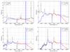 |
Fig. 3 Composite quasar spectra (Vanden Berk et al. 2001), convolved with Gaia’s low-resolution of the Blue and Red Photometers (BP and RP), for the magnitude G = 18 and redshifts z = 0.5, 1.5, 2.5, and 3.5. We plotted the resulting redshifted quasar spectra (black), BP low-resolution (blue), and RP low-resolution (red) spectra for the Gaia wavelength range considering Poisson noise and the photon response curve by Jordi et al. (2010). The blue shaded area indicates the spectral region of the RVS (8470−8710 Å). There are about 37 data bins (Gaia: “samples”) for the blue photometer and 38 samples for the red photometer resulting in example spectra represented by blue and red bars. We applied a typical exposure time for five single field-of-view passages (5 × 4.42 s) in order to calculate the number of photons. |
For a further analysis of Gaia’s quasar low-resolution spectra it is important to consider the S/N in our simulation. In order to analyze the S/N contributions to the low-resolution spectra, we studied Carrasco et al. (2006), who calculated the S/N per sample for different stellar types and magnitudes. The authors included effects like the sky background contribution, the total detection noise per sample, and calibration errors. The last effect has the strongest impact, the other contributions are negligible. Because of the multiplicity of spectral changes in redshifts and line widths, we studied the S/N for quasars from a stellar S/N diagram in Carrasco et al. (2006). As mentioned above, F stars have similar signatures to quasars at a redshift of about z ≈ 2.5 and so we compared the S/N graphs of F stars for different magnitudes (V = 10, 13, 16 mag) and calibration errors (σcal = 10, 40 mmag). From this analysis it follows that the calibration errors influence only bright objects (V ≲ 16 mag), samples with low S/N remain almost unchanged. Scaling the S/N to fainter objects, we conclude that the main noise contribution for quasar spectra is Poisson noise from the source (Bailer-Jones et al. 2008). From this, we can estimate that the S/N is proportional to the square root of the source flux. Hence, objects that are three magnitudes fainter have S/N that are approximately four times smaller. To determine the Poisson noise for all low-resolution quasar spectra at different magnitudes and redshifts, we scaled the composite spectrum to a SDSS quasar spectrum with these features. Furthermore, we converted the flux from erg/s/Å/cm2 into photons/Å considering an aperture of 1.45 m × 0.5 m and an exposure time (single CCD integration) of 4.42 s. As a result of several subsequent passages on the CCDs we increased the exposure time by a factor of five (five individual exposures).
2.2. Quasar low-resolution spectra for different magnitudes and redshifts
We use our analysis to plot quasar low-resolution spectra for different redshifts and magnitudes. First, we present convolved realistic Gaia spectra of quasars (blue and red) for redshifts z = 0.5, 1.5, 2.5, and 3.5 and magnitude G = 18 mag in Fig. 3. The redshifted input spectrum (VB2001) is shown as a black line. Depending on the redshift, different BELs like Lyα, CIV, CIII], MgII, Hβ, and Hα will fall in the two photometric ranges. At these four redshifts and magnitude G = 18 mag, there are enough BELs detectable to determine the quasar redshift. Bright quasars with large equivalent widths (like in the VB2001 template spectrum) would allow us to identify the object as a quasar from the low-resolution spectra alone. For a more precise prediction, we now analyze the low-resolution quasar spectra at magnitudes G = 16,18,19,20 mag and study the detectability of broad emission lines for redshifts between 0 <z< 5.
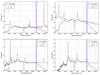 |
Fig. 4 Same as Fig. 3 for magnitude G = 20 and after 72 co-added observations (at the end of the mission). The redshift determination is feasible for most of the Gaia quasars until the magnitude limit of G = 20 mag. |
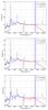 |
Fig. 5 Low-resolution spectra of VB2001 at redshift z = 2.5 for magnitudes G = 16,18,20 mag. We used the same data treated in the same way as in Fig. 3. The parts show the trend of increasing photon noise with fainter magnitude after a typical set of five observations. |
Depending on the quasar redshift, different broad emission lines are visible in Gaia’s BP or RP spectra. In order to determine reliable quasar redshifts, at least two BELs should be detectable between 3300 Å and 10 500 Å. Claeskens et al. (2006) analyzed the different redshift intervals in detail considering Gaia’s originally planed photometric system with 5 broadband and 14 medium-band filters. The authors mentioned that it should be easy to estimate the redshift because of its influence on the apparent wavelengths of strong BELs. However, Gaia’s photometric system was changed later (Jordi & Carrasco 2007), and so we studied redshift intervals for the photometric system that was in use at that time (BP and RP). We used simulated co-added spectra after five years of observations (72 measurements of two combined fields of view). Figure 4 shows the same composite quasar spectra as Fig. 3, but at G = 20 mag and at the end of the mission. Shifting the composite quasar spectrum between 0 <z< 5 at magnitude G = 20 mag, we always detected at least two BELs in the low-resolution spectra, but for some redshift ranges it will be more difficult to infer the redshift. At small redshifts (z ≲ 0.4) the Hα line is dominant and clearly detectable. The redshift interval 0.4 ≲ z ≲ 1.2 is the most difficult one; it shows several BELs (two out of the lines CIII], MgII, Hβ), but no prominent features, especially around z ≈ 1. This area will be very sensitive to noise, but if these objects are identified as quasars, a redshift determination is possible. Between 1.2 ≲ z ≲ 1.7, two lines out of CIV, CIII], and MgII are prominent. Furthermore, in the redshift interval 1.7 ≲ z ≲ 2.3 the CIV-line is dominant and Lyα, CIII], and MgII are in the BP/RP. The best region to determine the redshift is the range z ≳ 2.3, where the Lyα line dominates the spectra.
Some quasar spectra could be very different from the composite spectrum, especially for low equivalent width quasars, but for more quantitative studies, analyzing techniques like artificial neural networks or spectral principal component analysis have to be used, which was done in Claeskens et al. (2006) for the originally planed photometric system. The redshift errors vary with redshift and magnitude; they are in general smaller than Δz = 0.1, even at the faint end (Delchambre 2014).
In order to indicate the trend of noise with magnitude, we studied quasar spectra at a set of redshifts for different magnitudes. Additionally, we produced spectra with identical redshift and magnitude several times showing the possible variations in the individual samples. Figure 5 presents three quasar spectra with Gaia at a fixed redshift of z = 2.5 for the magnitudes G = 16,18, and 20 mag. In this example, the lines Lyα and CIV are detectable for all magnitudes. However, at G = 20 mag the noise level causes strong variations within the samples. Considering a series of these plots at identical redshift and magnitude, the photon noise allows quasar variability studies for all objects only down to G ≈ 18 mag.
2.3. Studying quasar variability from low-resolution spectra
Many quasars show strong variations in their spectra with time. In this section, we study the prospects of measuring the variability caused by different scenarios in quasar spectra with Gaia. Apart from continuum or broad line variability, we can also distinguish between short-term (intraday to days) and long-term (weeks to years) variations. In principle, Gaia’s scanning law allows us to follow up intraday (short-term) variability. However, only very bright quasars with large S/N and objects with high observational cadence, only achievable with many intraday measurements, are suitable for this variability scenario. For faint objects (G ≳ 18 mag), a combination of subsequent passages is necessary for a sufficiently high S/N. The precise magnitude limit for intraday variability studies depends on the quasar redshift and the kind of analyzed variations (BEL, BAL, or continuum changes). In contrast, long-term variations in quasar spectra are easy to observe, especially when they range from two months to a few years.
A small subsample of quasars will have much more than the typical 72 observations (e.g., at ecliptic latitudes around ± 45Å) within Gaia’s expected lifetime of five years. Many of these quasars will get additional measurements within a few days, but there are also objects with extra observations outside the intraday mode. These quasars are suitable for a large reverberation mapping campaign, so that the broad line region (BLR) structure can be investigated from the time lag. Another possibility for studying BELs is to measure their equivalent widths as a function of time. Since the equivalent widths of emission or absorption lines are independent of the resolution of the spectrograph, one can determine BEL equivalent widths from Gaia’s low-resolution spectra. Hence, it is possible to study the Baldwin effect for different broad emission lines. The FWHM, which is required for the determination of the black hole mass, depends on the resolution of the spectrograph. For both, the Blue and Red Photometer, one can only estimate the FWHM at their short wavelength range with higher resolution and in case of very large line width of several 1000 km s-1.
In order to investigate the continuum variability of Gaia quasars, we convolved 18 variable SDSS quasar spectra treated in the same way as the VB2001 quasar spectrum. The 18 quasars have SDSS r′ ≤ 17.6 mag, at least two available spectra in the SDSS bulk search tool, redshifts between 0.3 <z< 3.5, and they show clear continuum variations, like slope changes or flux jumps. Gaia’s low-resolution spectra make it possible to detect all of those continuum changes visible in the 18 example SDSS quasar spectra. We infer from the 18 SDSS quasar low-resolution spectra that one can in all cases analyze strong continuum flux changes, (fhigh(λ) − flow(λ)) /fhigh(λ) ~ 5%, and continuum slope changes for Gaia quasars with a magnitude of G< 18 mag. Depending on the quasar magnitude and the corresponding S/N, one might also be able to detect smaller flux changes for a few hundred objects. Figure 6 presents one example quasar from our sample of 18 objects. For this quasar (SDSS 154757.71+060626.6), we show the two available spectra from 2004 (red) and 2011 (black). The selected object has a redshift of z = 2.03 and a magnitude of r′ = 17.5 mag and it is a suitable example because of its strong variability. The bottom diagram of Fig. 6 shows the two spectra convolved with the low-resolution spectrometer of Gaia. For this convolution, we considered a sequence of five passages and Poisson noise. As can be seen, Gaia can easily detect such changes in continuum and equivalent widths.
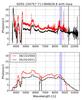 |
Fig. 6 Upper panel: spectra of the variable quasar SDSS 154757.71+060626.6 (Scaringi et al. 2009) in May 25, 2011 (black), and in October 6, 2004 (red). Bottom panel: same quasar spectra convolved with Gaia’s low-resolution instrument including noise and a sequence of five single-field-of-view observations. Gaia can easily detect such strong variability. |
Watson et al. (2011) have another idea, realized with a large reverberation mapping project. They describe a method of using an AGN as a cosmological distance measure. In this approach, the BLR size is related to the AGN luminosity and one can use this relation to calculate the luminosity-distance to the AGN. The method would allow reliable distance estimations up to z ~ 4 and potentially a test of dark energy and alternative gravity theories. Czerny & Hryniewicz (2011) explain the relation between the BLR size and the AGN monochromatic flux theoretically. In general, reverberation mapping campaigns have a high cadence (every few days) of observations in order to determine the time lag between continuum and various lines. Gaia will measure the objects several times within one day and then again, for instance two months later. For such a study, quasars with large observed time lags τ′ and significantly more than the average number of observations are required. The observed time lag τ′ = τ(1 + z) increases for high redshifts and large BLR radii. These BLR radii rise for very luminous quasars and for lower ionization lines. However, time lag measurements of quasars are very difficult. This holds especially for quasars with high luminosities, as they have only weak continuum variations or large redshifts, causing faint quasar magnitudes (e.g., Kaspi et al. 2007). Nevertheless, Gaia should be able to infer time lags of several luminous or high redshifted quasars. Additional ground-based observations for preselected quasars would complement the measurements and could fill the temporal gaps. The success of such an observational program will depend on the mathematical method to infer the time lag, the measurement accuracy, and on the selected BEL (Czerny et al. 2013).
Among BEL reverberation mapping, continuum responses to continuum variations are also observed. In this scenario, a blackbody accretion disk, having a temperature-radius-relation of T ~ r−3/4, reprocesses the high energy radiation of the central source (Collier et al. 1999). The reprocessing causes a time lag that depends on the wavelength (τ ~ λ4/3). Because of the small size of the accretion disk, the time lag has a typical value of a few days at large wavelength (λ ≈ 8000 Å). One could use the measurement of these time lags to analyze the accretion disk structure and to infer cosmological parameters like the Hubble constant. Furthermore, Collier et al. (1999) suggest using this method to determine redshift-independent luminosity distances to AGNs. However, because of the expected small time lags, only bright quasars (large S/N, G ≲ 18 mag) with high observational cadence (in this case many intraday measurements) are necessary to determine the wavelength dependent time lags with Gaia or complementary telescopes.
2.4. Gaia’s high-resolution spectra with the RVS
The Radial Velocity Spectrograph (RVS) of Gaia produces high-resolution spectra (R ~ 11 500) in the range 8470−8710 Å for objects brighter than GRVS = 17 mag. In this section we explain possible applications of the RVS for quasars considering the expected S/N for the faintest objects.
For certain quasar redshift ranges, emission or absorption lines fall into the narrow range (Δλ = 240 Å) of the Gaia RVS. In these cases, one can in principal analyze line profile and variability from the resulting high-resolution spectra. Analyzing the broad emission line shape with the RVS, one receives detailed information on the BLR of quasars. This is important because of the small size of the BLR, which is not spatially resolvable with current telescopes or Gaia. The line profile depends on, among other factors, different potential cloud velocities, the BLR geometry, obscuration effects, and superimposed emission lines from different quasar regions (Kollatschny & Zetzl 2013). Rotational motions of the line emitting clouds due to the Doppler effect produce Gaussian line profiles (e.g., Peterson & Wandel 1999), and outflowing gas can cause Logarithmic profiles (e.g., Blumenthal & Mathews 1975). Furthermore, turbulent motions in the outer accretion disk can explain Lorentzian line profiles (Goad et al. 2012). The ratio of this turbulent motion and the rotational velocity allows to investigate the thickness of the accretion disk (Kollatschny & Zetzl 2013). In the end, the measured line shape depends on various velocity components.
The S/N of lines in the RVS is an important quantity with which we can investigate the quasar variability in this wavelength interval. In order to infer the S/N as a function of the quasar brightness, we used a diagram of the S/N per sample of single CCDs as a function of the magnitude GRVS, which is only available for stars on the Gaia web page4. The RVS spectra contain about 1000 samples s between 8470 Å and 8710 Å. Its S/N per sample is relatively low, but we achieved sufficiently high S/N by rebinning the samples that cover the broad line. In particular we estimated the S/N in the FWHM of the lines Hα, Hβ, MgII, CIII], and CIV. Then we counted the number of samples in the FWHM of individual lines in the VB2001 composite quasar spectrum. In this calculation, we considered the redshift at which each individual line falls in the RVS. We took the FWHM values at redshift z = 0 from VB2001 and applied the relation FWHM(z) = (1 + z)·FWHM(z = 0). Furthermore, using the magnitude transformation equation mx = −2.5log (fx/fVega), we calculated the expected magnitude in the line width (mFWHM,line). To scale the composite quasar spectrum, we used individual SDSS spectra at characteristic redshift (BEL in the RVS) and several magnitude values between 14 ≲ GRVS ≲ 17. The resulting magnitude conversion for Hα is estimated to  (4)For the other lines this magnitude difference amounts to 0.36 mag (Hβ), 0.35 mag (MgII), 0.04 mag (CIII]), and 0.09 mag (CIV). Next we determined the S/N in the FWHM for each individual line by
  (5)The S/N is scaled by
  as a result of the information from three CCDs for every single measurement. Figure 7 shows our resulting FWHM-S/N of every emission line as a function of the magnitude GRVS. The five different emission lines have slightly different values of S/N. At the faint end (GRVS ≈ 17), where most of the quasars are located, the S/N in the FWHM is only about five to seven. The Hβ line, which exhibits the smallest equivalent width, has the smallest S/N value. In order to confirm our estimate, we calculated the S/N in the FWHM in a second way. In this approach, we determined the S/N in every sample for all BELs falling in the RVS. From this, we recomputed the S/N in the FWHM for different magnitudes with the equation
 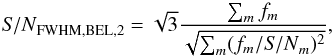 (6)where index m is the sample number, fm the sample flux, and S/Nm the sample S/N. Table 1 lists selected results for this second S/N approach for various values of GRVS. If we compare the values in Fig. 7 and Table 1, we find similar results for the S/N values. Hence we conclude that our results from the first S/N approach, presented in Fig. 7, are a good estimation of the S/N in the BEL FWHM.
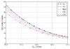 |
Fig. 7 Estimated S/N against GRVS between 15 and 17 mag for Hα, Hβ, MgII, CIII], and CIV in Gaia’s RVS. For the limiting magnitude of GRVS ≈ 17, the S/N in the BEL is only about five to seven. |
We conclude that one will learn more about the dynamics and spatial structure of the broad emission line region, at least for several hundred objects, by studying the broad emission line shapes with Gaia’s RVS. Furthermore, the combination of low- and high-resolution spectra will increase the potential information for quasar investigations. For example, one could use the RVS to measure the FWHM of a broad emission line; but to identify this line, one has to derive the quasar redshift from Gaia’s BP/RP low-resolution spectra. Additionally, objects with high observational cadence or large time lags allow us to determine the time lag between continuum and BEL radiation. Hence, one can calculate the black hole mass using the FWHM from the RVS and the time lag from BP/RP observations. For the detection of broad emission line FWHM, one has to consider turbulent motions, otherwise one would overestimate black hole masses (Kollatschny & Zetzl 2013). If we determine the BEL response to continuum variations, we could distinguish intrinsic BEL variability from continuum variability with the help of the RVS. However, the S/N of quasar narrow absorption lines and broad absorption lines in the RVS is too low to analyze their nature.
Signal-to-noise ratios in the FWHM of quasar broad emission lines for different values of GRVS.
2.5. Quasars with broad emission lines in the Gaia high-resolution spectrometer (RVS)
Because of the small RVS wavelength range (Δλ = 8710 Å−8470 Å = 240 Å) and its limiting magnitude of GRVS = 17 mag, only a small subset of Gaia quasars are in redshift regions where BELs would fall into the RVS range. In total, the simulated Gaia catalog by Robin et al. (2012) contains 106 quasars, of which 5200 objects are bright enough to be detected in the RVS. From these bright quasars, 579 objects have broad lines in the RVS wavelength area. The quasars in this simulated Gaia catalog were produced mainly with similar statistical properties as SDSS (e.g., colors, apparent brightness, redshifts), but extrapolated to G = 20.5 mag (Slezak & Mignard 2007). Additionally, Robin et al. (2012) considered a sky coverage for Gaia quasars of about only 2/3 because of crowding in the Galactic plane.
We searched through all SDSS quasars for BELs detectable in Gaia’s RVS considering these redshifts and magnitudes. In order to get the correct magnitude limit, we had to convert a SDSS magnitude (z′) to Gaia’s magnitude GRVS. The magnitude difference is quite different for individual quasars, but for our selected sample of objects z′ was typically between 0.5 and 1.0 mag fainter than the corresponding GRVS. Hence, we chose the magnitude limit z′ = 17.5 mag (r′ = 17.6 mag) for SDSS objects which have broad emission lines in the wavelength range of Gaia’s RVS. Since we noticed several incorrect quasar identifications or erroneous redshifts in the SDSS quasar catalog (Schneider et al. 2010), we checked all 608 bright candidates with BELs in the RVS individually using the SDSS bulk spectra search tool. Considering the magnitude limit and redshift intervals for objects in the SDSS survey, which has a sky coverage of only ~1/3, we identified 535 quasars fulfilling our criteria. Table 2 shows the described wavelength ranges for Hα, Hβ, MgII, CIII], and CIV, where at least one wing (~50% of the BEL) is located in the RVS interval. Furthermore, we listed the number of expected quasars from the simulated Gaia catalog (Robin et al. 2012) and the SDSS objects in the different wavelength ranges. As expected, because of the large number of bright quasars in this redshift range, most of the simulated Gaia or SDSS quasars with a line in the RVS range have the broad Hα line in this interval. Figure 8 presents the expected number of quasars with potential RVS data in a histogram for redshift bins of Δz = 0.2 (red). In this histogram, the expected quasars from Robin et al. (2012) with BELs in the RVS are shown in black, the redshift bin widths are given in Table 2.
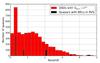 |
Fig. 8 Redshift distribution of ~5200 simulated Gaia quasars from Robin et al. (2012) brighter than GRVS = 17 mag in redshift bins of 0.2 (red). The fraction of these quasars that also have a broad emission line in the RVS (579 objects) are shown in black. Their smaller bin widths represent the redshift range when at least one BEL wing falls in the RVS pass band (see Table 2). |
Redshift ranges for which specific quasar emission lines would fall into the Gaia RVS.
2.6. Astrometric quasar analysis with Gaia
In this section, we summarize potential astrometric investigations of quasars from the literature. Furthermore, we give an outlook on whether it is possible to detect potential astrometric shifts with the Gaia satellite.
Taris et al. (2011) describe an interaction between flux variability and photocenter changes in quasars. Based on this investigation, Popović et al. (2012) simulate the variability of the photocenter related to variations in the accretion disk and the dust torus of quasars. They estimate that accretion disk perturbations of low-redshift AGNs with huge black hole mass (≳ 109M⊙) may induce photocenter shifts of a few milliarcseconds. In addition, torus related photocenter offsets, which result from illuminations when dust covers the central region, could be as large as several milliarcseconds. In principle these effects would be observable with Gaia. Furthermore, Popović et al. (2012) emphasize that Gaia’s quasar sample for construction of the reference frame should not include such objects with photocenter variability.
Shen (2012) explores the opportunity of astrometric reverberation mapping. In the case of a BLR with non-spherically symmetric spatial structure or velocity distribution, photocenter variations with time are induced by different BLR arrival times of continuum variations. In addition to common reverberation mapping, astrometric reverberation mapping would offer independent constraints on geometry and kinematic configuration of BLRs like inclination or rotation angles. For typical quasar luminosities and a redshift of z ≈ 0.5, the author determines expected photocenter offsets of some tens of microarcseconds, or slightly larger for dust tori astrometric reverberation mapping. Hence Gaia’s astrometric accuracy for a single observation of quasars would not be sufficient to measure astrometric reverberation mapping of their BLR. It is also unlikely to measure the event for dust tori of quasars.
Another application of very accurate astrometry with quasars is astrometric microlensing. This effect causes a small shifts of quasar positions, which are gravitationally lensed by foreground galaxies. Astrometric microlensing can cause center-of-light (centroid) displacements (Lewis & Ibata 1998). This centroid is the weighted sum of all unresolved microimages produced by microlensing, and it can move as a result of the creation of a bright pair of microimages during a caustic crossing. The photocenter shift in quasars by astrometric microlensing of stellar mass objects in the lensing galaxy could be on the order of tens of microarcseconds and has a timescale of months to years (Treyer & Wambsganss 2004). Even if Gaia might not be able to measure the astrometric microlensing effect in quasar sources by single stars, microlensing induced by small mass stellar clusters in the lensing galaxy could cause centroid shifts of several milliarcseconds (Popović & Simić 2013), which would be detectable with Gaia.
3. SDSS quasars with Gaia
In this section, we present a list of known variable SDSS quasars which will have BELs in Gaia’s RVS range. They are interesting candidates for line variability investigations, which are caused by changes in the BLR itself, or variations related to continuum responses. SDSS spectra in general have a resolution λ/ Δλ of about 2000 and a wavelength range slightly smaller than Gaia’s low-resolution spectra.
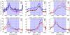 |
Fig. 9 Six variable SDSS quasars which are listed in Table 3 (1 to 6) considering the available SDSS spectra (Schneider et al. 2010). All candidates are brighter than GRVS = 17 mag and have BELs in Gaia’s RVS. We indicate the wavelength range of the high-resolution spectrum in blue. Gaia’s high-resolution spectra would allow the study of their presented (intrinsic) line variability. |
Interesting quasars with BELs in the Radial Velocity Spectrograph.
We searched for quasars with at least two available spectra in the SDSS data release 7 database (Schneider et al. 2010) and studied their variability features. From this, we obtained a candidate list, whose spectra we examined for incorrect flux changes. To eliminate possible flux calibration errors, we analyzed stellar spectra with same Plate and Julian Date information. Additionally, in the case of existing narrow absorption lines, their normalization was tested, too. Some objects had suspicious continuum flux changes, but if they showed interesting spectral features and their narrow lines were normalized correctly, they were kept in our list. The S/N aspect is considered for most of the preselected candidates as well. In this process, we found six interesting SDSS quasars with either strong BEL variability or rapid continuum variability of weeks or months that should result in a BEL variability as well. Furthermore, we identified a bright multiply lensed quasar and a physical binary quasar in the CASTLE Survey (Kochanek et al. 2013) that have a BEL in the RVS range5. We could not analyze the variability of these two quasars because several spectra were missing. Table 3 lists these two sets of interesting quasar candidates together with information on magnitudes, epochs of spectra, and the affected BEL.
In Fig. 9 we present the spectra of those six SDSS quasars in the wavelength region of Gaia’s high-resolution spectra (blue). We found that candidates 1 and 2 displayed strong continuum shifts within weeks or months and that candidate 3 shows strong BEL variations, but only small continuum changes. Candidates 4 and 6 are variable in continuum and BEL. We recognized that the continuum flux for λ< 6000 Å of candidate 5 is erroneous (the jump in the blue part of the spectrum is also visible in parallel stellar spectra), but its BEL variability seems real. Candidates 1 and 5 have very low values of S/N and hence they will have very noisy Gaia spectra. Spectral analyses with Gaia of these six SDSS quasars with interesting variability signatures, the multiply lensed quasar, and the binary quasar offer very promising BLR structure investigations, as described in Sect. 2.4.
4. Summary
We analyzed the opportunities that the low- and high-resolution Gaia spectrometers offer with respect to quasars. We generated and analyzed low-resolution spectra (BP/RP) based on the composite quasar spectrum from VB2001 considering different redshifts and the Poisson noise for magnitudes G = 16,18, and 20 mag. According to these realistic low-resolution spectra, we concluded that redshift determinations and equivalent width (Baldwin effect) detections are possible for most quasars brighter than G = 20 mag; continuum variability studies should be performed at least for quasars brighter than G = 18 mag. Furthermore, time lags between continuum and broad line region can be inferred from Gaia’s Blue and Red Photometer for bright objects with high observational cadence, e.g., in the proximity of ± 45° in ecliptic latitudes. For the typical number of measurements, only large time lags (on the order of several months) can be detected. The time lags increase for high redshifts (time dilation), large quasar luminosities, or the selection of low-ionization lines. For a small number of bright quasars (G ≲ 18 mag) with high observational cadence, achieved with intraday measurements, it could be also possible to investigate short-term variations in the continuum with Gaia.
All objects with GRVS< 17 mag in the RVS will have high-resolution spectra in the wavelength range between 8470 Å and 8710 Å. We identified 579 quasars in the simulated Gaia catalog of Robin et al. (2012), based on statistical properties of mainly SDSS quasars, which are bright enough and have BELs (Hα, Hβ, MgII, CIII], or CIV) in the RVS redshift range. For those quasars, out of the ~600 objects, with GRVS ≈ 17 mag, the FWHM signal-to-noise ratio of BELs in the RVS is very low (~ 5 to 7), which means that not all ~600 objects are suitable for a successful variability study. This also depends on the achieved real magnitude limit (GRVS) of Gaia. For the remaining objects (GRVS ≲ 16.5 mag), the RVS enables an intrinsic line variability analysis (line profiles and their variabilities). A combination of low- and high-resolution spectra of these roughly 600 Gaia quasars will enhance the BEL study. An example is the calculation of the FWHM of a broad emission line with the RVS. Additionally, one can identify this line and determine the time lag between line and continuum with the Blue or Red Photometer. The combination of the data can be used to infer the mass of the black hole.
Our variability investigation of known bright SDSS quasars with BELs in the RVS resulted in six interesting candidates. Furthermore, a multiply lensed quasar (HE2149-2745) and a physical binary quasar (LBQS1429-008) will get high-resolution spectra of their broad lines in Gaia’s RVS wavelength range. These interesting quasar candidates should be observed in parallel with ground-based observations within Gaia’s expected lifetime of five years to study intrinsic line variabilities or line responses to continuum variations. Such analyses will improve our understanding of the spatial geometry and kinematics in the broad line region, and the interaction between BLR and accretion disk.
Acknowledgments
We wish to thank the members of the gravitational lensing group at ARI for helpful comments and discussions, and Ulrich Bastian and Coryn Bailer-Jones for information about the Gaia mission. We would like to particularly thank the anonymous referee for very constructive comments which helped to improve the manuscript significantly. J.W. acknowledges with great pleasure generous support received during his tenure as Schroedinger Visiting Professor 2013 at the Pauli Center for Theoretical Studies in Zurich (Switzerland) which is supported by the Swiss National Science Foundation (SNF), ETH Zurich, and the University of Zurich. Funding for SDSS-III has been provided by the Alfred P. Sloan Foundation, the Participating Institutions, the National Science Foundation, and the US Department of Energy Office of Science. The SDSS-III web site is http://www.sdss3.org/. SDSS-III is managed by the Astrophysical Research Consortium for the Participating Institutions of the SDSS-III Collaboration including the University of Arizona, the Brazilian Participation Group, Brookhaven National Laboratory, University of Cambridge, University of Florida, the French Participation Group, the German Participation Group, the Instituto de Astrofisica de Canarias, the Michigan State/Notre Dame/JINA Participation Group, Johns Hopkins University, Lawrence Berkeley National Laboratory, Max Planck Institute for Astrophysics, New Mexico State University, New York University, Ohio State University, Pennsylvania State University, University of Portsmouth, Princeton University, the Spanish Participation Group, University of Tokyo, University of Utah, Vanderbilt University, University of Virginia, University of Washington, and Yale University.
References
- Andrei, A. H., Souchay, J., Zacharias, N., et al. 2009, A&A, 505, 385 [NASA ADS] [CrossRef] [EDP Sciences] [MathSciNet] [Google Scholar]
- Andrei, A. H., Anton, S., Barache, C., et al. 2012, Mem. Soc. Astron. Ita., 83, 930 [Google Scholar]
- Bahcall, J. N., Kirhakos, S., & Schneider, D. P. 1995, ApJ, 450, 486 [NASA ADS] [CrossRef] [Google Scholar]
- Bailer-Jones, C. A. L., Smith, K. W., Tiede, C., et al. 2008, MNRAS, 391, 1838 [NASA ADS] [CrossRef] [Google Scholar]
- Baldwin, J. A. 1977, ApJ, 214, 679 [NASA ADS] [CrossRef] [Google Scholar]
- Beckmann, V., & Shrader, C. 2012a, in Proc. An INTEGRAL view of the high-energy sky (the first 10 years) – 9th INTEGRAL Workshop and celebration of the 10th anniversary of the launch (INTEGRAL 2012) [Google Scholar]
- Beckmann, V., & Shrader, C. R. 2012b, Active Galactic Nuclei (Wiley-VCH Verlag GmbH) [Google Scholar]
- Blumenthal, G. R., & Mathews, W. G. 1975, ApJ, 198, 517 [NASA ADS] [CrossRef] [Google Scholar]
- Brown, A. 2006, Simulating Prism Spectra for the EADS-Astrium Gaia Design, Internal Gaia Report: GAIA-CA-TN-LEI-AB-005-7, Tech. Rep. [Google Scholar]
- Carrasco, J. M., Jordi, C., Figueras, F., Anglada-Escudé, G., & Amores, E. B. 2006, GAIA-C5-TN-UB-JMC-001-2, Tech. Rep. [Google Scholar]
- Chelouche, D., & Daniel, E. 2012, ApJ, 747, 62 [NASA ADS] [CrossRef] [Google Scholar]
- Chelouche, D., Daniel, E., & Kaspi, S. 2012, ApJ, 750, L43 [NASA ADS] [CrossRef] [Google Scholar]
- Claeskens, J.-F., Smette, A., Vandenbulcke, L., & Surdej, J. 2006, MNRAS, 367, 879 [NASA ADS] [CrossRef] [Google Scholar]
- Collier, S., Horne, K., Wanders, I., et al. 1999, MNRAS, 302, L24 [NASA ADS] [CrossRef] [Google Scholar]
- Collin-Souffrin, S. 1991, A&A, 249, 344 [NASA ADS] [Google Scholar]
- Czerny, B., & Hryniewicz, K. 2011, A&A, 525, L8 [NASA ADS] [CrossRef] [EDP Sciences] [Google Scholar]
- Czerny, B., Hryniewicz, K., Maity, I., et al. 2013, A&A, 556, A97 [NASA ADS] [CrossRef] [EDP Sciences] [Google Scholar]
- de Bruijne, J. H. J. 2012, Ap&SS, 341, 31 [NASA ADS] [CrossRef] [Google Scholar]
- Delchambre, L. 2014, GWP-S-831 Software Test Report for Cycle 15, Gaia Report: GAIA-C8-TR-IAGL-LD-003-15, Tech. Rep. [Google Scholar]
- Disney, M. J., Boyce, P. J., Blades, J. C., et al. 1995, Nature, 376, 150 [NASA ADS] [CrossRef] [Google Scholar]
- Eyer, L., Holl, B., Pourbaix, D., et al. 2013, Central European Astrophysical Bulletin, 37, 115 [NASA ADS] [Google Scholar]
- Finet, F., Elyiv, A., & Surdej, J. 2012, Mem. Soc. Astron. Ital., 8, 83, 944 [Google Scholar]
- George, I. M., & Fabian, A. C. 1991, MNRAS, 249, 352 [NASA ADS] [CrossRef] [Google Scholar]
- Gil-Merino, R., Goicoechea, L. J., Shalyapin, V. N., & Braga, V. F. 2012, ApJ, 744, 47 [NASA ADS] [CrossRef] [Google Scholar]
- Goad, M. R., Korista, K. T., & Ruff, A. J. 2012, MNRAS, 426, 3086 [NASA ADS] [CrossRef] [Google Scholar]
- Hudec, R., et al. 2010, Adv. Astron., 2010, 7 [Google Scholar]
- Jester, S., Schneider, D. P., Richards, G. T., et al. 2005, AJ, 130, 873 [NASA ADS] [CrossRef] [Google Scholar]
- Jordi, C. 2013, Photometric relationships between Gaia photometry and existing photometric systems, Gaia Report: GAIA-C5-TN-UB-CJ-041-8, Tech. Rep. [Google Scholar]
- Jordi, C., & Carrasco, J. M. 2007, in The Future of Photometric, Spectrophotometric and Polarimetric Standardization, ed. C. Sterken, ASP Conf. Ser., 364, 215 [NASA ADS] [Google Scholar]
- Jordi, C., Gebran, M., Carrasco, J. M., et al. 2010, A&A, 523, A48 [NASA ADS] [CrossRef] [EDP Sciences] [Google Scholar]
- Kaspi, S., Brandt, W. N., Maoz, D., et al. 2007, ApJ, 659, 997 [NASA ADS] [CrossRef] [Google Scholar]
- Kembhavi, A. K., & Narlikar, J. V. 1999, Quasars and active galactic nuclei: an introduction (Cambridge University Press) [Google Scholar]
- Kochanek, C., Falco, E., Impey, C., et al. 2013, CASTLES Survey: Gravitational Lens Data Base, project homepage, Harvard-Smithsonian Center for Astrophysics, http://cfa-www.harvard.edu/glensdata/ (accessed on 1 December 2013) [Google Scholar]
- Kollatschny, W., & Zetzl, M. 2013, A&A, 549, A100 [NASA ADS] [CrossRef] [EDP Sciences] [Google Scholar]
- Kotilainen, J. K., Falomo, R., Decarli, R., et al. 2009, ApJ, 703, 1663 [NASA ADS] [CrossRef] [Google Scholar]
- Lewis, G. F., & Ibata, R. A. 1998, ApJ, 501, 478 [NASA ADS] [CrossRef] [Google Scholar]
- Lindegren, L. 2010, in IAU Symp. 261, eds. S. A. Klioner, P. K. Seidelmann, & M. H. Soffel, 296 [Google Scholar]
- MacLeod, C. L., Ivezić, v., Sesar, B., et al. 2012, ApJ, 753, 106 [NASA ADS] [CrossRef] [Google Scholar]
- Meusinger, H., Hinze, A., & de Hoon, A. 2011, A&A, 525, A37 [NASA ADS] [CrossRef] [EDP Sciences] [Google Scholar]
- Mignard, F. 2002, in eds. O. Bienayme & C. Turon, EAS Pub. Ser. 2, 327 [Google Scholar]
- Mignard, F. 2012, Mem. Soc. Astron. Italiana, 83, 918 [Google Scholar]
- Morgan, C. W., Kochanek, C. S., Morgan, N. D., & Falco, E. E. 2010, ApJ, 712, 1129 [NASA ADS] [CrossRef] [Google Scholar]
- Perryman, M. A. C., de Boer, K. S., Gilmore, G., et al. 2001, A&A, 369, 339 [NASA ADS] [CrossRef] [EDP Sciences] [Google Scholar]
- Peterson, B. M. 1993, PASP, 105, 247 [NASA ADS] [CrossRef] [Google Scholar]
- Peterson, B. M. 1997, An introduction to active galactic nuclei (Cambridge University Press) [Google Scholar]
- Peterson, B. M., & Horne, K. 2004, Astron. Nachr., 325, 248 [Google Scholar]
- Peterson, B. M., & Wandel, A. 1999, ApJ, 521, L95 [NASA ADS] [CrossRef] [Google Scholar]
- Peterson, B. M., Ferrarese, L., Gilbert, K. M., et al. 2004, ApJ, 613, 682 [NASA ADS] [CrossRef] [Google Scholar]
- Popović, L. V., & Simić, S. 2013, MNRAS, 432, 848 [NASA ADS] [CrossRef] [Google Scholar]
- Popović, L. V., Jovanović, P., Stalevski, M., et al. 2012, A&A, 538, A107 [NASA ADS] [CrossRef] [EDP Sciences] [Google Scholar]
- Robin, A. C., Luri, X., Reylé, C., et al. 2012, A&A, 543, A100 [NASA ADS] [CrossRef] [EDP Sciences] [Google Scholar]
- Scaringi, S., Cottis, C. E., Knigge, C., & Goad, M. R. 2009, MNRAS, 399, 2231 [NASA ADS] [CrossRef] [Google Scholar]
- Schneider, D. P., Richards, G. T., Hall, P. B., et al. 2010, VizieR Online Data Catalog: VII/260 [Google Scholar]
- Shen, Y. 2012, ApJ, 757, 152 [NASA ADS] [CrossRef] [Google Scholar]
- Slezak, E., & Mignard, F. 2007, A realistic QSO Catalogue for the Gaia Universe Model, Gaia-c2-tn-oca-es-001-1, Observatoire de la Côte d’Azur [Google Scholar]
- Taris, F., Souchay, J., Andrei, A. H., et al. 2011, A&A, 526, A25 [NASA ADS] [CrossRef] [EDP Sciences] [Google Scholar]
- Treyer, M., & Wambsganss, J. 2004, A&A, 416, 19 [NASA ADS] [CrossRef] [EDP Sciences] [Google Scholar]
- Urry, C. M., & Padovani, P. 1995, PASP, 107, 803 [NASA ADS] [CrossRef] [Google Scholar]
- Vanden Berk, D. E., Richards, G. T., Bauer, A., et al. 2001, AJ, 122, 549 (VB2001) [NASA ADS] [CrossRef] [Google Scholar]
- Vanden Berk, D. E., Wilhite, B. C., Kron, R. G., et al. 2004, ApJ, 601, 692 [NASA ADS] [CrossRef] [Google Scholar]
- Voss, H., Jordi, C., Fabricius, C., et al. 2013, in Highlights of Spanish Astrophysics VII, 738 [Google Scholar]
- Watson, D., Denney, K. D., Vestergaard, M., & Davis, T. M. 2011, ApJ, 740, L49 [NASA ADS] [CrossRef] [Google Scholar]
All Tables
Signal-to-noise ratios in the FWHM of quasar broad emission lines for different values of GRVS.
Redshift ranges for which specific quasar emission lines would fall into the Gaia RVS.
All Figures
|
Fig. 1 Sketch of a quasar (based on Urry & Padovani 1995; Beckmann & Shrader 2012a): the super-massive black hole (SMBH), accretion disk, broad line region (BLR), narrow line region (NLR), jets, and the torus are shown. |
| In the text | |
|
Fig. 2 Rest-frame composite quasar spectrum after Vanden Berk et al. (2001). Gaia’s low-resolution (light region) and high-resolution (dark region) spectral ranges are indicated. The panel shows prominent broad emission lines Hα, Hβ, MgII, CIII], CIV, and Lyα. |
| In the text | |
|
Fig. 3 Composite quasar spectra (Vanden Berk et al. 2001), convolved with Gaia’s low-resolution of the Blue and Red Photometers (BP and RP), for the magnitude G = 18 and redshifts z = 0.5, 1.5, 2.5, and 3.5. We plotted the resulting redshifted quasar spectra (black), BP low-resolution (blue), and RP low-resolution (red) spectra for the Gaia wavelength range considering Poisson noise and the photon response curve by Jordi et al. (2010). The blue shaded area indicates the spectral region of the RVS (8470−8710 Å). There are about 37 data bins (Gaia: “samples”) for the blue photometer and 38 samples for the red photometer resulting in example spectra represented by blue and red bars. We applied a typical exposure time for five single field-of-view passages (5 × 4.42 s) in order to calculate the number of photons. |
| In the text | |
|
Fig. 4 Same as Fig. 3 for magnitude G = 20 and after 72 co-added observations (at the end of the mission). The redshift determination is feasible for most of the Gaia quasars until the magnitude limit of G = 20 mag. |
| In the text | |
|
Fig. 5 Low-resolution spectra of VB2001 at redshift z = 2.5 for magnitudes G = 16,18,20 mag. We used the same data treated in the same way as in Fig. 3. The parts show the trend of increasing photon noise with fainter magnitude after a typical set of five observations. |
| In the text | |
|
Fig. 6 Upper panel: spectra of the variable quasar SDSS 154757.71+060626.6 (Scaringi et al. 2009) in May 25, 2011 (black), and in October 6, 2004 (red). Bottom panel: same quasar spectra convolved with Gaia’s low-resolution instrument including noise and a sequence of five single-field-of-view observations. Gaia can easily detect such strong variability. |
| In the text | |
|
Fig. 7 Estimated S/N against GRVS between 15 and 17 mag for Hα, Hβ, MgII, CIII], and CIV in Gaia’s RVS. For the limiting magnitude of GRVS ≈ 17, the S/N in the BEL is only about five to seven. |
| In the text | |
|
Fig. 8 Redshift distribution of ~5200 simulated Gaia quasars from Robin et al. (2012) brighter than GRVS = 17 mag in redshift bins of 0.2 (red). The fraction of these quasars that also have a broad emission line in the RVS (579 objects) are shown in black. Their smaller bin widths represent the redshift range when at least one BEL wing falls in the RVS pass band (see Table 2). |
| In the text | |
|
Fig. 9 Six variable SDSS quasars which are listed in Table 3 (1 to 6) considering the available SDSS spectra (Schneider et al. 2010). All candidates are brighter than GRVS = 17 mag and have BELs in Gaia’s RVS. We indicate the wavelength range of the high-resolution spectrum in blue. Gaia’s high-resolution spectra would allow the study of their presented (intrinsic) line variability. |
| In the text | |
Current usage metrics show cumulative count of Article Views (full-text article views including HTML views, PDF and ePub downloads, according to the available data) and Abstracts Views on Vision4Press platform.
Data correspond to usage on the plateform after 2015. The current usage metrics is available 48-96 hours after online publication and is updated daily on week days.
Initial download of the metrics may take a while.