| Issue |
A&A
Volume 573, January 2015
|
|
|---|---|---|
| Article Number | A75 | |
| Number of page(s) | 7 | |
| Section | Cosmology (including clusters of galaxies) | |
| DOI | https://doi.org/10.1051/0004-6361/201424586 | |
| Published online | 19 December 2014 | |
Extending the LX – T relation from clusters to groups
Impact of cool core nature, AGN feedback, and selection effects
Argelander-Institut für Astronomie,
Auf dem Hügel 71,
53121
Bonn,
Germany
e-mail:
This email address is being protected from spambots. You need JavaScript enabled to view it.
Received: 11 July 2014
Accepted: 17 October 2014
Abstract
Aims. We aim to investigate the bolometric LX − T relation for galaxy groups, and to study the impact of gas cooling, feedback from super-massive black holes, and the selection effects on it.
Methods. With a sample of 26 galaxy groups, we obtained the best-fit LX − T relation for five different cases depending on the intracluster medium (ICM) core properties and central active galactic nuclei (AGN) radio emission, and determined the slopes, normalisations, and intrinsic and statistical scatters for both temperature and luminosity. We undertook simulations to correct for selection effects (e.g. Malmquist bias) and compared the bias-corrected relations for groups and clusters.
Results. The slope of the bias-corrected LX − T relation is marginally steeper, but consistent with clusters (~3). Groups with a central cooling time of less than 1 Gyr (SCC groups) show indications of having the steepest slope and the highest normalisation. For the groups, the bias-corrected intrinsic scatter in LX is larger than the observed scatter for most cases, and this is reported here for the first time. We see indications that the groups with an extended central radio source (CRS) have a much steeper slope than those groups that have a CRS with only core emission. Additionally, we see indications that the more powerful radio AGN are preferentially located in non strong cool core (NSCC) groups rather than strong cool core (SCC) groups.
Key words: galaxies: clusters: intracluster medium / galaxies: groups: general / X-rays: galaxies: clusters
© ESO, 2014
1. Introduction
A naive starting point when defining groups of galaxies is to simply call them scaled down versions of galaxy clusters. This is not entirely out of context, as the distinction between “groups” and “clusters” is quite loose and no universal definition exists in the literature. However, groups and clusters have some notable differences, such as a lack of dominance of the intracluster medium (ICM) over the galactic component (e.g. Giodini et al. 2009). Moreover, because of the shallower gravitational potential of groups, one would expect processes like active galactic nuclei (AGN) heating and galactic winds to leave stronger imprints on the group ICM than in the cluster ICM. As a result of the shape of the cluster mass function (e.g. Tinker et al. 2008; Vikhlinin et al. 2009), most “clusters” are in fact groups of galaxies, and consequently, most galaxies in the local Universe are present in groups. The upcoming X-ray telescope eROSITA (Predehl et al. 2010) on the Spektrum-Roentgen-Gamma (SRG) mission promises to detect 105 clusters, most of which will be galaxy groups (Pillepich et al. 2012). Most of these systems would lack sufficient X-ray counts to be able to measure temperature and mass accurately (Borm et al. 2014), meaning an observable proxy, such as luminosity, or external constraints, such as weak lensing follow-up (Merloni et al. 2012), would have to be used to constrain these properties. In order to achieve this, the construction of robust, precise, and unbiased scaling relations using existing data gains paramount importance.
Scaling relations such as LX − Mtot, LX − T and Mtot − T have been well established for different samples of galaxy clusters (e.g. Allen et al. 2001; Reiprich & Böhringer 2002; Vikhlinin et al. 2006; see Giodini et al. 2013, for a review). The validity of cluster scaling relations on the group scale has led to conflicting viewpoints, with Ponman et al. (1996) suggesting variations for galaxy groups, and e.g. Sun et al. (2009) refuting any discrepancy between clusters and groups. Eckmiller et al. (2011) show that there is a good agreement between clusters and groups for most scaling relations, albeit with increased intrinsic scatter on the group regime, which is not totally unexpected due to the complicated baryonic physics at play in low-mass systems. Recent results by Lovisari et al. (2014), however, argue that while the observed scaling relations for galaxy groups are in agreement with those obtained for galaxy clusters, the scaling relation obtained after corrections for selection effects are consistent with a gradual steepening towards the low-mass regime.
The  relation is one of the most contentious scaling relations. Self-similarity predicts that the bolometric LX is proportional to T2 (e.g. Eke et al. 1998) for clusters, but observations constrain a much steeper slope (e.g. Arnaud & Evrard 1999). Moreover, as compared to other scaling relations, the intrinsic scatter is also much larger (e.g. Pratt et al. 2009). A major contribution to the scatter in the scaling relation is the cooling gas in the cores of clusters, as shown by e.g. O’Hara et al. (2006). Mittal et al. (2011) in particular demonstrate that excising the core regions reduce the scatter in the LX − T relation by 27%, additionally stating that cool cores cannot be the sole contributor to the scatter. They also speculate that while ICM cooling dominates the cluster regime, AGN feedback could have a greater effect on the scaling relation in groups, mainly due to the shallower gravitational potential of these systems.
This paper is the first systematic attempt to determine bolometric LX − T relations to account for both the presence/absence of a strong cool core and the presence/absence of a central radio loud AGN in galaxy groups. Additionally, we construct a bias corrected bolometric LX − T relation to objectively compare groups and clusters of galaxies for the first time. The overarching theme of this paper is to understand the impact of non-gravitational processes and the selection effects on the LX − T relation.
A ΛCDM cosmology with Ωm = 0.27, ΩΛ = 0.73 and h = 0.71 where H0 = 100 h km s-1/Mpc is assumed throughout the paper, unless stated otherwise. All errors are quoted at the 68% level unless stated otherwise. Log is always base 10 here.
2. Data and analysis
2.1. Sample and previous work
We describe briefly the sample and methods that were used for this study. Detailed explanations about the sample and the data reduction can be found in Eckmiller et al. (2011) and Bharadwaj et al. (2014), respectively.
The sample of galaxy groups was compiled by Eckmiller et al. (2011) from three X-ray catalogues based on the ROSAT All-Sky Survey (RASS) in order to test scaling relations on the group regime. Essentially, an upper luminosity cut of  and a lower redshift cut of 0.01 was applied to the northern ROSAT all-sky galaxy cluster survey (NORAS) catalogue (Böhringer et al. 2000), ROSAT-ESO flux-limited X-ray galaxy cluster survey (REFLEX) catalogue (Böhringer et al. 2004), and highest X-ray flux galaxy clusters (HIFLUGCS; Reiprich & Böhringer 2002) to select a statistically complete sample from which a sub-sample of groups with Chandra data were used for analysis. In the end, 26 objects were used for testing scaling relations.
In a follow-up study, Bharadwaj et al. (2014) investigated the cores of these galaxy groups by determining the temperatures and densities to constrain their cool-core properties such as central cooling time (CCT) and central entropy. Using the CCT as the parameter of distinction, the sample was divided into the strong cool core (SCC with CCT < 1 Gyr), weak cool core (WCC with 1 Gyr ≤ CCT < 7.7 Gyr), and non-cool core (NCC with CCT ≥ 7.7 Gyr) classes, where the CCT was determined at 0.4%r500, consistent with the work of Hudson et al. (2010) for the HIFLUGCS clusters. The fractions of SCC, WCC, and NCC groups were found to be similar to that of clusters. Using radio catalogue data, the presence of central radio sources (CRS) was identified and the radio output, which is a measure of the AGN activity, was determined. Furthermore, with the help of near-infrared data from the 2MASS XSC catalogue (Jarrett et al. 2000; Skrutskie et al. 2006), the brightest cluster galaxy (BCG) was also studied and linked to the ICM cooling and AGN heating, to give a complete picture of the cores of galaxy groups. When the results for the groups were compared to that of clusters, five important differences were identified, e.g. groups do not follow the trend of clusters to exhibit a higher AGN fraction with decreasing CCT.
2.2. Temperatures and luminosities
The data reduction in this work was performed using CIAO 4.4 with CALDB 4.5.0. The chandra_repro task was used to reprocess the raw data set and create a new level 2 event file. The lc_clean routine was used to filter out soft-proton flares. Point sources were detected and excluded using the wavdetect wavelet algorithm. These steps were exactly the same as was implemented in Bharadwaj et al. (2014). We extracted spectra in a single annulus centred on the emission weighted centre, excluding the core regions using the radii stated in Eckmiller et al. (2011), i.e. central region with a cooler temperature component indicated by a central temperature drop in the temperature profile, to get a core-excised temperature and to prevent biasing the temperature estimation to a lower value.
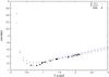 |
Fig. 1 Conversion factor between ROSAT and bolometric luminosities as a function of temperature. Red triangles are for metallicity of 0.1, blue diamonds are for metallicity of 0.5, black points represent the actual conversion factors used for the sample. |
The background treatment was performed as in Bharadwaj et al. (2014). The particle background was estimated using the stowed events files distributed within the CALDB. For the astrophysical background, we performed a simultaneous spectral fit to the Chandra data and the RASS data (provided by Snowden’s webtool1). The background components were an absorbed power law with a spectral index of 1.41 for unresolved AGN, an absorbed astrophysical plasma emission code (APEC) model for Galactic halo emission, and an unabsorbed APEC model for Local Hot Bubble emission (Snowden et al. 1998). The RASS data were taken from an annulus far away from the group centre, where no group emission would be present. The group emission was modelled with an absorbed APEC model, with the temperature and abundance free to vary. All absorption components were linked and modelled with the phabs model, and NH values were taken from a webtool2, which follows the method described in Willingale et al. (2013). In some cases, these were found to be too low, and they were left as free parameters in the spectral fit. This has the effect of lowering the temperatures, with the largest change being in the order of 6%. The Anders & Grevesse (1989) abundance table and AtomDB 2.0.2 was used throughout. Since we wished to study the bolometric LX − T relation, we had to convert the quoted ROSAT (0.1–2.4 keV) luminosities in Eckmiller et al. (2011) to the bolometric band (0.01–40 keV), for which we used the program Xspec. Using an APEC model frozen to the best-fit temperature, abundance, and redshift for the groups, we calculated the luminosities in the ROSAT band and the bolometric band. The ratio of the ROSAT and bolometric LX gives us the conversion factor to transform between the two luminosities. This conversion factor largely depends on the temperature and slightly on the abundance of the ICM (Fig. 1). Given that most groups from the eROSITA all-sky survey would likely lack sufficient counts to resolve the core, we did not use core-excised luminosities. The temperatures, luminosities, and NH values are listed in Table 1.
Temperatures, bolometric luminosities, and NH for the galaxy groups.
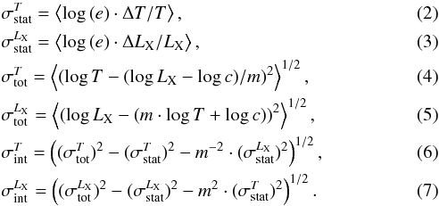
For getting the slope and normalisation of the best-fit scaling relation, we used the bivariate correlated errors and intrinsic scatter (BCES) (Y|X) code by Akritas & Bershady (1996). The fits were performed in log space for the fitting function:  (1)We also calculated statistical and intrinsic scatters with the following formulae3:
The fits were performed for five different cases, which are presented in Table 2. To test the effects of ICM cooling on the relation, we sub-divided the sample into the SCC and non-strong cool core (NSCC; CCT ≥ 1 Gyr) cases. To test the effects of AGN feedback, we classified the systems as those with and without a central radio source (CRS and NCRS respectively), a CRS representative of the presence of a radio loud AGN.
Observed bolometric relation.
2.3. Bias correction
Observed scaling relations can be affected by various selection biases, chief among which is the Malmquist bias. The Malmquist bias is the preferential detection of brighter objects for e.g. a given temperature, in a flux-limited sample due to intrinsic scatter. It is an effect that has been shown to affect scaling relations, namely resulting in higher observed normalisations as compared to the actual normalisations in scaling relations for clusters (e.g. Ikebe et al. 2002; Stanek et al. 2006; Pratt et al. 2009; Mantz et al. 2010; Lovisari et al. 2014). In this sample, we have applied an additional luminosity cut which could further contribute to the bias. Thus, in order to determine the “true” relation, one has to correct for these biases. To do this, we undertook simulations, the procedure of which we describe below.
For the simulations, we randomly generated samples of groups with temperatures between 0.6 and 3.6 keV. These groups were assigned luminosity distances such that the number of objects scaled as  , between redshifts of 0.01 and 0.2, and temperatures corresponding to the X-ray temperature function (the XTF, Markevitch 1998, given by dN/ dV ~ T-3.2). Using different combinations of slopes, normalisations, and scatters, we assigned luminosities to these temperatures. The intrinsic scatter about LX is log-normal and was introduced as such. Measurement errors were included for both LX and T, which corresponded to the observed statistical scatter. For each set of parameters, we generated 100 samples and applied a flux cut of 2.5 × 10⁻¹² erg s-1 cm-2 and an upper luminosity cut of (both in the ROSAT band) to simulate the selection criteria, with each sample containing between 20–30 objects, similar to the actual group sample used in the study. To determine the best set of parameters, we defined a chi-squared:
 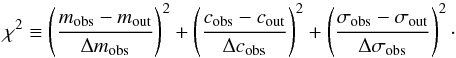 (8)Here m is slope, c is normalisation, σ is the intrinsic scatter in luminosity. Obs are the observed parameters, out is the output given by the simulation. The deltas represent the measured errors, from the BCES fit. For the scatter, we assumed that
  . Changing this value from 5 to 20% does not alter the results significantly. An example of this simulation is shown in Fig. 2.
Scaling relations for different cases, e.g. SCC and NSCC groups, may differ, therefore selection effects may differ for the different cases as well, making it imperative to determine bias corrections for the individual sub-cases. To do this, fresh simulations were run with the fractions of SCC/NSCC objects, and CRS/NCRS objects fixed to the observed values noted in Bharadwaj et al. (2014). We note that small changes in the SCC/NSCC fractions and the CRS/NCRS fractions do not drastically affect the determination of the bias-corrected slopes, normalisations, and scatters for the group sample.
Note that, despite our concerted efforts to correct for the selection biases, due to the incomplete nature of this sample compiled from the Chandra archives, we do not rule out the possibility of a potential “archival bias”, which could have a bearing on the results and which we cannot correct for.
2.4. Cluster comparison sample
To compare our results for groups to galaxy clusters, we decided to use the HIFLUGCS galaxy clusters (Reiprich & Böhringer 2002), a flux-limited sample with ROSAT (0.1–2.4 keV) flux ≥2 × 10-11 erg s-1 cm-2. For this study, we took the bolometric X-ray luminosities and virial temperatures quoted in Mittal et al. (2011). Since the temperatures were determined with CALDB version 3 (3.2.1) versus version 4 for the galaxy groups, we converted the quoted temperatures using the scaling relation quoted in Mittal et al. (2011), namely:  (9)Using this scaling relation has the effect of lowering the temperature, thereby raising the normalisation and steepening the observed cluster LX − T relation. The change in slope and normalisation, however, are within the errors of that obtained with the older temperatures. Since the groups and the cluster samples have different selection criteria, bias corrections were performed for clusters as well, using the above flux limit to compare results accurately. For the sub-samples, we took the SCC/NSCC fraction and the CRS/NCRS fraction for the clusters from Hudson et al. (2010) and Mittal et al. (2009), respectively.
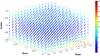 |
Fig. 2 Slopes, normalisations, and intrinsic scatter for the “all groups” case. The plot is colour-coded to represent the value of chi-squared. |
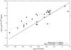 |
Fig. 3 Observed and bias-corrected LX − T relation for galaxy groups. The dotted line is the observed scaling relation and the solid line is the bias-corrected scaling relation. |
Bias corrected, bolometric LX − T relation for groups, and clusters.
3. Results and discussion
3.1. Observed, bias-uncorrected LX − T relation
The fit results for the observed data sets (both groups and clusters) are shown in Table 2. For all groups, the best-fit results are shown in Fig. 3.
The very first observation that one makes on comparing the observed LX − T relation of groups to clusters is the flattening of the slope when one enters the group regime. Additionally, we observe that for most cases, the slope of the observed LX − T relation is consistent with the self-similar value of 2 expected for clusters within the errors. As we demonstrate in Sect. 3.2, this is due to the selection criteria applied to construct this sample, and is not a property of the underlying group population. Additionally, the observed LX − T relation for the SCC groups shows indications of being higher in normalisation (by a factor of ~2) and having a steeper slope as compared to the NSCC groups. For groups with a CRS, there is an indication that the normalisation is lower than for those groups without a CRS.
The statistical scatters in the temperature for both groups and clusters are in good agreement, but for the luminosity, we see an increase by around a factor of 5 as we go from the cluster to the group regime. This is expected, as groups, being low surface brightness systems, have a much larger error in their luminosity than is the case for clusters. Additionally, the luminosities for the galaxy groups come from the RASS data with very short exposure times, versus that of the clusters, which come from ROSAT position sensitive proportional counter (PSPC) pointed observations with much larger exposure times, leading to a much more precise determination of the cluster luminosities.
3.2. Bias-corrected LX − T relation
We tabulate the bias corrected LX − T relation for both groups and clusters in Table 3. As pointed out before, this is the first attempt to present a bias-corrected bolometric LX − T relation for groups including their cool-core and central AGN properties, making comparisons between groups and clusters a lot easier than before.
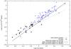 |
Fig. 4 Observed and bias-corrected LX − T relations. Clusters are represented by blue points and groups are represented by black points. Dotted line is observed relation for groups, solid line is bias-corrected relation for groups, dot-dash line is bias-corrected relation for clusters. |
Our very first observation is that correcting for selection effects has a significant impact on the LX − T relation for the galaxy groups. Over most of the temperature range covered by the group sample, the bias corrected relation results in a lower LX for a given T, and the bias-corrected slope steepens significantly from 2.17 to 3.20 (Fig. 3). With the corrections in place, the value of our slope agrees well with previous bolometric LX − T slopes for galaxy groups observed for incomplete samples (e.g. Osmond & Ponman 2004), but is much lower than reported slopes of ~5 (Helsdon & Ponman 2000; Xue & Wu 2000 at >5σ significance). The value of the corrected slope for groups shows indications of a steepening compared to clusters, but the two slopes are consistent within the errors (Fig. 4, Table 3). Qualitatively our results show the same trend as reported recently by Lovisari et al. (2014).
Sub-classifying the sample yields more interesting features. The LX − T relation for the SCC and CRS groups is by far the steepest with the SCC groups having the highest normalisation for all the sub-samples at 3 keV. The slope of the bias-corrected LX − T relation for the SCC groups is steeper than the NSCC slope by 43% and higher in normalisation by a factor of ~3 at 3 keV (Fig. 5). The normalisations for the CRS groups and NCRS groups are in good agreement (within 17%, ignoring the errors), but there are indications of marginal steepening of the slopes for the CRS systems, albeit the large error bars make it hard to confirm. The bias-corrected slopes of most of the sub-samples for the groups and clusters are once again consistent within the errors. These numbers suggest a rather complicated scenario for the group regime and we discuss this in Sect. 3.3.
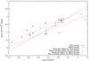 |
Fig. 5 Observed and bias-corrected LX − T relation for SCC and NSCC groups. Blue dotted line represents observed relation for SCC groups, blue solid line represents bias-corrected relation for SCC groups, red dotted line represents observed relation for NSCC groups, red solid line represents bias-corrected relation for NSCC groups. |
Our attempt to identify the bias-corrected scatter vs. the observed scatter for LX to our best knowledge is a first for the LX − T scaling relation. Interestingly, while the observed and the bias-corrected scatter for the complete cluster sample agree within 10%, the bias-corrected scatter for groups is higher by 35% as compared to the observed scatter. This statement also holds true qualitatively for most of the sub-samples that we fit here. The reason behind this could simply be due to the applied upper luminosity cut to select the group sample. The corrected intrinsic scatter increases by 19% as one moves down from the cluster to the group regime, with the largest change in intrinsic scatter between groups and clusters observed for the CRS case (~38%). We have demonstrated for the first time, that the bias-corrected intrinsic scatter in LX seems to increase from the cluster to the group regime. This would indicate a stronger impact of non-gravitational processes on the group regime than the cluster regime, as one would expect. Interestingly, this conclusion of ours is somewhat different to the results of Lovisari et al. (2014), who conclude that the scatter decreases as one goes from the cluster to the group regime. We point out that their conclusion is based on the observed scatter as they do not explicitly try to obtain a bias-corrected scatter as we have done in this study. Nevertheless, the small sample sizes in both studies, the choice of X-ray luminosities (ROSAT band vs. bolometric band), the potential archival bias in our study, and different techniques in performing the bias correction could all have a potential impact on the determination of the “true” scatter.
Our simulations clearly demonstrate that selection criteria employing a flux and luminosity cut have a stronger impact on the LX − T relation, particularly on the slope, than those with just a simple flux cut, as in e.g. the HIFLUGCS cluster sample. Additionally, we have also demonstrated that the bias corrections for sub-samples, especially SCC and NSCC sub-samples are not identical and have to be determined individually.
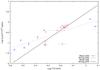 |
Fig. 6 The LX − T relation for sub-samples divided on the basis of the median radio luminosity of the CRS. Blue points (“weak” CRS) represent those groups that have a CRS with total radio luminosity less than the median radio luminosity, while red points represent those groups with a CRS greater than or equal to the median radio luminosity. |
3.3. A complete picture of the LX − T relation
When one wishes to interpret observational results for scaling relations, a good starting point is to look at existing results from simulations. In recent times, the introduction of sophisticated code, which accounts for non-gravitational processes such as cooling and feedback, have made simulations much more accurate than before. It is all but clear that only simulation recipes with some form of AGN feedback can mitigate excessive gas cooling and high star formation rates that are inconsistent with observations (e.g. Borgani et al. 2004). Recent results by e.g. Puchwein et al. (2008) and McCarthy et al. (2010) argue that an LX − T relation consistent with observations is obtained for groups only with AGN feedback. This simplified picture would seem to solve all problems, but observations seem to point to a more complex scenario.
Interpreting the high normalisations of the SCC groups is relatively straightforward; these are systems with the most centrally dense cores, and since the emissivity scales as the density squared, there is a boost given to their X-ray luminosities leading to a higher normalisation in the LX − T relation compared to other sub-samples. The steepening could be explained as a higher increase in X-ray luminosity for relatively high temperature SCC groups (≥1 keV), which probably continues to decrease as we go down the temperature scale. The relatively low X-ray luminosity for the NSCC groups, which are WCC and NCC groups, is an indication that there is not strong cooling going on in these systems. It could also indicate the further influence of AGN feedback (particularly for the NCC groups), which suppresses the X-ray luminosity, though we do wish to point out that not all WCC groups harbour a CRS.
This brings us to our next point of discussion, namely the LX − T relation for those groups with and without a CRS. As the slopes and normalisations for the CRS and the NCRS are both consistent within the errors for the CRS and the NCRS cases, we tried to see if divisions based on the morphology of the CRS could unravel some features. Dividing the groups between those with an CRS that show extended radio emission and those with CRSs that show only central emission based on a visual inspection of the radio contours (Appendix C of Bharadwaj et al. 2014), we observe that the former has a much steeper slope than the latter (3.64 ± 1.21 vs. 2.07 ± 0.31). Taking this one step further, we fit the LX − T relation for two more sub-samples; this time dividing the sample on the basis of the median radio luminosity of the CRSs (Fig. 6). Once again, we observe that the groups with a “strong” radio source (greater than or equal to the median radio luminosity) have a much steeper scaling relation (4.11 ± 1.38 vs. 1.96 ± 0.31) than those with “weak” radio sources. Qualitatively, both these results are in agreement with Magliocchetti & Brüggen (2007) who find a much steeper slope for objects with extended radio sources (~4) than for radio sources with point-like emission. The mean radio output of the SCC groups CRS is a factor of 34 lower than the NSCC groups CRS, which could indicate that AGN activity is weaker in SCC groups than the NSCC groups, assuming the radio luminosity is a good indicator of AGN activity. This would be very much in line with simulation results by Gaspari et al. (2011, 2014) who argue that AGN feedback in galaxy groups must be self-regulated with low mechanical efficiencies, and is a fundamental requirement for the preservation of the cool core. Moreover, in this particular group sample, 60% of the groups with a “strong” CRS are NSCC groups, while 60% of the groups with a “weak” CRS are SCC groups. This could be an indication that the more powerful radio AGN are preferentially located in NSCC groups rather than SCC groups. These conclusions are subject to selection effects, and more robust results would require a much larger, complete group sample, backed by radio data down to lower frequencies and more homogeneous flux limits.
4. Summary
With a sample of 26 galaxy groups, we studied the effects of ICM cooling, AGN feedback, and selection effects on the LX − T relation for the galaxy group regime. The main results of this study can be summarised as follows:
-
The observed LX − T relation for groups is significantly affected by selection effects that impact the slope, normalisation, and the intrinsic scatter in LX and requires bias corrections. We also conclude that SCC groups require a different bias correction than NSCC groups.
-
The bias-corrected slope of the LX − T relation for groups obtained after correcting for selection effects shows indications of steepening, but is consistent within errors to the bias-corrected slope of the clusters.
-
The SCC groups have the highest normalisation and the steepest slope for the scaling relation. This is attributed to the enhanced luminosities of these systems.
-
The bias-corrected intrinsic scatter in LX seems to generally increase as we enter the group regime. Additionally, for groups the observed intrinsic scatter is lower than the bias-corrected scatter obtained from simulations for most cases.
-
Subject to selection effects, we see indications of a steepening of the scaling relation for those groups that have a CRS radio luminosity greater than the median, and speculate that such relatively powerful CRSs are preferentially located in NSCC groups.
In short, we have demonstrated that the behaviour of the LX − T relation in groups is similar (e.g. the slopes) and yet different (e.g. intrinsic scatter in LX) to that in clusters. The next step towards having a survey ready LX − T relation would be to account for every process at work in galaxy groups, their effect
on the slopes and normalisations, and their contribution to the overall scatter. Quantifying these processes will be a challenge. As we have pointed out, objectively selected, large samples of groups, particularly to much lower temperatures (<1 keV) with good quality X-ray data and without potential archival bias, would be of paramount importance. Additionally, we expect more features to be obtained when we sub-classify these potential group samples into SCC, WCC, and NCC classes and sub-classes thereof. This is a project that we hope to pursue in the near future.
In log space, errors are expressed as Δlog x = log (e) (x+ − x−) / (2x) where x+ and x− are the upper and lower boundary of the error range of the quantity x.
Acknowledgments
The authors would like to thank the anonymous referee who provided useful comments which helped improve the quality of the work. V.B. would like to thank Gerrit Schellenberger for useful discussions and for providing a C version of the BCES code. V.B. acknowledges support from grant RE 1462/6. L.L. acknowledges support by the DFG through grant LO2009/1-1, RE 1462/6 and by the Transregional Collaborative Research Centre TRR33 “The Dark Universe” (project B18). T.H.R. acknowledges support from the DFG through the Heisenberg research grant RE 1462/5.
References
- Akritas, M. G., & Bershady, M. A. 1996, ApJ, 470, 706 [NASA ADS] [CrossRef] [Google Scholar]
- Allen, S. W., Schmidt, R. W., & Fabian, A. C. 2001, MNRAS, 328, L37 [NASA ADS] [CrossRef] [Google Scholar]
- Anders, E., & Grevesse, N. 1989, GCA, 53, 197 [Google Scholar]
- Arnaud, M., & Evrard, A. E. 1999, MNRAS, 305, 631 [NASA ADS] [CrossRef] [Google Scholar]
- Bharadwaj, V., Reiprich, T. H., Schellenberger, G., et al. 2014, A&A, 572, A46 [NASA ADS] [CrossRef] [EDP Sciences] [Google Scholar]
- Böhringer, H., Voges, W., Huchra, J. P., et al. 2000, ApJS, 129, 435 [NASA ADS] [CrossRef] [Google Scholar]
- Böhringer, H., Schuecker, P., Guzzo, L., et al. 2004, A&A, 425, 367 [NASA ADS] [CrossRef] [EDP Sciences] [Google Scholar]
- Borgani, S., Murante, G., Springel, V., et al. 2004, MNRAS, 348, 1078 [NASA ADS] [CrossRef] [Google Scholar]
- Borm, K., Reiprich, T. H., Mohammed, I., & Lovisari, L. 2014, A&A, 567, A65 [NASA ADS] [CrossRef] [EDP Sciences] [Google Scholar]
- Eckmiller, H. J., Hudson, D. S., & Reiprich, T. H. 2011, A&A, 535, A105 [NASA ADS] [CrossRef] [EDP Sciences] [Google Scholar]
- Eke, V. R., Navarro, J. F., & Frenk, C. S. 1998, ApJ, 503, 569 [NASA ADS] [CrossRef] [Google Scholar]
- Gaspari, M., Brighenti, F., D’Ercole, A., & Melioli, C. 2011, MNRAS, 415, 1549 [NASA ADS] [CrossRef] [Google Scholar]
- Gaspari, M., Brighenti, F., Temi, P., & Ettori, S. 2014, ApJ, 783, L10 [NASA ADS] [CrossRef] [Google Scholar]
- Giodini, S., Pierini, D., Finoguenov, A., et al. 2009, ApJ, 703, 982 [NASA ADS] [CrossRef] [Google Scholar]
- Giodini, S., Lovisari, L., Pointecouteau, E., et al. 2013, Space Sci. Rev., 177, 247 [NASA ADS] [CrossRef] [Google Scholar]
- Helsdon, S. F., & Ponman, T. J. 2000, MNRAS, 315, 356 [NASA ADS] [CrossRef] [Google Scholar]
- Hudson, D. S., Mittal, R., Reiprich, T. H., et al. 2010, A&A, 513, A37 [NASA ADS] [CrossRef] [EDP Sciences] [Google Scholar]
- Ikebe, Y., Reiprich, T. H., Böhringer, H., Tanaka, Y., & Kitayama, T. 2002, A&A, 383, 773 [NASA ADS] [CrossRef] [EDP Sciences] [Google Scholar]
- Jarrett, T. H., Chester, T., Cutri, R., et al. 2000, AJ, 119, 2498 [NASA ADS] [CrossRef] [Google Scholar]
- Lovisari, L., Reiprich, T., & Schellenberger, G. 2014, A&A, in press, DOI: 10.1051/0004-6361/201423954 [Google Scholar]
- Magliocchetti, M., & Brüggen, M. 2007, MNRAS, 379, 260 [NASA ADS] [CrossRef] [Google Scholar]
- Mantz, A., Allen, S. W., Ebeling, H., Rapetti, D., & Drlica-Wagner, A. 2010, MNRAS, 406, 1773 [NASA ADS] [Google Scholar]
- Markevitch, M. 1998, ApJ, 504, 27 [NASA ADS] [CrossRef] [Google Scholar]
- McCarthy, I. G., Schaye, J., Ponman, T. J., et al. 2010, MNRAS, 406, 822 [NASA ADS] [Google Scholar]
- Merloni, A., Predehl, P., Becker, W., et al. 2012 [arXiv:1209.3114] [Google Scholar]
- Mittal, R., Hudson, D. S., Reiprich, T. H., & Clarke, T. 2009, A&A, 501, 835 [NASA ADS] [CrossRef] [EDP Sciences] [Google Scholar]
- Mittal, R., Hicks, A., Reiprich, T. H., & Jaritz, V. 2011, A&A, 532, A133 [NASA ADS] [CrossRef] [EDP Sciences] [Google Scholar]
- O’Hara, T. B., Mohr, J. J., Bialek, J. J., & Evrard, A. E. 2006, ApJ, 639, 64 [NASA ADS] [CrossRef] [Google Scholar]
- Osmond, J. P. F., & Ponman, T. J. 2004, MNRAS, 350, 1511 [NASA ADS] [CrossRef] [Google Scholar]
- Pillepich, A., Porciani, C., & Reiprich, T. H. 2012, MNRAS, 422, 44 [NASA ADS] [CrossRef] [Google Scholar]
- Ponman, T. J., Bourner, P. D. J., Ebeling, H., & Böhringer, H. 1996, MNRAS, 283, 690 [NASA ADS] [CrossRef] [Google Scholar]
- Pratt, G. W., Croston, J. H., Arnaud, M., & Böhringer, H. 2009, A&A, 498, 361 [NASA ADS] [CrossRef] [EDP Sciences] [Google Scholar]
- Predehl, P., Andritschke, R., Böhringer, H., et al. 2010, in SPIE Conf. Ser., 7732, 10 [Google Scholar]
- Puchwein, E., Sijacki, D., & Springel, V. 2008, ApJ, 687, L53 [NASA ADS] [CrossRef] [Google Scholar]
- Reiprich, T. H., & Böhringer, H. 2002, ApJ, 567, 716 [NASA ADS] [CrossRef] [Google Scholar]
- Skrutskie, M. F., Cutri, R. M., Stiening, R., et al. 2006, AJ, 131, 1163 [NASA ADS] [CrossRef] [Google Scholar]
- Snowden, S. L., Egger, R., Finkbeiner, D. P., Freyberg, M. J., & Plucinsky, P. P. 1998, ApJ, 493, 715 [NASA ADS] [CrossRef] [Google Scholar]
- Stanek, R., Evrard, A. E., Böhringer, H., Schuecker, P., & Nord, B. 2006, ApJ, 648, 956 [NASA ADS] [CrossRef] [Google Scholar]
- Sun, M., Voit, G. M., Donahue, M., et al. 2009, ApJ, 693, 1142 [NASA ADS] [CrossRef] [Google Scholar]
- Tinker, J., Kravtsov, A. V., Klypin, A., et al. 2008, ApJ, 688, 709 [NASA ADS] [CrossRef] [Google Scholar]
- Vikhlinin, A., Kravtsov, A., Forman, W., et al. 2006, ApJ, 640, 691 [NASA ADS] [CrossRef] [Google Scholar]
- Vikhlinin, A., Burenin, R. A., Ebeling, H., et al. 2009, ApJ, 692, 1033 [NASA ADS] [CrossRef] [Google Scholar]
- Willingale, R., Starling, R. L. C., Beardmore, A. P., Tanvir, N. R., & O’Brien, P. T. 2013, MNRAS, 431, 394 [NASA ADS] [CrossRef] [Google Scholar]
- Xue, Y.-J., & Wu, X.-P. 2000, ApJ, 538, 65 [NASA ADS] [CrossRef] [Google Scholar]
All Tables
All Figures
|
Fig. 1 Conversion factor between ROSAT and bolometric luminosities as a function of temperature. Red triangles are for metallicity of 0.1, blue diamonds are for metallicity of 0.5, black points represent the actual conversion factors used for the sample. |
| In the text | |
|
Fig. 2 Slopes, normalisations, and intrinsic scatter for the “all groups” case. The plot is colour-coded to represent the value of chi-squared. |
| In the text | |
|
Fig. 3 Observed and bias-corrected LX − T relation for galaxy groups. The dotted line is the observed scaling relation and the solid line is the bias-corrected scaling relation. |
| In the text | |
|
Fig. 4 Observed and bias-corrected LX − T relations. Clusters are represented by blue points and groups are represented by black points. Dotted line is observed relation for groups, solid line is bias-corrected relation for groups, dot-dash line is bias-corrected relation for clusters. |
| In the text | |
|
Fig. 5 Observed and bias-corrected LX − T relation for SCC and NSCC groups. Blue dotted line represents observed relation for SCC groups, blue solid line represents bias-corrected relation for SCC groups, red dotted line represents observed relation for NSCC groups, red solid line represents bias-corrected relation for NSCC groups. |
| In the text | |
|
Fig. 6 The LX − T relation for sub-samples divided on the basis of the median radio luminosity of the CRS. Blue points (“weak” CRS) represent those groups that have a CRS with total radio luminosity less than the median radio luminosity, while red points represent those groups with a CRS greater than or equal to the median radio luminosity. |
| In the text | |
Current usage metrics show cumulative count of Article Views (full-text article views including HTML views, PDF and ePub downloads, according to the available data) and Abstracts Views on Vision4Press platform.
Data correspond to usage on the plateform after 2015. The current usage metrics is available 48-96 hours after online publication and is updated daily on week days.
Initial download of the metrics may take a while.