| Issue |
A&A
Volume 573, January 2015
|
|
|---|---|---|
| Article Number | A104 | |
| Number of page(s) | 9 | |
| Section | The Sun | |
| DOI | https://doi.org/10.1051/0004-6361/201424561 | |
| Published online | 06 January 2015 | |
The evolution of the emission measure distribution in the core of an active region
1 Department of Applied Mathematics and Theoretical Physics, University of Cambridge, Wilberforce Road, Cambridge CB3 0WA, UK
e-mail: This email address is being protected from spambots. You need JavaScript enabled to view it.
2 Inter-University Centre for Astronomy and Astrophysics, Post Bag-4, Ganeshkhind, 411007 Pune, India
Received: 8 July 2014
Accepted: 22 October 2014
Abstract
We study the spatial distribution and evolution of the slope of the emission measure (EM) between 1 MK and 3 MK in the core of the active region (AR) NOAA 11193, first when it appeared near the central meridian and then again when it reappeared after a solar rotation. We use observations recorded by the Extreme-ultraviolet Imaging Spectrometer (EIS) aboard Hinode, with a new radiometric calibration. We also use observations from the Atmospheric Imaging Assembly (AIA) aboard the Solar Dynamics Observatory (SDO). We present the first spatially resolved maps of the EM slope in the 1–3 MK range within the core of the AR using several methods, either from approximations or from the differential emission measure (DEM). A significant variation of the slope is found at different spatial locations within the active region. We selected two regions that were not greatly affected by lower temperature emission along the line of sight. We found that the EM had a power law of the form EM ∝ Tb, with b = 4.4 ± 0.4, and 4.6 ± 0.4, during the first and second appearance of the active region, respectively. During the second rotation, line-of-sight effects become more important, although difficult to estimate. We found that the use of the ground calibration for Hinode/EIS and the approximate method to derive the EM, used in previous publications, produce an underestimation of the slopes. The EM distribution in active region cores is generally found to be consistent with high frequency heating, and does not change much during the evolution of the active region.
Key words: Sun: atmosphere / Sun: corona / methods: observational / methods: data analysis
© ESO, 2015
1. Introduction
The solution to the long standing problem of solar coronal heating remains elusive despite major advances in observational and theoretical capabilities over the last few decades (see Klimchuk 2006 for a review). We now know that active regions generally comprise a variety of structures which are broadly classified as warm loops [T ≃ 1 MK]; fan loops [T< 0.8 MK]; mostly emanating from sunspots, and hot loops [T ≃ 3 MK] in the cores of active regions. Additionally, it is also known that there is significant unresolved emission in the 1–3 MK range (see e.g. Del Zanna & Mason 2003; Viall & Klimchuk 2012; Del Zanna 2013b; Subramanian et al. 2014). Therefore, any theory for coronal heating must explain the emission from these different kinds of loops as well as the diffuse emission.
A clear understanding of the thermal distribution and timescale of energy release in coronal structures reveals information regarding the heating mechanisms in that particular structure. There is an ongoing debate in the current literature as to whether the heating is low- or high-frequency. High (low) frequency heating occurs when the duration between successive heating events is smaller (larger) than the cooling time (Tripathi et al. 2011). In the high-frequency heating scenario, the plasma does not have enough time to cool sufficiently and produces a narrow emission measure (EM) distribution with a steep slope b [EM(T) ∝ Tb] in the 1–3 MK range. However, in the low frequency heating scenario, since the time duration is larger than the cooling time, the plasma has sufficient time to cool down before being heated again. Hence, there would be a substantial amount of material at cooler temperatures giving rise to comparatively shallower slopes (see e.g. Mulu-Moore et al. 2011; Tripathi et al. 2011; Bradshaw et al. 2012; Cargill 2014 and references therein). Generally, the models predict that low-frequency nanoflares can only account for slopes b that are below 3.
The emission of the ≃1 MK warm loops observed in EUV with the Extreme-ultraviolet Imaging Telescope (EIT; Delaboudinière et al. 1995) on board SoHO, the Transition Region And Coronal Explorer (TRACE; Handy et al. 1999), the Extreme-Ultraviolet Imaging Spectrometer (EIS; Culhane et al. 2007) abroad Hinode, and most recently by the Atmospheric Imaging Assembly (AIA; Lemen et al. 2012) on board the Solar Dynamics Observatory (SDO) is generally explained by low frequency heating (see e.g. Warren et al. 2003, 2008; Winebarger et al. 2003; Tripathi et al. 2009; Ugarte-Urra et al. 2009; Klimchuk 2009). The heating of the hot loops in the core of the active regions has been, however, a matter of much debate (see e.g. Tripathi et al. 2010b,a, 2011, 2012; Warren et al. 2010, 2011, 2012; Winebarger et al. 2011, 2013; Viall & Klimchuk 2011; Dadashi et al. 2012; Schmelz & Pathak 2012; Ugarte-Urra & Warren 2012). One issue that is still not clear is the amount of hot plasma above 3 MK; EUV and X-ray spectroscopic observations indicate that the cores of quiescent ARs have very little hot plasma (see Del Zanna 2013b; Del Zanna & Mason 2014 and references therein), a topic that we do not discuss here.
This paper focuses on the slopes in the 1–3 MK temperature range. Recent studies used Hinode EIS observations of the cores of active regions, avoiding moss emission. For example, Warren et al. (2011) studied an inter-moss region and found an EM distribution that can be approximated by EM ∝ T3.26. For a different active region Winebarger et al. (2011) found a similar power-law slope (EM ∝ T3.2). However, Tripathi et al. (2011) found EM distributions with a power-law slope of approximately 2.4 for several inter-moss regions of two active regions. A different method was used. Warren et al. (2012) studied the EM distribution in the cores of 15 active regions and found EM distributions that had a range of slopes, between 2 and 5.
Two questions naturally arise. Are these slopes different depending on the AR? Do they change during the lifetime of an active region? The general evolution of an active region has been known for a long time for example from Skylab observations (see Sheeley 1981); however, a quantitative analysis on small spatial scales was not available. Recently, Ugarte-Urra & Warren (2012) studied two active region cores at several instances during their life time, with Hinode/EIS, STEREO/EUVI, and SDO/AIA. They found that the EM at 4 MK normally declines with time, following its suggested relationship with the magnetic flux (Warren et al. 2012). However, they also found an enhancement with time in the EM at lower temperatures, 0.6–0.9 MK. Their results suggest that both low and high frequency heating can occur in active region cores during the lifetime of an active region. The EM enhancement at lower temperatures could also be interpreted as dominance of low frequency heating events during the later part of an active regions’ life. Similarly, Schmelz & Pathak (2012) studied eight inter-moss regions in five different active regions (some overlapping with those studied by Warren et al. 2012). They combined Hinode EIS and XRT observations to better constrain the high temperature component of the EM. In addition, they estimated the age of the active region, although they did not actually track the same active region during two rotations. They concluded that their results were consistent with older active regions being more likely dominated by steady heating (high frequency impulsive heating) and younger regions showing more evidence of low frequency impulsive heating.
We believe that it is important to track the evolution of the same active region. In this paper we present Hinode/EIS and SDO/AIA observations of the core of the same active region at two instances during its life time, once when it appeared on disk and again when the active region was seen after one solar rotation.
Three questions naturally arise. 1) How do the slopes vary within the active region? We discuss possible methods of obtaining the slopes for each observed pixel, from simple fast methods to more complex methods, and we present the results. 2) How does the spatial resolution affect the results? We complement the Hinode/EIS observations with the much higher-resolution SDO/AIA data, and compare the slopes obtained from the two instruments. 3) Given that different methods have been used in the literature to derive the DEM and EM, how do the slopes depend on the method used? We compare the results obtained for different methods.
Guennou et al. (2013) has recently highlighted that atomic data uncertainties affect the estimation of the slopes. We show that another important issue that was neglected in previous literature is the EIS radiometric calibration, which has recently been revised (Del Zanna 2013a).
The paper is organised as follows: in Sect. 2 we describe the observations of the active region, in Sect. 3 we review the different methods we adopt, and in Sect. 4 we describe our data analysis and results, followed by a summary and conclusions in Sect. 5.
2. Observations
In the current analysis we have used observations recorded by EIS aboard Hinode and AIA aboard SDO. EIS provides high resolution spectra of the Sun in two wavelength bands, 170–211 Å, and 246–292 Å (Culhane et al. 2007), with an effective spatial resolution of about 3′′. AIA provides high-resolution imaging observations (with about 1′′ resolution, 0.6 arcsec/pixel) in 6 extreme-ultraviolet channels with high cadence (Lemen et al. 2012).
We believe that line-of-sight effects can play an important role in estimating the slope of the EM, so we have searched for an active region that was observed when it was close to the central meridian, and were careful to select areas in the hot core loops which are free from contamination by low-lying moss regions. We have also analysed simultaneous SDO/AIA and Hinode/EIS observations to determine the EIS pointing and obtain high-resolution information. For this study we have selected the active region NOAA 11193. This AR was first observed near the central meridian on Apr. 19, 2011 and then again on May 16 and 17, 2011 during its second passage from the central meridian on the visible solar disk. STEREO EUVI images indicate that the AR emerged on Apr. 10, i.e. it was already 9 days old at first meridian passage.
The AIA data have been processed in the following way (see Del Zanna et al. 2011; and Del Zanna 2013b, for details). We took the full-disk AIA data and adjusted the plate scale. We then corrected for the AIA stray light using the results of Poduval et al. (2013). We note that the correction for the stray light enhances the contrast between the loop structures and the background. In order to align AIA and EIS accurately, the AIA images were then reduced to the lower spatial and temporal resolution of the EIS data for a direct comparison, i.e. to find the EIS pointing. The AIA and EIS comparisons show, as in previous cases we have analysed (Del Zanna et al. 2011; Del Zanna 2013b), that the displacement in the E-W direction of the EIS slit between different exposures is not equal to the nominal value. For example, a step of 2′′ is in fact a step of 1.8′′.
AIA images of the active region NOAA 11193 are shown in Fig. 1, when it was close to the central meridian on 19 April 2011 and on 16 May 2011. The images are shown on the same intensity scale to show how much the active region has changed. The changes are typical of most active regions. To actually interpret the emission in the SDO AIA bands, it is necessary to keep in mind that all the AIA bands are highly multi-thermal, as described in detail in O’Dwyer et al. (2010), Del Zanna et al. (2011, 2013). The core of the AR in the 335 Å band is dominated by the Fe xvi 335.41 Å line (Del Zanna 2013b), which is formed at 3 MK, hence clearly shows the hot core loops. There is a significant reduction in this 3 MK emission during the second rotation. The brightest emission at 1–2 MK is in the low-lying moss regions, the footpoint regions of hot AR loops (see e.g. Tripathi et al. 2010a, and references therein). The moss is clearly visible in the 193 Å band, which in these locations is dominated by Fe xii emission (Del Zanna 2013b). The moss emission is significantly reduced during the second rotation.
The ≃1 MK warm loops are already fully developed by the 19 April 2011, and are clearly visible in the 171 Å channel, dominated by Fe ix 171 Å, which is formed over a relatively broad temperature range centred around log T = 5.85, as discussed in Del Zanna et al. (2011). The warm loops that are outside the AR core become much stronger during the second rotation.
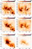 |
Fig. 1 AIA negative images of active region NOAA 11193 when it first appeared on the visible solar disk near the central meridian on Apr. 19, 2011 (left) and during the second rotation on May 17, 2011 (right). The intensities are DN/s, and the images of the two dates are shown on the same intensity scale and field of view. Coordinates are arcseconds from Sun centre. |
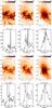 |
Fig. 2 AIA (DN/s, first and second row) and EIS (radiances in phot cm-2 st-1 s-1, third and fourth row) negative images on Apr. 19, 2011. The arrows indicate the AR core region selected for DEM analysis. The bottom plots show the profiles of the intensities along this vertical line. The dashed vertical lines in the bottom plots indicate the region selected for DEM analysis. |
The EIS observation sequence for the 19 April 2011 (HPW021 VEL 240 × 512v1) used the 1′′ slit with an exposure time of 60 s. The EIS raster started at 12:30:27 UT and finished at 14:34:14 UT. The raster was 240′′ wide and used a slit length of 512′′. For the second rotation of the active region NOAA 11193 we have chosen a full spectral atlas observation made on 17 May 2011. The EIS raster started at 00:48 UT and finished one hour later, at 01:50 UT. We designed this study to have a good signal-to-noise ratio, using the 2′′ slit, an exposure time of 60 s, and the full spectral range of EIS. We used custom-written software for the EIS data analysis. For details see Del Zanna (2013b).
Figure 2 shows a selection of AIA and EIS line intensity images, in the core of the AR, with profiles of the intensities across the AR on Apr. 19, 2011. The AIA images are 1 min averages at 13:30 UT. Figure 3 shows similar images for the 17 May 2011 observation, i.e. 1 min averages at 01:06 UT. The AIA images, thanks to their higher spatial and temporal resolution, show a much higher spatial variability.
To perform the DEM analysis for the first rotation we selected a region, indicated by the vertical lines in Fig. 2 (solar Y = 360), where we avoided, as much as possible, background contamination from the bright moss regions. The intensities in the EIS lines formed around 3 MK (e.g. Fe xvi) are much stronger in the core than in the surroundings, so are not affected by background contamination. There is, however, significant intensity in lines formed around 1 MK (e.g. Fe ix). The higher-resolution AIA 171 Å image clearly shows that some of the unresolved low temperature emission observed by EIS is due to the lower resolution of the spectrometer. Some low temperature (1 MK) emission is however also present in the AIA images, as found in other AR observations (Del Zanna 2013b). Whether this 1 MK emission is physically related (in terms of nanoflare storm) with the 3 MK emission is an open question that is not easy to answer. Estimating an appropriate background is also quite difficult, so we are providing the results without subtracting a background. Clearly, any slope obtained by EIS in the 1–3 MK range is bound to be a lower limit to the actual slope.
For the second rotation (see Fig. 3), we selected again a region where the 3 MK emission (e.g. Fe xvi) is strongest. Moss regions (strong in Fe xii and AIA 193 Å) were avoided. The intensity in EIS lines formed around 1 MK (e.g. Fe ix) is low, but similar to that of nearby regions. The AIA 171 Å image clearly shows this time that this 1 MK emission is originating from underlying cool loops that connect the two moss regions. Again, it is not clear if this cool emission is at all related to the 3 MK emission, so also in this case we are providing the results without subtracting a background, and the slope obtained from the EIS lines is bound to be a lower limit to the actual one.
3. Emission measure methods
We recall that the intensity of an optically thin line can be expressed as an integral along the line of sight  (1)where Ab is the elemental abundance, and G(Ne,Te) is the contribution function of the spectral line. G(Ne,Te) has a very strong dependence on temperature, and a negligible dependence on the electron number density, Ne, for a certain range of densities, if the appropriate line is chosen. Considering only such lines, and assuming that a unique relationship exists between Ne and Te, we define
 ![Mathematical equation: \begin{eqnarray} {\rm DEM} (T) = ~N_{\rm e} N_{\rm H} \frac{{\rm d}h}{{\rm d}T} \quad~~~\left[{\rm cm}^{-5}\,{\rm K}^{-1}\right] \end{eqnarray}](/articles/aa/full_html/2015/01/aa24561-14/aa24561-14-eq21.png) (2)as the column differential emission measure (DEM) of the plasma, which gives an indication of the amount of plasma along the line of sight that is emitting the radiation observed at a temperature between T and T + dT. The DEM by definition is a continuous distribution in a range of temperatures.
(2)as the column differential emission measure (DEM) of the plasma, which gives an indication of the amount of plasma along the line of sight that is emitting the radiation observed at a temperature between T and T + dT. The DEM by definition is a continuous distribution in a range of temperatures.
The DEM inversion is an ill-posed problem with various complexities associated, see e.g. (Craig & Brown 1976, 1986; Judge et al. 1997; Del Zanna 1999; Del Zanna et al. 2002) and references therein for details.
We have seen in previous studies that the methods of the inversion normally provide similar results, if the DEM is relatively well constrained and the same input parameters/temperature range is adopted (see e.g. Del Zanna et al. 2011; O’Dwyer et al. 2014; Del Zanna & Mason 2014). However, to assess the sensitivity of the present results to the method adopted, we have run three different DEM methods: the spline method described in Del Zanna (1999); the Markov chain Monte Carlo method of Kashyap & Drake (1998; MCMC_DEM); and the XRT_DEM_ITERATIVE2 method, available within SolarSoft (see Weber et al. 2004). The last two methods are widely used in the literature.
We also consider the column emission measure EM(0.1), calculated by integrating the DEM over the temperature bins Δlog T = 0.1, to estimate the slope. There are various EM approximations used in the literature (see Del Zanna 1999 for details). Following Pottasch (1963), many authors have approximated the intensity of a line  (3)by estimating an averaged value of G(T). The method assumes that each line is mainly formed at temperatures close to the peak value Tmax of its contribution function. Pottasch (1963) adopted ⟨ G(T) ⟩ = 0.7 C(Tmax). A slightly different approximation was suggested by Jordan & Wilson (1971). Jordan & Wilson (1971) assumed that G(T) has a constant value over a narrow interval centred around the temperature of maximum ion abundance in ionisation equilibrium. Here, we adopt a slight modification, by using the temperature Tmax at which Gλ has its maximum. This approximation was used by e.g. Tripathi et al. (2010a) to estimate the EM slopes.
Following Jordan & Wilson (1971) we define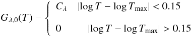 (4)and require
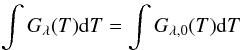 (5)so that
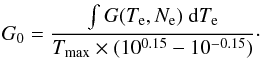 (6)The values of the constant Cλ are calculated using the CHIANTI routine integral_calc. The estimate for the emission measure at the temperature of a single line, EMjw, is then simply obtained from the observed intensity Io:
 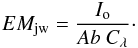 (7)The points are normally close to the minima of the EM loci curves, if the emission lines are not blended. The minima of the EM loci curves (Io/Gλ(T)) are by definition upper limits to the EM distribution, which however can be very different (see Del Zanna 1999; Del Zanna et al. 2002 for details).
Spectral lines used for the DEM inversion.
We used CHIANTI v.7.1 (Landi et al. 2013) atomic data and ionisation equilibrium tables. We use the new set of abundances for the 3 MK loops obtained by Del Zanna (2013b) and Del Zanna & Mason (2014). We note that these abundances present a first ionisation potential (FIP) enhancement of about a factor of 3.2, slightly lower than the factor of 4 of the Feldman (1992) coronal abundances. The fact that active region cores are better represented by coronal abundances was already pointed out by Tripathi et al. (2011). However, we point out that our DEM results between 1 and 3 MK are entirely independent of elemental abundance issues, since they are based only on iron lines. The list of the spectral lines used for DEM analysis is given in Table 1. They are mostly from iron, although a few low FIP elements were also used to constrain lower and higher temperatures (outside the range 1–3 MK).
4. Results
4.1. Spatial variability
 |
Fig. 4 The slopes of the EM distribution in the 1–3 MK temperature range, as estimated from the AIA DEM, the approximate Pottasch method applied to the AIA data, the EIS DEM, and the Pottasch method applied to the EIS observations. The AIA slopes are obtained from full-resolution (1′′) images averaged over 13:30–13:31 UT. The top row shows the images of the slopes, the middle the profiles along the vertical line shown in the images, and the bottom row the histograms of the distribution of the slopes. |
One natural question we wanted to address is the amount of spatial variability within an AR. Another issue that we wanted to address is whether the lower spatial resolution of EIS had any influence on the result. The higher-resolution AIA images clearly show a lot more loop structures within the cores of ARs, so in principle we could expect higher slopes. Another question is how much the results depend on the different methods. We compare the results of four methods in Fig. 4.
First, we obtained a DEM for each AIA pixel using a faster version of the regularised inversion method described by Hannah & Kontar (2012). We used as kernel the AIA responses that we calculated using CHIANTI v.7.1 (Landi et al. 2013), and the Del Zanna (2013b) AR core abundances. We then fitted a line in the log T −log EM plot in the 1–3 MK range, and obtained the slopes shown in Fig. 4 (first column from the left). The slopes, over the whole of the AR core, range between 2 and 5, with the most frequent value around 3.5.
Second, we have considered a faster method (similar to the Pottasch 1963 one) applied to the AIA data. We have considered the intensity of the 171 Å band as only being due to Fe IX, and used the AIA 171 Å response function instead of the G(T) to estimate the EM at 1 MK. To estimate the EM at 3 MK, we have calculated the AIA 335 Å response function by including only the emissivity of the Fe XVI 335 Å line, and estimated the observed AIA DN/s due to Fe XVI 335 Å following the method developed by Del Zanna (2013b). The estimate of the EM slope in the 1–3 MK range obtained from AIA is shown in Fig. 4 (second column from the left). There is much less variation in the slopes, but the most frequent value is around 3.5.
Third, we obtained the slopes applying the XRT_DEM_ITERATIVE2 method to the EIS intensities to obtain the DEM. We then calculated the EM(0.1) values, and fitted them in the 1–3 MK range to obtain the slopes shown in Fig. 4 (third column from the left). The slopes are slightly higher, with the most frequent value around 4.
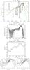 |
Fig. 6 From top to bottom: 1) DEM for the 19 Apr. AR core, obtained with the spline method (black smooth curve), with the MCMC_DEM program (red curve) and XRT_DEM method (green curve). The points are plotted at their effective temperature, and the values in brackets indicate the ratio between predicted and observed intensity. 2) The results of the Monte Carlo XRT_DEM inversion. 3) The DEM obtained from MCMC_DEM. 4) The EM(0.1) values obtained from the DEM, together with the curves for the EM loci, and the slopes (dashed lines). The EMjw points (triangles) are also shown, with their slopes (dot-dash lines). The left bottom plot is with the new Hinode EIS calibration (slope = 4.4 from the EM(0.1) and 3.8 from the EMjw points), the right one with the ground calibration (slope = 3.6 from the EM(0.1) and 3.3 from the EMjw points). |
Finally, we computed the EMjw values for two EIS lines emitted near 1 (Fe ix 188.5 Å) and 3 MK (Fe xvi 263.0 Å) and obtained the slope by fitting a straight line. The last column in Fig. 4 shows the slope obtained in this way. We can see that as in the AIA case, the slopes in the core of the active region have less variability and are slightly lower, around 3.
We performed the same analysis on the second rotation. The results are shown in Fig. 5. The slopes in the areas where the Fe xvi emission is low are masked out (in blue) in Figs. 4, 5. They correspond to areas where the DN/s in the Fe xvi 263.0 Å line were below 60, and where the estimated DN/s due to the Fe xvi 335 Å line in the AIA 335 Å channel were below 20.
4.2. DEM of the AR core for the first rotation
As shown in Fig. 2 (dashed lines), we selected a region within the AR core for a detailed DEM analysis. We averaged the EIS spectra and obtained calibrated radiances. We measured the electron density using ratios from Fe XIII (202.0 vs. 203.8 Å) and Fe XIV (264.7 vs. 270.5 Å). For both ions, we obtained a density in the core region of 4 × 109 cm-3. We used this value to calculate the line emissivities for the DEM inversion, although we note that the choice of density has little effect on the line emissivities, because of the choice of lines.
The results of the three DEM inversions methods are shown in the top panel of Fig. 6. We obtain a distribution with a well-defined peak at 3 MK, and very good agreement (to within 20–30%) between observed and predicted intensities. There is good agreement between the three different DEM inversions methods in the 1–3 MK region, which is reassuring.
The MCMC_DEM program was run with a temperature grid of log T[K] = 0.1. It tends to underestimate the peak of the DEM at 3 MK, while the emission measure above 3 MK is overestimated. If a finer grid is chosen, the DEM peak tends to agree with the spline method, but the DEM in the 1–3 MK range shows large deviations (for a discussion on the MCMC_DEM grid size see Landi et al. 2012; Testa et al. 2012). The XRT_DEM method was run on a finer grid, log T[K] = 0.05, which produces good agreement with the spline method at the peak.
The middle panels of Fig. 6 display the results of the Monte Carlo XRT_DEM and MCMC_DEM inversions. The XRT_DEM simulations are obtained by randomly varying (400 times) the input intensities within the estimated uncertainties, which have been taken as 20%, the overall uncertainty in the EIS calibration (Del Zanna 2013a), added to the uncertainty from the fitting. The ‘error bars’ on the MCMC_DEM plots are obtained using the default values originating from the iterative runs of the program. The Monte Carlo simulations suggest an uncertainty of about 0.4 dex on the EM slopes.
The bottom (left) panel of Fig. 6 displays the EM(0.1) values obtained from the spline DEM, together with the curves for the EM loci. The dashed line indicates a slope of 4.4 for the EM between 1–3 MK. We note that if the EMjw points are considered, the slope becomes 3.8, in agreement with what obtained from just the two Fe IX 188.5 Å and the Fe XVI 263.0 Å lines, shown in Fig. 2). In other words, the EM approximation tends to under-estimate the slope. This can be understood by the fact that the Jordan & Wilson (1971) approximation is close to the loci of the EM loci curves, which are upper limits to the EM(0.1) values.
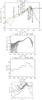 |
Fig. 7 Same as Fig. 6, for the 17 May 2011 second rotation. The dashed line in the bottom plot indicates a slope of 4.6 from the EM(0.1), while the dot-dash line a slope of 3.9 from the EMjw points. |
We note that Del Zanna (2013a) has shown that the intensities of all the strong EIS lines formed in the 2–3 MK range (in the long-wavelength channel) have been underestimated by about a factor of two, for data taken after 2009, hence most previous analyses have underestimated the slope of the EM in the 1–3 MK range. This is because all the strong EIS lines formed around 1 MK are in the EIS short-wavelength channel, which has not been affected so much by degradation. Figure 6 (bottom right) shows the EM results obtained form the same data, but adopting the ground calibration. The EMjw slope is 3.3 (ground calibration) instead of 3.8, while the slope obtained from the EM(0.1) values is 3.6 instead of 4.4.
4.3. DEM of the AR core for the second rotation
As shown in Fig. 3 (dashed lines), we selected a region within the AR core for a detailed DEM analysis. We measured the electron density using ratios from Fe XIII (202.0 vs. 203.8 Å) and Fe XIV (264.7 vs. 270.5 Å). For both ions, we obtained a density in the core region of 2 × 109 cm-3. The density has decreased by a factor of 2 in comparison to the first rotation. We used this value to calculate the line emissivities for the DEM inversion.
The DEM and EM results are shown in Fig. 7. Again, there is good agreement among the inversion methods. The slope from the EM(0.1) values is 4.6, while that from the EMjw points is lower, 3.9, as we have seen previously. We recall that any background subtraction would significantly lower the 1 MK emission, increasing the EM slope.
5. Summary and conclusions
In the present paper, we have studied the EM distribution in the core of active region NOAA 11193, once when it appeared for the first time near the central meridian on the visible solar disk (when it was 9 days old) and again when it appeared near the central meridian after a solar rotation. Our analysis shows that there is significantly higher emission measure at high temperature in the active region core when the active region is younger. The density decreases by a factor of two between the two rotations.
The slope of EM distribution between 1–3 MK, measured using various methods ranged between 2 and 5 throughout the core of the active region during the first rotation, with values around 4–5 in the hottest regions. In a carefully chosen region inside the core by avoiding any possible contamination from bright moss regions we find a slope of the EM curve to be 4.4 ± 0.4.
During the second rotation of the active region, the slope between 1–3 MK, measured using various methods also ranged between 2 to 5, although in most of the core regions lower values are present. We find that despite the overall reduction in the EM at high temperatures, the slope of the EM between 1 and 3 MK in the hottest regions (where Fe XVI is strongest) appears to change little. In fact, a carefully selected region without contamination from bright moss shows a slope of 4.6 ± 0.4, i.e. similar to that of the previous rotation.
Additionally, we have also studied which factors affect the measurement of the slope of the EM distribution between 1 MK and 3 MK obtained from Hinode EIS measurements. The revised EIS calibration has an important effect, by raising the slopes by about 0.8. The Jordan & Wilson approximate method consistently underestimates the slope by about 0.5. We have indeed carried out the analysis of one of the regions selected in Tripathi et al. (2011) and found a similar underestimation. We have tested different inversion methods and have found consistent DEM distributions within the 1–3 MK range.
To the best our knowledge, using AIA and EIS observations for the first time we have shown that the slopes significantly vary within the cores of an AR, by about ±1 in the hottest regions. There are some slight differences between the slopes obtained with Hinode/EIS and SDO/AIA. These are partly due to the better spatial resolution of SDO/AIA. Approximate methods tend to underestimate the slopes, compared to those based on the full DEM inversion. We therefore suggest that future studies obtain the EM slopes after performing a full DEM inversion.
We also pointed out the need to carefully select representative regions, using the much higher AIA spatial resolution, to avoid areas where significant line-of-sight (mostly background) emission is present. This is often almost impossible to achieve at the EIS resolution. During the second rotation, line-of-sight contamination at 1 MK is more significant than during the first rotation. The slopes we provide are without background subtraction. Taking the background subtraction into account would increase the slope of the EM, especially for the second rotation. In any case, the slopes in the range 4–5 found for NOAA 11193 are consistent with high frequency heating occurring during the evolution of the active region.
We believe that this study provides an important contribution to the problem of coronal heating in active region cores, in particular by exploring in depth the uncertainties in such analyses.
Acknowledgments
G.D.Z., H.E.M. and B.O.D. acknowledge support from STFC. BOD also acknowledges support from the Gates Cambridge Trust and Inter-University Centre for Astronomy and Astrophysics (IUCAA) for the hospitality during his visit. This work has benefited from discussions at a series of ISSI workshops. Hinode is a Japanese mission developed and launched by ISAS/JAXA, with NAOJ as domestic partner and NASA and STFC (UK) as international partners. It is operated by these agencies in co-operation with ESA and NSC (Norway). We acknowledge the use of the SDO/AIA observations for this study. The data are provided courtesy of NASA/SDO, LMSAL, and the AIA, EVE, and HMI science teams. CHIANTI is a collaborative project involving George Mason University, the University of Michigan (USA) and the University of Cambridge (UK). We would like to thank Amy Winebarger for useful comments on the manuscript.
References
- Bradshaw, S. J., Klimchuk, J. A., & Reep, J. W. 2012, ApJ, 758, 53 [NASA ADS] [CrossRef] [Google Scholar]
- Cargill, P. J. 2014, ApJ, 784, 49 [NASA ADS] [CrossRef] [Google Scholar]
- Craig, I. J. D., & Brown, J. C. 1976, A&A, 49, 239 [NASA ADS] [Google Scholar]
- Craig, I. J. D., & Brown, J. C. 1986, Inverse problems in astronomy: A guide to inversion strategies for remotely sensed data, Adam Hilger, Ltd., 159 [Google Scholar]
- Culhane, J. L., Harra, L. K., James, A. M., et al. 2007, Sol. Phys., 243, 19 [Google Scholar]
- Dadashi, N., Teriaca, L., Tripathi, D., Solanki, S. K., & Wiegelmann, T. 2012, A&A, 548, A115 [NASA ADS] [CrossRef] [EDP Sciences] [Google Scholar]
- Del Zanna, G. 1999, Ph.D. Thesis, Univ. of Central Lancashire, UK [Google Scholar]
- Del Zanna, G. 2013a, A&A, 555, A47 [NASA ADS] [CrossRef] [EDP Sciences] [Google Scholar]
- Del Zanna, G. 2013b, A&A, 558, A73 [NASA ADS] [CrossRef] [EDP Sciences] [Google Scholar]
- Del Zanna, G., & Mason, H. E. 2003, A&A, 406, 1089 [NASA ADS] [CrossRef] [EDP Sciences] [Google Scholar]
- Del Zanna, G., & Mason, H. E. 2014, A&A, 565, A14 [NASA ADS] [CrossRef] [EDP Sciences] [Google Scholar]
- Del Zanna, G., Landini, M., & Mason, H. E. 2002, A&A, 385, 968 [NASA ADS] [CrossRef] [EDP Sciences] [Google Scholar]
- Del Zanna, G., O’Dwyer, B., & Mason, H. E. 2011, A&A, 535, A46 [NASA ADS] [CrossRef] [EDP Sciences] [Google Scholar]
- Delaboudinière, J.-P., Artzner, G. E., Brunaud, J., et al. 1995, Sol. Phys., 162, 291 [NASA ADS] [CrossRef] [Google Scholar]
- Feldman, U. 1992, Phys. Scr, 46, 202 [NASA ADS] [CrossRef] [Google Scholar]
- Guennou, C., Auchère, F., Klimchuk, J. A., Bocchialini, K., & Parenti, S. 2013, ApJ, 774, 31 [NASA ADS] [CrossRef] [Google Scholar]
- Handy, B. N., Acton, L. W., Kankelborg, C. C., et al. 1999, Sol. Phys., 187, 229 [NASA ADS] [CrossRef] [Google Scholar]
- Hannah, I. G., & Kontar, E. P. 2012, A&A, 539, A146 [NASA ADS] [CrossRef] [EDP Sciences] [Google Scholar]
- Jordan, C., & Wilson, R. 1971, Physics of the Solar Corona, Proc. Nato Adv. Study Inst. (Dordrecht: Reidel), 27, 219 [Google Scholar]
- Judge, P. G., Hubeny, V., & Brown, J. C. 1997, ApJ, 475, 275 [NASA ADS] [CrossRef] [EDP Sciences] [Google Scholar]
- Kashyap, V., & Drake, J. J. 1998, ApJ, 503, 450 [NASA ADS] [CrossRef] [Google Scholar]
- Klimchuk, J. A. 2006, Sol. Phys., 234, 41 [NASA ADS] [CrossRef] [Google Scholar]
- Klimchuk, J. A. 2009, in The Second Hinode Science Meeting: Beyond Discovery-Toward Understanding, eds. B. Lites, M. Cheung, T. Magara, J. Mariska, & K. Reeves, ASP Conf. Ser., 415, 221 [Google Scholar]
- Landi, E., Reale, F., & Testa, P. 2012, A&A, 538, A111 [NASA ADS] [CrossRef] [EDP Sciences] [Google Scholar]
- Landi, E., Young, P. R., Dere, K. P., Del Zanna, G., & Mason, H. E. 2013, ApJ, 763, 86 [NASA ADS] [CrossRef] [Google Scholar]
- Lemen, J. R., Title, A. M., Akin, D. J., et al. 2012, Sol. Phys., 275, 17 [NASA ADS] [CrossRef] [Google Scholar]
- Mulu-Moore, F. M., Winebarger, A. R., & Warren, H. P. 2011, ApJ, 742, L6 [NASA ADS] [CrossRef] [Google Scholar]
- O’Dwyer, B., Del Zanna, G., Mason, H. E., Weber, M. A., & Tripathi, D. 2010, A&A, 521, A21 [NASA ADS] [CrossRef] [EDP Sciences] [Google Scholar]
- O’Dwyer, B., Del Zanna, G., & Mason, H. E. 2014, A&A, 561, A20 [NASA ADS] [CrossRef] [EDP Sciences] [Google Scholar]
- Poduval, B., DeForest, C. E., Schmelz, J. T., & Pathak, S. 2013, ApJ, 765, 144 [NASA ADS] [CrossRef] [Google Scholar]
- Pottasch, S. R. 1963, ApJ, 137, 945 [NASA ADS] [CrossRef] [Google Scholar]
- Schmelz, J. T., & Pathak, S. 2012, ApJ, 756, 126 [NASA ADS] [CrossRef] [Google Scholar]
- Sheeley, N. R. 1981, in Solar Active regions (Colorado Associated University Press), 17 [Google Scholar]
- Subramanian, S., Tripathi, D., Klimchuk, J. A., & Mason, H. E. 2014, ApJ, 795, 76 [NASA ADS] [CrossRef] [Google Scholar]
- Testa, P., De Pontieu, B., Martínez-Sykora, J., Hansteen, V., & Carlsson, M. 2012, ApJ, 758, 54 [NASA ADS] [CrossRef] [Google Scholar]
- Tripathi, D., Mason, H. E., Dwivedi, B. N., del Zanna, G., & Young, P. R. 2009, ApJ, 694, 1256 [NASA ADS] [CrossRef] [Google Scholar]
- Tripathi, D., Mason, H. E., Del Zanna, G., & Young, P. R. 2010a, A&A, 518, A42 [NASA ADS] [CrossRef] [EDP Sciences] [Google Scholar]
- Tripathi, D., Mason, H. E., & Klimchuk, J. A. 2010b, ApJ, 723, 713 [NASA ADS] [CrossRef] [Google Scholar]
- Tripathi, D., Klimchuk, J. A., & Mason, H. E. 2011, ApJ, 740, 111 [NASA ADS] [CrossRef] [Google Scholar]
- Tripathi, D., Mason, H. E., & Klimchuk, J. A. 2012, ApJ, 753, 37 [NASA ADS] [CrossRef] [Google Scholar]
- Ugarte-Urra, I., & Warren, H. P. 2012, ApJ, 761, 21 [NASA ADS] [CrossRef] [Google Scholar]
- Ugarte-Urra, I., Warren, H. P., & Brooks, D. H. 2009, ApJ, 695, 642 [NASA ADS] [CrossRef] [Google Scholar]
- Viall, N. M., & Klimchuk, J. A. 2011, ApJ, 738, 24 [Google Scholar]
- Viall, N. M., & Klimchuk, J. A. 2012, ApJ, 753, 35 [NASA ADS] [CrossRef] [Google Scholar]
- Warren, H. P., Winebarger, A. R., & Mariska, J. T. 2003, ApJ, 593, 1174 [NASA ADS] [CrossRef] [Google Scholar]
- Warren, H. P., Ugarte-Urra, I., Doschek, G. A., Brooks, D. H., & Williams, D. R. 2008, ApJ, 686, L131 [NASA ADS] [CrossRef] [Google Scholar]
- Warren, H. P., Winebarger, A. R., & Brooks, D. H. 2010, ApJ, 711, 228 [NASA ADS] [CrossRef] [Google Scholar]
- Warren, H. P., Brooks, D. H., & Winebarger, A. R. 2011, ApJ, 734, 90 [NASA ADS] [CrossRef] [Google Scholar]
- Warren, H. P., Winebarger, A. R., & Brooks, D. H. 2012, ApJ, 759, 141 [NASA ADS] [CrossRef] [Google Scholar]
- Weber, M. A., Deluca, E. E., Golub, L., & Sette, A. L. 2004, in Multi-Wavelength Investigations of Solar Activity, eds. A. V. Stepanov, E. E. Benevolenskaya, & A. G. Kosovichev, IAU Symp., 223, 321 [Google Scholar]
- Winebarger, A. R., Warren, H. P., & Seaton, D. B. 2003, ApJ, 593, 1164 [NASA ADS] [CrossRef] [Google Scholar]
- Winebarger, A. R., Schmelz, J. T., Warren, H. P., Saar, S. H., & Kashyap, V. L. 2011, ApJ, 740, 2 [NASA ADS] [CrossRef] [Google Scholar]
- Winebarger, A., Tripathi, D., Mason, H. E., & Del Zanna, G. 2013, ApJ, 767, 107 [NASA ADS] [CrossRef] [Google Scholar]
All Tables
All Figures
|
Fig. 1 AIA negative images of active region NOAA 11193 when it first appeared on the visible solar disk near the central meridian on Apr. 19, 2011 (left) and during the second rotation on May 17, 2011 (right). The intensities are DN/s, and the images of the two dates are shown on the same intensity scale and field of view. Coordinates are arcseconds from Sun centre. |
| In the text | |
|
Fig. 2 AIA (DN/s, first and second row) and EIS (radiances in phot cm-2 st-1 s-1, third and fourth row) negative images on Apr. 19, 2011. The arrows indicate the AR core region selected for DEM analysis. The bottom plots show the profiles of the intensities along this vertical line. The dashed vertical lines in the bottom plots indicate the region selected for DEM analysis. |
| In the text | |
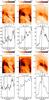 |
Fig. 3 Same as Fig. 2, for the 17 May 2011 second rotation. |
| In the text | |
|
Fig. 4 The slopes of the EM distribution in the 1–3 MK temperature range, as estimated from the AIA DEM, the approximate Pottasch method applied to the AIA data, the EIS DEM, and the Pottasch method applied to the EIS observations. The AIA slopes are obtained from full-resolution (1′′) images averaged over 13:30–13:31 UT. The top row shows the images of the slopes, the middle the profiles along the vertical line shown in the images, and the bottom row the histograms of the distribution of the slopes. |
| In the text | |
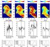 |
Fig. 5 Same as Fig. 4, for the second rotation. |
| In the text | |
|
Fig. 6 From top to bottom: 1) DEM for the 19 Apr. AR core, obtained with the spline method (black smooth curve), with the MCMC_DEM program (red curve) and XRT_DEM method (green curve). The points are plotted at their effective temperature, and the values in brackets indicate the ratio between predicted and observed intensity. 2) The results of the Monte Carlo XRT_DEM inversion. 3) The DEM obtained from MCMC_DEM. 4) The EM(0.1) values obtained from the DEM, together with the curves for the EM loci, and the slopes (dashed lines). The EMjw points (triangles) are also shown, with their slopes (dot-dash lines). The left bottom plot is with the new Hinode EIS calibration (slope = 4.4 from the EM(0.1) and 3.8 from the EMjw points), the right one with the ground calibration (slope = 3.6 from the EM(0.1) and 3.3 from the EMjw points). |
| In the text | |
|
Fig. 7 Same as Fig. 6, for the 17 May 2011 second rotation. The dashed line in the bottom plot indicates a slope of 4.6 from the EM(0.1), while the dot-dash line a slope of 3.9 from the EMjw points. |
| In the text | |
Current usage metrics show cumulative count of Article Views (full-text article views including HTML views, PDF and ePub downloads, according to the available data) and Abstracts Views on Vision4Press platform.
Data correspond to usage on the plateform after 2015. The current usage metrics is available 48-96 hours after online publication and is updated daily on week days.
Initial download of the metrics may take a while.