| Issue |
A&A
Volume 573, January 2015
|
|
|---|---|---|
| Article Number | A121 | |
| Number of page(s) | 11 | |
| Section | The Sun | |
| DOI | https://doi.org/10.1051/0004-6361/201424029 | |
| Published online | 09 January 2015 | |
Scattering polarization of Mg I b triplet in solar chromosphere
1
Yunnan Observatories, Chinese Academy of Sciences,
Kunming, Yunnan
650011, PR
China
e-mail: sayahoro@ynao.ac.cn
2
Graduate School of University of Chinese Academy of
Sciences, Yuquan
Road, Shijingshang Block
Beijing
100049, PR
China
Received:
18
April
2014
Accepted:
12
November
2014
Aims. The magnetic field in the chromosphere of the quiet sun is too weak to be diagnosed via the general Zeeman effect. To obtain the hidden magnetic field vector, a complete comprehension of the linear polarization produced by scattering and modified by magnetic field is needed. We report a systematic and quantitative investigation of the sensitivity of the fractional linear polarization of the magnesium triplet to a weak magnetic field in the chromosphere, which can be a guide for the diagnostics of a weak magnetic field in the solar chromosphere.
Methods. We focus on the fractional linear polarization of the magnesium triplet induced by scattering. We use the quantum theory under the flat-spectrum approximation developed by Landi Degl’Innocenti for the investigation. A seven-level atomic model of magnesium is adopted, while we do not take the radiative transfer or partial frequency redistribution (PRD) into account.
Results. Polarization is directly related to the anisotropy factor, and modified by the continuum, collision, and magnetic field as well as dichroism effect. In our calculation, the elastic collision rates found are not large enough to destroy the population imbalances of the lower levels of the b2 and b1 lines. This is the prerequisite for the lower level Hanle effect and dichroism effect. When considering the dichroism effect, the magnetic field can influence the polarization not only in the line cores but also in the line wings. However, the magnetic field cannot obviously influence the polarization degree in the line wings once the continuum becomes significant. The polarization of the triplet is sensitive to the magnetic field between 0.001 and 0.1 Gauss due to the lower level Hanle effect and between 1 and 10 Gauss due to the upper level Hanle effect. In the lower level Hanle effect dominated region, the Q/I amplitude of the b4 line increases with magnetic field strength because of the coupling among atomic alignments of the involved levels as described in the statistical equilibrium equations, while the amplitudes of the b2 and b1 lines decrease. In the upper level Hanle effect dominated region, the most sensitive line is the b4.
Conclusions. The polarized lower levels and the contribution of dichroism have to be considered to fit the observed profiles of Mg I b triplet in the line cores. Therefore the b2 and b1 lines can be potential candidates for probing sub-Gauss range magnetic field, because their Q/I amplitudes are sensitive to the magnetic field strength between 0.001 and 0.1 Gauss due to the lower level Hanle effect. The b4 line is suitable for diagnostics of magnetic field between 1 Gauss and 10 Gauss.
Key words: polarization / Sun: chromosphere / magnetic fields / line: profiles / atomic processes
© ESO, 2015
1. Introduction
Solar chromosphere is a passage where the matter and energy transport from the photosphere to the corona. The magnetic field in the chromosphere outside the active region is usually weaker than 100 Gauss (Trujillo Bueno et al. 2004). Measuring the chromospheric magnetic field vector is strongly desired for understanding essential structures, and energy storage and release for solar eruptions, but it is notoriously difficult and challenging. It is well known that the measurement is feasible via the Zeeman effect for probing a relatively strong magnetic field, and via the Hanle effect for detecting weak magnetic field (see reviews by, e.g., Stenflo 2003; Trujillo Bueno 2003). In fact, diagnosing a weak magnetic field through the Hanle effect is also a very complicated mission and it needs a complete physical comprehension of the polarization and depolarization mechanisms.
As pointed out by Stenflo (2013), the second solar spectrum, originated from the scattering processes close to the solar disk limb, is a playground for the Hanle effect through which one can reveal various types of physical effects like J state interference, continuum polarization, optical pumping, hyperfine structure, and isotope effects. Observation with sensitivities of an order of 10-4–10-5 have shown some great details of the spectral richness and complexity of the second solar spectrum (Stenflo 1996; Stenflo & Keller 1997), and Gandorfer (2000, 2002, 2005) also compiled serial Atlas of the second solar spectrum from the deep UV to the near infrared. It reveals that the linear polarization signal is mainly produced by the population imbalances of the atomic levels, which is caused by the anisotropic incident radiation through the optical pumping. This is the so-called atomic polarization, and often refers to resonance lines. More importantly, a magnetic field can modify this population imbalance via the Hanle effect and can produce an observable signal. It is believed that in this way the magnetic vector can be diagnosed.
As is well known, the fractional polarization profiles will be significantly changed when
the magnetic field strength B locates  (1)with
  (2)where tlife and
gJ are the lifetime (in
seconds) of upper or lower level and the Landé
factor of the J
level under consideration, respectively, and Bc indicates the critical magnetic field
strength.
(2)where tlife and
gJ are the lifetime (in
seconds) of upper or lower level and the Landé
factor of the J
level under consideration, respectively, and Bc indicates the critical magnetic field
strength.
We focus on the scattering induced linear polarization and the Hanle effect of Mg I b lines with polarized lower levels. The three lines (b4 5168.761 Å, b2 5174.125 Å, and b1 5185.048 Å) share the same upper level, 3S1, and sit on three different metastable lower levels, 3P0,1,2 (Kelleher & Podobedova 2008). They are formed in the lower layers of the chromosphere and some of them are proven to be suitable to diagnose the magnetic field in the chromosphere via the Zeeman effect (Lites et al. 1988). However, identifying their suitability to probe the weak magnetic field is the task of this work. Observation of Mg I b triplet close to the solar limb by Stenflo et al. (2000) shows similar Q/I amplitudes. To explain the observation, we need to consider the polarizations of the lower levels and the dichroism contribution (see Trujillo Bueno 1999, 2001, 2009). From Eqs. (1) and (2) along with the values of tlife and gu, one can find that the linear polarizations of these lines are very sensitive to the sub-Gauss magnetic field due to the lower level Hanle effect, and to the Gauss magnetic field due to the upper level Hanle effect. Therefore it satisfies the basic requirement as a useful tool to diagnose the weak chromosphere magnetic field like Ca II IR triplet (Manso Sainz & Trujillo Bueno 2010). Based on previous studies, our main target is to study how the fractional linear polarization Q/I and U/I profiles of Mg I b triplet behave with a weak magnetic field and how other mechanisms influence the polarization. We use the quantum theory proposed by Bommier (1980) and developed by Landi Degl’Innocenti (1983, 1984) under the flat-spectrum approximation using a slab scattering model.
The outline of this paper is as follows. In Sect. 2, we briefly skip the theoretical framework of the statistical equilibrium equations in the density matrix formalism. The roles of the anisotropic incident radiation, continuum, and collision in modifying the polarizations of the lower levels are presented in Sect. 3. In Sect. 4, the lower level Hanle effect in both line cores and line wings of the triplet is studied quantitatively. Finally, our main conclusions are summarized in the last section.
2. Models and formulations
In this section, we first describe the atomic model of the neutral magnesium, and then a simplified scattering model used in this paper, as well as the associated statistical equilibrium equations of the density matrix formalism. All of these form the theoretical basis of our calculations.
2.1. The atomic model
We adopt a seven-level atomic model of neutral 24Mg atom, which consists of the upper levels 3S4P 3P0,1,2, the middle level 3S4S 3S1 (i.e., the upper level of the Mg I b triplet), and metastable lower levels 3S3P 3P0,1,2. Because of the fact that 24Mg does not have net nuclear spin, we did not take the hyperfine structure into account while a total of six electric dipole transitions are under consideration. The transition probabilities of magnesium given by Kelleher & Podobedova (2008) are listed in Table 1 and compiled at National Institute of Standards and Technology (NIST) atomic spectra database (Kramida et al. 2013). The Landé factors are calculated under LS coupling approximation.
Data for seven-level atomic model of Mg I.
2.2. The scattering model
For simplicity, a plane parallel slab model is adopted, where the atmosphere is
simplified to be an optically thin slab and composed of magnesium atoms, thus the
radiative transfer is not considered. This model was also used by Manso Sainz & Landi Degl’Innocenti (2002) and Belluzzi et al. (2007, 2009) to investigate the theoretical profiles of the second solar spectrum. A
reference system with z axis directed along the solar radius is adopted,
and the radiation field is described by means of the irreducible tensor of the radiation
(Landi Degl’Innocenti 1983),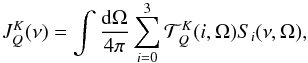 (3)where
Si(ν,Ω) =
I,Q,U,V indicate the four Stokes parameters, and
(3)where
Si(ν,Ω) =
I,Q,U,V indicate the four Stokes parameters, and
 is the irreducible spherical
tensor to signify the geometry of the incident radiation. Assuming that the incident
radiation field is unpolarized and axissymmetric about the radius, it is easily understood
that only two components
is the irreducible spherical
tensor to signify the geometry of the incident radiation. Assuming that the incident
radiation field is unpolarized and axissymmetric about the radius, it is easily understood
that only two components  and
and
 are nonzero in this system,
![\begin{eqnarray} \label{eq:4} J^0_0(\nu)&=&\oint\frac{{\rm d}\Omega}{4\pi}I(\nu,\mu), \nonumber \\ J^2_0(\nu)&=&\oint\frac{{\rm d}\Omega}{4\pi}\left[\frac{1}{2\sqrt{2}}\left(3\mu^2-1\right)I(\nu,\mu)\right], \end{eqnarray}](/articles/aa/full_html/2015/01/aa24029-14/aa24029-14-eq40.png) (4)where
I(ν,μ) is the incident radiation
intensity, and μ =
cosθ with θ indicating the heliocentric angle. Note that
is the mean radiation
intensity, and the atomic polarization comes from due to the anisotropy of the
radiation intensity. For simplicity, we use two dimensionless quantities
(4)where
I(ν,μ) is the incident radiation
intensity, and μ =
cosθ with θ indicating the heliocentric angle. Note that
is the mean radiation
intensity, and the atomic polarization comes from due to the anisotropy of the
radiation intensity. For simplicity, we use two dimensionless quantities
 ,
the mean number of photons, and then wν, the anisotropy
factor describing the incident radiation field. The values of
and wν are related to the
radiation field tensor components through the equations,
,
the mean number of photons, and then wν, the anisotropy
factor describing the incident radiation field. The values of
and wν are related to the
radiation field tensor components through the equations,  (5)The mean number
of photons can be estimated by
(5)The mean number
of photons can be estimated by  (6)In the following,
we adopt a typical temperature T = 5755 K from the FLA-C atmosphere model (Fontenla et al. 1993) at a height of 905 km, a mean
formation height where the magnesium triplet is roughly considered to be formed. We do not
consider the quantum interferences between different J levels in our
calculation, because the value of
(6)In the following,
we adopt a typical temperature T = 5755 K from the FLA-C atmosphere model (Fontenla et al. 1993) at a height of 905 km, a mean
formation height where the magnesium triplet is roughly considered to be formed. We do not
consider the quantum interferences between different J levels in our
calculation, because the value of  is too small to influence the scattering polarization profile in the typical solar
situation (Belluzzi & Trujillo Bueno 2011).
is too small to influence the scattering polarization profile in the typical solar
situation (Belluzzi & Trujillo Bueno 2011).
2.3. The statistical equilibrium equations
The density matrix was introduced by Fano (1957) to
describe the excitation states of the atomic system. The diagonal matrix elements are the
population of the atomic levels, and the nondiagonal matrix elements are the interference
term. Here, we adopt the multipolar components of the atom density matrix (Omont 1977; Landi
Degl’Innocenti 1996):  (7)where
K = 0, 1,
..., 2J,
Q = −K, −
K + 1, ..., K − 1, K. The expression in
brackets is the Wigner 3j symbol, and
(7)where
K = 0, 1,
..., 2J,
Q = −K, −
K + 1, ..., K − 1, K. The expression in
brackets is the Wigner 3j symbol, and  indicates the total
population of the level. In the situation of weak anisotropy of the radiation field
(corresponding to the condition of the solar chromosphere), the tensor of rank 1 indicates
the orientation components contributing to the circular polarization and the tensor of
rank 2 signifies the alignment components contributing to the linear polarization, while
the tensor of rank K larger than 2 is too weak to influence the line
profile.
indicates the total
population of the level. In the situation of weak anisotropy of the radiation field
(corresponding to the condition of the solar chromosphere), the tensor of rank 1 indicates
the orientation components contributing to the circular polarization and the tensor of
rank 2 signifies the alignment components contributing to the linear polarization, while
the tensor of rank K larger than 2 is too weak to influence the line
profile.
The statistical equilibrium equations without quantum interference between the sublevels
pertaining to different J levels were derived by Landi Degl’Innocenti & Landolfi (2004). The equations are valid
under the flat-spectrum approximation. In contrast to the partial frequency redistribution
(PRD), this approximation is also called the complete frequency redistribution (CRD). It
is noteworthy that the PRD theory (Bommier
1997a,b) causes significantly different
results from the CRD theory, but PRD theory becomes dominant only for a limited number of
very strong lines (e.g., Ca II, Mg II resonance lines, Ly-alpha), mainly in the line
wings. So the CRD theory is still a robust approach to investigate the Mg I b triplet. On
the other hand, the collision rates scale can simply be added to the corresponding
radiative rates in the statistical equilibrium equation under the impact approximation,
which requires that the collision time is much smaller than the relaxation time scale due
to radiative rates: ![\begin{eqnarray} \label{eq:8} \frac{{\rm d}}{{\rm d}t}\rho_Q^K(\alpha J)&=&-2\pi {\rm i}\nu_{\rm L}g_{\alpha J}Q\rho_Q^K(\alpha J)\nonumber \\ &&+~\sum\limits_{\alpha_\ell J_\ell}\sum\limits_{K_\ell Q_\ell }\rho_{Q_\ell}^{K_\ell}(\alpha_\ell J_\ell)\mathbb{T}_{\rm A}(\alpha JKQ,\alpha_\ell J_\ell K_\ell Q_\ell) \nonumber \\ &&+~\sum\limits_{\alpha_u J_u}\sum\limits_{K_u Q_u}\rho_{Q_u}^{K_u}(\alpha_u J_u)[\mathbb{T}_{\rm E}(\alpha JKQ,\alpha_u J_u K_u Q_u) \nonumber \\ &&+~\mathbb{T}_{\rm S}(\alpha JKQ,\alpha_u J_u K_u Q_u)] \nonumber \\ &&-\!\!\sum\limits_{K'Q'}\rho_{Q'}^{K'}(\alpha J)\bigg[\mathbb{R}_{\rm A}(\alpha JKQK'Q')+\mathbb{R}_{\rm E}(\alpha JKQK'Q') \nonumber \\ &&+~\mathbb{R}_{\rm S}(\alpha JKQK'Q')\bigg] \nonumber \\ &&+~\sum\limits_{\alpha_\ell J_\ell}\sqrt{\frac{2J_\ell+1}{2J+1}}C_{\rm I}^{(K)}(\alpha J,\alpha_\ell J_\ell)\rho_Q^K(\alpha_\ell J_\ell) \nonumber \\ &&+~\sum\limits_{\alpha_u J_u}\sqrt{\frac{2J_u+1}{2J+1}}C_{\rm S}^{(K)}(\alpha J,\alpha_u J_u)\rho_Q^K(\alpha_u J_u) \nonumber \\ &&-~\bigg[\sum\limits_{\alpha_u J_u}C_{\rm I}^{(0)}(\alpha_u J_u,\alpha J)+\sum\limits_{\alpha_\ell J_\ell}C_{\rm S}^{(0)}(\alpha_\ell J_\ell,\alpha J)\nonumber \\ &&+~D^{(K)}(\alpha J)\bigg]\rho_Q^K(\alpha J), \end{eqnarray}](/articles/aa/full_html/2015/01/aa24029-14/aa24029-14-eq59.png) (8)where
D(K)(αJ)
is the depolarizing rate, defined as
(8)where
D(K)(αJ)
is the depolarizing rate, defined as  (9)On the righthand side
of Eq. (8), the first term describes the
Hanle effect, and νL is the Larmor frequency. The
coefficients TA,
TE,
TS,
RA,
RE,
RS are the
radiative rates due to spontaneous emission described with subscript “E”, stimulated
emission with “S” and absorption with “A”, respectively, and
(9)On the righthand side
of Eq. (8), the first term describes the
Hanle effect, and νL is the Larmor frequency. The
coefficients TA,
TE,
TS,
RA,
RE,
RS are the
radiative rates due to spontaneous emission described with subscript “E”, stimulated
emission with “S” and absorption with “A”, respectively, and
 ,
,
 , and
, and
 indicate the
multi-pole components of the inelastic, super-elastic and elastic collision rates,
respectively.
indicate the
multi-pole components of the inelastic, super-elastic and elastic collision rates,
respectively.
The multi-pole components of rank K are related to those of rank 0 by the following equations (Landi Degl’Innocenti & Landolfi 2004) in the case of inelastic collision:
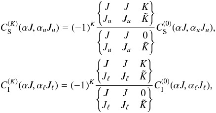 (10)and
in the case of elastic collision:
(10)and
in the case of elastic collision:  (11)The expressions in
braces are the 6j symbol. It is well known that in the case of
electrons with much higher energy than the threshold energy (i.e., under the so-called
Born approximation), the interaction Hamiltonian depends on the dynamical variables of the
atomic system only through the dipole operator (a tensor of rank
(11)The expressions in
braces are the 6j symbol. It is well known that in the case of
electrons with much higher energy than the threshold energy (i.e., under the so-called
Born approximation), the interaction Hamiltonian depends on the dynamical variables of the
atomic system only through the dipole operator (a tensor of rank
 ).
).
As pointed out by Bommier (2009), the inelastic
collision is mainly originated from the atom colliding with the electrons, and the
collision with neutral Hydrogen dominates the elastic collision. Here the elastic
collision means the changes of Zeeman substates under collision. Now we estimate the
inelastic collision rates according to van Regemorter
(1962)’s formula:  (12)where
A(αuJu
→ αJ) is the Einstein coefficient for spontaneous
emission, λcm is the wavelength in unit of cm,
Ne is the density of electron,
Te is the temperature of electron, and
(12)where
A(αuJu
→ αJ) is the Einstein coefficient for spontaneous
emission, λcm is the wavelength in unit of cm,
Ne is the density of electron,
Te is the temperature of electron, and
 is a function of
  .
.
Assume that the colliding particles obey Maxwellian velocity distribution and the
detailed-balance stands, and the following Einstein-Milne relation is valid, ![\begin{equation} \label{eq:13} C_{\rm S}^{(0)}(\alpha J,\alpha_u J_u)=\frac{2J+1}{2J_u+1}C_{\rm I}^{(0)}(\alpha_u J_u, \alpha J)\exp\left[\frac{E(\alpha_u J_u)-E(\alpha J)}{K_{\rm B} T}\right]\cdot \end{equation}](/articles/aa/full_html/2015/01/aa24029-14/aa24029-14-eq83.png) (13)The elastic collision
rates
(13)The elastic collision
rates  can be
obtained in Van der Waals potential approximation (Lamb
& Ter Haar 1971; Landi Degl’Innocenti
& Landolfi 2004),
can be
obtained in Van der Waals potential approximation (Lamb
& Ter Haar 1971; Landi Degl’Innocenti
& Landolfi 2004), ![\begin{equation} \label{eq:14} C_{\rm E}^{(0)}(\alpha J)=1.4\times10^{-10}\left[\left\langle r^2(\alpha J) \right\rangle \right]^{0.4}\left[T\left(1+\frac{1}{\mu}\right)\right]^{0.3}n_{\rm H}. \end{equation}](/articles/aa/full_html/2015/01/aa24029-14/aa24029-14-eq85.png) (14)In the above
expression, T
is the temperature of the atoms, nH the number density of hydrogen atom
in unit of cm-3,
μ the
statistical weight of the atom,
(14)In the above
expression, T
is the temperature of the atoms, nH the number density of hydrogen atom
in unit of cm-3,
μ the
statistical weight of the atom,  the
mean squared radius of the electronic cloud in the level (αJ). The values for
the
mean squared radius of the electronic cloud in the level (αJ). The values for
 can be
deduced through an approximate expression for neutral atoms,
can be
deduced through an approximate expression for neutral atoms,  (15)In the above
equation, Iion is the ionization potential of the
atom, and EαJ the excitation
energy of the (αJ) level. The ionization energy of Mg I ground
state is 7.6462 eV from Kaufman & Martin
(1991) and complied at the NIST atomic spectra database (Kramida et al. 2013).
(15)In the above
equation, Iion is the ionization potential of the
atom, and EαJ the excitation
energy of the (αJ) level. The ionization energy of Mg I ground
state is 7.6462 eV from Kaufman & Martin
(1991) and complied at the NIST atomic spectra database (Kramida et al. 2013).
2.4. Emission coefficients and line profile
The emission and absorption coefficients are the basis of our calculations, and can be
found from Landi Degl’Innocenti & Landolfi
(2004),  (16)where
![\begin{eqnarray} \label{eq:17} \eta_i^{\rm A}(\nu,\vec{\Omega})&=&\frac{h\nu}{4\pi}\mathcal{N}\sum\limits_{\alpha_\ell J_\ell}\sum\limits_{\alpha_u J_u}(2J_\ell +1)B(\alpha_\ell J_\ell\rightarrow\alpha_uJ_u)\nonumber \\ &&\times\sum\limits_{KQK_\ell Q_\ell}\sqrt{3(2K+1)(2K_\ell +1)}\nonumber \\ &&\times \sum\limits_{M_\ell M_\ell 'M_uqq'}(-1)^{1+J_\ell-M_\ell+q'} \nonumber \\ &&\times~\begin{pmatrix}J_u &J_\ell & 1\\-M_u &M_\ell &-q \end{pmatrix}\begin{pmatrix}J_u &J_\ell &1\\-M_u &M_\ell' &-q' \end{pmatrix} \nonumber \\ &&\times~\begin{pmatrix}1 &1 &K\\ q &-q' &-Q \end{pmatrix}\begin{pmatrix}J_\ell &J_\ell &K_\ell \\M_\ell &-M_\ell' & -Q_\ell \end{pmatrix} \nonumber \\ &&\times~{\rm Re}\left[\mathcal{T}_Q^K(i,\vec{\Omega})\rho_{Q_\ell}^{K_\ell}(\alpha_\ell J_\ell)\Phi(\nu_{\alpha_uJ_uM_u,\alpha_\ell J_\ell M_\ell -\nu})\right], \end{eqnarray}](/articles/aa/full_html/2015/01/aa24029-14/aa24029-14-eq97.png) (17)and
(17)and
![\begin{eqnarray} \label{eq:18} \eta_i^{\rm S}(\nu,\vec{\Omega})&=&\frac{h\nu}{4\pi}\mathcal{N}\sum\limits_{\alpha_\ell J_\ell}\sum\limits_{\alpha_u J_u}(2J_u +1)B(\alpha_uJ_u\rightarrow\alpha_\ell J_\ell) \nonumber \\ &&\times~\sum\limits_{KQK_u Q_u}\sqrt{3(2K+1)(2K_u +1)}\nonumber \\ &&\times~ \sum\limits_{M_u M_u'M_\ell qq'}(-1)^{1+J_u-M_u+q'} \nonumber \\ &&\times~\begin{pmatrix}J_u &J_\ell & 1\\-M_u &M_\ell &-q \end{pmatrix}\begin{pmatrix}J_u &J_\ell &1\\-M_u' &M_\ell &-q' \end{pmatrix} \nonumber \\ &&\times~\begin{pmatrix}1 &1 &K\\ q &-q' &-Q \end{pmatrix}\begin{pmatrix}J_u &J_u &K_u \\M_u' &-M_u & -Q_u \end{pmatrix} \nonumber \\ &&\times~ {\rm Re}\left[\mathcal{T}_Q^K\left(i,\vec{\Omega}\right)\rho_{Q_u}^{K_u}\left(\alpha_u J_u\right)\Phi\left(\nu_{\alpha_uJ_uM_u,\alpha_\ell J_\ell M_\ell -\nu}\right)\right]. \end{eqnarray}](/articles/aa/full_html/2015/01/aa24029-14/aa24029-14-eq98.png) (18)In
the above equations, i =
I, Q, U, V, represents the four Stokes parameters
respectively,
(18)In
the above equations, i =
I, Q, U, V, represents the four Stokes parameters
respectively,  is the number density of atoms, B(αℓJℓ
→
αuJu)
and B(αuJu
→
αℓJℓ)
are the Einstein coefficients for absorption and stimulated emission, respectively, and
Φ(ναuJuMu,αℓJℓMℓ
− ν) indicates the complex profile, which is
resulted from the convolution of a Gaussian profile and a Lorentzian profile, given by
is the number density of atoms, B(αℓJℓ
→
αuJu)
and B(αuJu
→
αℓJℓ)
are the Einstein coefficients for absorption and stimulated emission, respectively, and
Φ(ναuJuMu,αℓJℓMℓ
− ν) indicates the complex profile, which is
resulted from the convolution of a Gaussian profile and a Lorentzian profile, given by
 (19)In
the above expression,
(19)In
the above expression,  (20)whereas
H(υ,a) is called Voigt function, and
L(υ,a) is called associated
dispersion profile. The frequency υ is the reduced frequency, and a indicates the damping
constant. The damping constant is given by
(20)whereas
H(υ,a) is called Voigt function, and
L(υ,a) is called associated
dispersion profile. The frequency υ is the reduced frequency, and a indicates the damping
constant. The damping constant is given by  (21)where Γ and Γc are the natural width and the
collision width, respectively, γu and γℓ represent the inverse
lifetimes of the upper and lower levels, respectively, and f is the frequency of
elastic collisions. The Doppler width ΔνD can be estimated through
(21)where Γ and Γc are the natural width and the
collision width, respectively, γu and γℓ represent the inverse
lifetimes of the upper and lower levels, respectively, and f is the frequency of
elastic collisions. The Doppler width ΔνD can be estimated through
 , where
kB is the Boltzmann constant,
M is the
mass of unit atomic weight, and vturb is the microturbulent velocity. In
the following, we use ΔλD = 40 mÅ, resulted
from a temperature of 5755 K
and a micro-turbulent velocity of 1 km s-1.
, where
kB is the Boltzmann constant,
M is the
mass of unit atomic weight, and vturb is the microturbulent velocity. In
the following, we use ΔλD = 40 mÅ, resulted
from a temperature of 5755 K
and a micro-turbulent velocity of 1 km s-1.
In the situation of a weakly polarized atmosphere (ϵI ≫
ϵQ, ϵU, ϵV;ηI
≫ ηQ, ηU, ηV), where
 and
and
 (i =
I, Q, U, V) are the line emission and absorption
coefficients for Stokes parameters, respectively. The emergent fractional polarization is
given by (Trujillo Bueno 2003)
(i =
I, Q, U, V) are the line emission and absorption
coefficients for Stokes parameters, respectively. The emergent fractional polarization is
given by (Trujillo Bueno 2003)  (22)where
X =
Q, U, V. The first term in the righthand side of the
equation represents the contribution of spontaneous emission and the second term
represents the contribution of absorption and dichroism effect. The continuum around the
triplet has a fractional linear polarization Q/I = 0.06%,
given by Fluri & Stenflo (1999) and Stenflo (2005). It is found that the contribution of
the continuum should be added to reproduce the observation profile. For simplicity, we
assume that the continuum emission coefficients and absorption coefficients are constant
around the triplet, the linear polarization of continuum comes from the emission,
(22)where
X =
Q, U, V. The first term in the righthand side of the
equation represents the contribution of spontaneous emission and the second term
represents the contribution of absorption and dichroism effect. The continuum around the
triplet has a fractional linear polarization Q/I = 0.06%,
given by Fluri & Stenflo (1999) and Stenflo (2005). It is found that the contribution of
the continuum should be added to reproduce the observation profile. For simplicity, we
assume that the continuum emission coefficients and absorption coefficients are constant
around the triplet, the linear polarization of continuum comes from the emission,
 (23)In the above
equation,
(23)In the above
equation,  ,
,
 , and
, and
 are the coefficients for
continuum.
are the coefficients for
continuum.
The relationship between the continuum emission coefficient
 and continuum absorption
coefficient
and continuum absorption
coefficient  can be
estimated through the equation under local thermodynamic equilibrium (LTE),
can be
estimated through the equation under local thermodynamic equilibrium (LTE),  (24)where
B(T) is the Planck function at the
frequency resulted from the transition under consideration.
(24)where
B(T) is the Planck function at the
frequency resulted from the transition under consideration.
3. Nonmagnetic field case
The polarization can originate from many mechanisms. In this paper, we emphasize the scattering induced polarization, because in the atmosphere like the chromosphere, scattering plays a very important role in line formation, and can be anisotropic to produce polarization. Besides the anisotropic scattering, many other processes can also produce or change the polarization degree. To see the individual contribution of continuum and collision to the linear polarization clearly, we firstly investigate their roles in the absence of magnetic field, and then discuss the influence of the magnetic field in the next section.
3.1. The role of continuum
The anisotropic incident radiation can induce the atomic polarization. In the scattering
geometry close to the solar limb, the polarization produced by the atomic alignment can be
observed. It is found that if we input anisotropy factors ω1 = 0.1506,
ω2 =
0.1504, and ω3 = 0.1501 for the b4,
b2, and b1 lines,
respectively, which were obtained with the limb darkening coefficients of the continuum
given by Allen (1973), the fractional linear
polarization amplitudes at the line core of the triplet are − 4.43%, 5.98%, and 4.90%. This result shows
a great difference compared with the observation by Stenflo et al. (2000). Obviously, the anisotropy factors derived from the limb
darkening will deviate from that obtained through solving radiative transfer equations in
the line formation region. Thus these values are not suitable to simulate the fractional
linear polarization of strong lines. To fit the observation, we adopt the three anisotropy
factors ω1 =
0.0615, ω2 = 0.016, and ω3 = 0.009 for
the triplet, respectively, and then obtain the fractional linear polarizations
Q/I = 0.165%,
0.172%, and 0.192% for the triplet, respectively, in
absence of collision or magnetic field. These values are very close to the results
presented by Stenflo et al. (2000). As pointed out
by Trujillo Bueno (1999), to get a similar
fractional linear polarization for the triplet, the dichroism contribution needs to be
considered. In our calculation, the atomic alignment coefficients
( ) of lower
levels of the b2 and b1 lines are
found to be 0.481% and −
0.281%, and that of the upper level is 0.156%. It is shown in the lower
levels of the b2 and b1 lines that
the atomic alignment is larger than that of the upper level. This result is close to the
atomic polarization presented by Trujillo Bueno
(2001). The lower levels of Mg I b lines are metastable and actually connect with
the ground level by forbidden transitions. These forbidden transitions will influence the
atomic alignments. As has been seen, the anisotropic illumination in the atmosphere can
lead to large population imbalances in the lower levels of atoms, which are also sensitive
to the weak magnetic field.
) of lower
levels of the b2 and b1 lines are
found to be 0.481% and −
0.281%, and that of the upper level is 0.156%. It is shown in the lower
levels of the b2 and b1 lines that
the atomic alignment is larger than that of the upper level. This result is close to the
atomic polarization presented by Trujillo Bueno
(2001). The lower levels of Mg I b lines are metastable and actually connect with
the ground level by forbidden transitions. These forbidden transitions will influence the
atomic alignments. As has been seen, the anisotropic illumination in the atmosphere can
lead to large population imbalances in the lower levels of atoms, which are also sensitive
to the weak magnetic field.
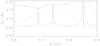 |
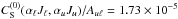
Fig. 1 Influence of continuum on Mg I b triplet Q/I
profile. The absorption coefficient ratio of the continuum to the line
|
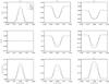 |
Fig. 2 Inelastic collision influence on Q/I
profiles of the Mg I triplet. The solid, dotted, dashed, dot-dashed, and
triple-dot-dashed lines result from the factor ε′ = 1,
100, 500, 1000, and 2000, respectively. In the top panels
ϵQ/ϵI
profiles are plotted, ηQ/ηI
profiles are depicted in the middle panels, and in the
bottom panels ϵQ/ϵI
−
ηQ/ηI
profiles are presented. The continuum intensity corresponds to
|

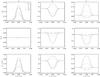 |
Fig. 3 Elastic collision influence on Q/I
profiles of the Mg I triplet. The solid, dotted, dashed, dot-dashed,
triple-dot-dashed, and long dashed lines correspond to the factor ε′ = 0,
0.1, 1, 5, 15, and 30. In the top panels ϵQ/ϵI
profiles are plotted, ηQ/ηI
profiles are depicted in the middle panels, and ϵQ/ϵI
−
ηQ/ηI
profiles in the bottom panels. The continuum intensity corresponds
to |
The fractional polarization profiles can be obtained when we take the contribution of the
continuum into account according to Eq. (11), and we adopt the degrees of continuum polarization according to the theory
of Fluri & Stenflo (1999). We manipulate
the continuum absorption coefficient as a free parameter and the ratios
 ,
and 10-1, where
,
and 10-1, where
 is the absorption coefficient
at line core of the b2 line. The profiles are shown in Fig.
1. It is obvious that the continuum reduces the
polarization at line wings greatly, even though the ratio is low (e.g.,
is the absorption coefficient
at line core of the b2 line. The profiles are shown in Fig.
1. It is obvious that the continuum reduces the
polarization at line wings greatly, even though the ratio is low (e.g.,
 ).
As the continuum absorption coefficient becomes larger and larger, the polarization
amplitudes in the line wings decrease quickly, while those at the line cores keep
unchanged. When the ratio
).
As the continuum absorption coefficient becomes larger and larger, the polarization
amplitudes in the line wings decrease quickly, while those at the line cores keep
unchanged. When the ratio  , the
amplitudes of line core decline markedly. Evidently, the ratio
, the
amplitudes of line core decline markedly. Evidently, the ratio
 gives a
serious contribution to the widths of the fractional polarization profiles. As is well
known, the absorption coefficients depend on the number density of atoms, and the ratio
can be determined through radiative transfer simulations in a realistic model of the quiet
solar photosphere. We found with a trial experience that when
gives a
serious contribution to the widths of the fractional polarization profiles. As is well
known, the absorption coefficients depend on the number density of atoms, and the ratio
can be determined through radiative transfer simulations in a realistic model of the quiet
solar photosphere. We found with a trial experience that when
 , the
widths of observed profiles can be reproduced in the following.
, the
widths of observed profiles can be reproduced in the following.
3.2. The influence of collision
To investigate the influence of collision, we multiply the collision rates for the
triplet by a factor ε′. The factor is set to be 1, 100, 500,
1000, and 2000 for the inelastic collision, and this set results in the ratios of
 ,
1.73 × 10⁻³,
8.65 × 10⁻³,
1.73 × 10⁻², and
2.46 × 10⁻²,
respectively. For the elastic collision, the factor is set to be 0, 0.1, 1, 5, 15, and 30.
Figures 2 and 3
show the variation of ϵQ/ϵI,
ηQ/ηI,
and Q/I profiles with
inelastic and elastic collision rates, respectively. In the case of inelastic collision,
as shown in Fig. 2, when ε′ enhances,
both the ϵQ/ϵI
and ηQ/ηI
profiles decrease, and so do the Q/I profiles. The
inelastic collision obviously reduces the atomic alignments of both the upper and lower
levels only when the super-elastic collision rates are large enough (ε′ ≳
102). This condition is satisfied by a higher electron
density, thus a higher temperature. In contrast to the inelastic collision, we can see
from Fig. 3 that the elastic collision can affect the
Q/I profile even
if the elastic collision rates are small. In detail, when ε′<
10, the lower levels of the b2 and b1 lines are
still polarized. Theoretically, the elastic collision will depolarize both the upper level
and the lower levels of these lines, but in fact the atomic alignment of the upper level
is increased, as evidenced in Fig. 3. That is because
the atomic alignments of the involved levels are coupled as reflected in the statistic
equilibrium equations, while the alignments of the lower levels have a feedback on the
upper level and make the alignment of the upper level increase. Thus the Q/I amplitude of
the b4 line increases with the collision
rates, while the Q/I amplitudes of
the b2 and b1 lines
decrease. When ε′> 10, the
atomic alignments of the lower levels are almost destroyed, which can be seen from
ηQ/ηI
profiles. Then the dichroism effect will not influence the line profiles and the
unpolarized lower level approximation is valid. Thus the atomic polarization of the upper
level declines as the elastic collision rates increase. When the factor is equal to unit,
the polarizations of the lower levels remain and should be taken into account. This is the
basis for the lower level Hanle effect and simulation of the second solar spectrum of Mg I
triplet.
,
1.73 × 10⁻³,
8.65 × 10⁻³,
1.73 × 10⁻², and
2.46 × 10⁻²,
respectively. For the elastic collision, the factor is set to be 0, 0.1, 1, 5, 15, and 30.
Figures 2 and 3
show the variation of ϵQ/ϵI,
ηQ/ηI,
and Q/I profiles with
inelastic and elastic collision rates, respectively. In the case of inelastic collision,
as shown in Fig. 2, when ε′ enhances,
both the ϵQ/ϵI
and ηQ/ηI
profiles decrease, and so do the Q/I profiles. The
inelastic collision obviously reduces the atomic alignments of both the upper and lower
levels only when the super-elastic collision rates are large enough (ε′ ≳
102). This condition is satisfied by a higher electron
density, thus a higher temperature. In contrast to the inelastic collision, we can see
from Fig. 3 that the elastic collision can affect the
Q/I profile even
if the elastic collision rates are small. In detail, when ε′<
10, the lower levels of the b2 and b1 lines are
still polarized. Theoretically, the elastic collision will depolarize both the upper level
and the lower levels of these lines, but in fact the atomic alignment of the upper level
is increased, as evidenced in Fig. 3. That is because
the atomic alignments of the involved levels are coupled as reflected in the statistic
equilibrium equations, while the alignments of the lower levels have a feedback on the
upper level and make the alignment of the upper level increase. Thus the Q/I amplitude of
the b4 line increases with the collision
rates, while the Q/I amplitudes of
the b2 and b1 lines
decrease. When ε′> 10, the
atomic alignments of the lower levels are almost destroyed, which can be seen from
ηQ/ηI
profiles. Then the dichroism effect will not influence the line profiles and the
unpolarized lower level approximation is valid. Thus the atomic polarization of the upper
level declines as the elastic collision rates increase. When the factor is equal to unit,
the polarizations of the lower levels remain and should be taken into account. This is the
basis for the lower level Hanle effect and simulation of the second solar spectrum of Mg I
triplet.
Figure 4 shows the observed and fitted profiles of
the triplet. The dashed lines present the observed profiles by Stenflo et al. (2000), while the solid lines are obtained from the
scattering theory using the collision rates (ε′ = 1) in absence of magnetic field.
One can see that these amplitudes and widths are matched in the line cores when we input
 , and the anisotropy
factors ω1 =
0.131, ω2 = 0.0575, and ω3 = 0.0156.
Because the collisions and the continuum play a depolarization role in the triplet, the
anisotropy factors are set to be larger than the above values to reproduce the profiles.
This simulation leads to the results that of the upper
level is equal to 0.216%, and
those of the lower levels of the b2 and b1 lines are
0.569% and − 0.291%, respectively. It is noticeable
that these results differ a little from the calculation by Trujillo Bueno (2001), and the difference originates from the fact that we input
a large continuum absorption coefficient, which is not considered by Trujillo Bueno (2001).
, and the anisotropy
factors ω1 =
0.131, ω2 = 0.0575, and ω3 = 0.0156.
Because the collisions and the continuum play a depolarization role in the triplet, the
anisotropy factors are set to be larger than the above values to reproduce the profiles.
This simulation leads to the results that of the upper
level is equal to 0.216%, and
those of the lower levels of the b2 and b1 lines are
0.569% and − 0.291%, respectively. It is noticeable
that these results differ a little from the calculation by Trujillo Bueno (2001), and the difference originates from the fact that we input
a large continuum absorption coefficient, which is not considered by Trujillo Bueno (2001).
4. The Hanle effect in the Mg I triplet
In this section, we focus on the role of the magnetic field. It is well known that the magnetic field can modify the polarization via the Hanle effect, which can be used for diagnostics of a weak magnetic field. Especially, the lower level Hanle effect is used for a very weak magnetic field (Landolfi & Landi Degl’Innocenti 1986). Since the lower levels of Mg I b triplet are polarized and the collision cannot destroy the polarization, it satisfies another requirement as a tool to diagnose very a weak magnetic field. In the following, we investigate the Hanle effect on the triplet to see how the weak magnetic field modifies the emergent linear polarization of the Mg I b triplet. Because of the outstandingly different influences on the line cores and wings, we study them separately.
4.1. The Hanle effect at line core
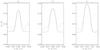 |
Fig. 4 Fractional linear polarization Q/I
profiles of Mg I b triplet close to solar limb (μ = 0.1) in absence
of magnetic field. The dashed lines were measured by Stenflo et al. (2000). The solid lines show the theoretical profiles
obtained with the anisotropy factor ω1 = 0.131, ω2 =
0.0575, and ω3 = 0.0156 for the triplet,
respectively. The continuum intensity corresponds to
|

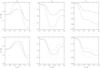 |
Fig. 5 Variation of the emergent Q/I amplitudes with magnetic field vector at the line cores of the Mg I triplet calculated at μ = 0.1. The lines in the top panels are obtained with the magnetic azimuth χB = 90°, and those in the bottom panels with the azimuth χB = 0°. The solid, dotted, and dashed lines result from the magnetic inclination of 30°, 60°, and 90°, respectively. The other parameters are the same as those producing Fig. 4. |
 |
Fig. 6 Hanle effect on the line-core polarization of the Mg I triplet. The lines are obtained close to solar limb (μ = 0.1) in presence of a horizontal magnetic field of various strengths, 0 G (solid lines), 0.005 G (dotted lines), 0.1 G (dashed lines), 1 G (dot-dashed lines), 10 G (triple-dot-dashed lines), and 100 G (long dashed lines). The top six panels show the Q/I and U/I profiles with the azimuth χB = 30°, and the bottom six panels show the Q/I and U/I profiles with the azimuth χB = 0°. The other parameters are the same with those producing Fig. 4. |
Figure 5 shows the variations of Q/I amplitudes at the line cores of the triplet with the magnetic field strengths as well as the inclination θB close to the solar limb (μ = 0.1). The anisotropy factors and collision rates are the same as those producing Fig. 4. The solid, dotted, and dashed lines correspond to θB = 30°, 60°, and 90°, respectively. The top panels are obtained with the magnetic azimuth χB = 0°, and the bottom panels are resulted from χB = 60°.
From Fig. 5, it is easily seen that the
Q/I amplitudes at
the line cores of the triplet are very sensitive to the sub-Gauss range magnetic field
between 0.001 and 0.1 Gauss due to the lower level Hanle effect, and to the Gauss range
between 1 and 10 Gauss due to the upper level Hanle effect. One can see immediately that
the three lines behave differently in the region dominated by the lower level Hanle
effect. The polarization amplitude of the b4 line increases with magnetic field
strength, while those of the b2 and b1 lines
experience reduction. Especially, the b2 line can even get a negative
amplitude. Since the lower level of the b4 line has a zero total angular
momentum (J =
0), the Hanle effect loses its influence on this level, and this line
should not be influenced by a magnetic field between 0.001 and 0.1 Gauss. However, like
the influence of elastic collision discussed above, the alignments of the lower levels of
the b2 and b1 lines can
feed back to the upper level, and thus make the Q/I amplitude of
the b4 increase. When the magnetic field
strength locates between 1 and 10 Gauss, the upper level Hanle effect dominates, while the
lower level Hanle effect becomes saturated. The magnetic sensitivity of these lines are
proportional to the dimensionless coefficient  introduced by Landi Degl’Innocenti (1984), and
 , − 0.5 and 0.1 for the triplet, respectively.
The atomic alignment of the upper level declines with the increasing magnetic field
strength. The b4 line is the most sensitive in this
region and then followed by the b2 and b1 lines. It is
found that the fractional linear polarization of the b2 will increase
with the magnetic field strength, as
, − 0.5 and 0.1 for the triplet, respectively.
The atomic alignment of the upper level declines with the increasing magnetic field
strength. The b4 line is the most sensitive in this
region and then followed by the b2 and b1 lines. It is
found that the fractional linear polarization of the b2 will increase
with the magnetic field strength, as  is negative. When the
magnetic field become stronger than about 10 Gauss, the upper level Hanle effect becomes
saturated.
is negative. When the
magnetic field become stronger than about 10 Gauss, the upper level Hanle effect becomes
saturated.
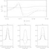 |
Fig. 7 Fractional polarization profiles obtained in the presence of a horizontal magnetic field with χB = 60°. The upper panel shows the whole pattern without continuum, and the bottom panels indicate the line-core profiles with continuum. The pattern varies with the magnetic field of 0 G (solid lines), 0.005 G (dotted lines), 0.01 G (dashed lines), 0.1 G (dot-dashed lines), and 1 G (triple-dot-dashed lines). The anisotropy factors are the same as those resulting in Fig. 1. |
In general, another main result from the Hanle effect is that the polarization plane rotates about the magnetic vector field, and then the observable Stokes U signal appears. When a magnetic field with well-defined inclination and azimuth exists, the Stokes U can be observed due to the rotation. Figure 6 shows both the fractional linear polarization Q/I and U/I profiles of the Mg I b triplet. The profiles in the top six panels are obtained with the magnetic field inclination θB = 90° and azimuth χB = 30°, and those in the bottom six are resulted from θB = 90° and χ = 0°. They show quantitatively how Q/I and U/I profiles vary with magnetic field.
4.2. The Hanle effect in the line wings
Now, we analyze the Hanle effect in the line wings in the presence of a magnetic field. Figure 7 shows the variations of the overall pattern (top panel) and line core profiles (bottom panels) with the magnetic field in the absence of a collision. As proven by Landi Degl’Innocenti & Landolfi (2004), under the assumptions of unpolarized and infinitely sharp lower level in the absence of a collision, the Hanle effect vanishes in the line wings. From the top panel in Fig. 7, however, it is easily seen that magnetic field can influence the whole Q/I profile not only in the line cores with the polarized lower level. The main contribution to the line wings comes from the dichroism effect. This can be explained as follow.
When the dichroism contribution is not considered, the line profile depends on
ϵi, and we have (Landi Degl’Innocenti & Landolfi 2004):
 (25)where
 is the
generalized profile. In the far wings, we have
is the
generalized profile. In the far wings, we have  and
and
 , where Hu =
2πνLgu/
(γu +
γℓ) and
, where Hu =
2πνLgu/
(γu +
γℓ) and
 . Because the
lifetime of the lower level is much longer than that of the upper level, we have
. Because the
lifetime of the lower level is much longer than that of the upper level, we have
 , and the
Larmor frequency dependent of the magnetic field will cancel out in the expression of
ϵi. Therefore, the
magnetic field does not affect the line wings. However, when the dichroism contribution is
considered,
, and the
Larmor frequency dependent of the magnetic field will cancel out in the expression of
ϵi. Therefore, the
magnetic field does not affect the line wings. However, when the dichroism contribution is
considered,  will
contribute to the line profile. In this case, we have a similar relation,
will
contribute to the line profile. In this case, we have a similar relation,  (26)In the far wings, we also
have
(26)In the far wings, we also
have  and
and
 , where Hℓ =
2πνLgℓ/
(γu +
γℓ) and
, where Hℓ =
2πνLgℓ/
(γu +
γℓ) and
 . However,
Hℓ is now one hundred
times bigger than
. However,
Hℓ is now one hundred
times bigger than  in the case
of Mg I b triplet. The magnetic term remains in the dichroism contribution, so the line
wings will be influenced by magnetic field via the dichroism effect. When considering the
contribution of the continuum, the influence on the line wings would not be seen as shown
in the bottom panels of 7.
in the case
of Mg I b triplet. The magnetic term remains in the dichroism contribution, so the line
wings will be influenced by magnetic field via the dichroism effect. When considering the
contribution of the continuum, the influence on the line wings would not be seen as shown
in the bottom panels of 7.
4.3. Hanle-effect diagrams
Hanle-effect diagram can intuitively show the variations of Q/I and U/I amplitudes at line cores with the strength, inclination, and azimuth of the magnetic field. It is a useful tool to determine the magnetic field vector. Figure 8 presents the Hanle-effect diagrams corresponding to the geometry close to the solar limb (μ = 0.1). Each panel corresponds to a fixed magnetic field inclination. The thick lines in all panels correspond to a definite strength, and the azimuth ranges from χB = 0° to χB = 360°. The magnetic field strength is sampled as 0.008, 0.02, 4, and 8 Gauss. The thick solid lines are produced by the azimuth from 0° to 180°, and the thick dotted lines are resulted from 180° to 360°. The thin lines result from the magnetic field strength ranging from 0 to 300 Gauss with a fixed χB. These lines show the increase and decrease of Q/I and U/I amplitudes close to the solar limb, as well as the rotation of polarization plane induced by the Hanle effect. In contrast to the case of the unpolarized lower levels, it is easily seen from Fig. 8 that there will be two interlaced loops corresponding to the lower and upper level Hanle effect. The two loops can be overlapped in the Hanle-effect diagram. Because the loops of the b2 and b1 lines due to the lower level Hanle effect are more conspicuous, especially the b2 line, these two lines are suitable for diagnostic of a sub-Gauss range magnetic field. Another interesting thing is that in a two-level atom model, the lower level Hanle effect does not occur in the transition from Ju = 1 to Jℓ = 0, while in a multi-level magnesium atom model the lower level Hanle effect of the b4 line takes place because of the coupling among atomic alignment with those of the other levels. This line has the most conspicuous upper level Hanle effect loops, thus it is suitable for diagnosing the Gauss range magnetic field.
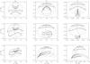 |
Fig. 8 Hanle diagrams show the Q/I and U/I amplitudes in the presence of magnetic field at the line cores of the triplet calculated with μ = 0.1. The top, middle, and bottom panels correspond to θB = 90°, θB = 60°, and θB = 30°, respectively. The thick lines correspond to constant strength magnetic field of 0.008, 0.02, 4, and 8 Gauss with the azimuth 0°<χB< 180° (thick solid line) and 180°<χB< 360° (thick dotted line). The thin lines correspond to the azimuths χB = 0° and χB = 180° thin (dot-dashed line), χB = 30° and χB = 150° (thin dashed line), χB = 60° and χB = 120° (thin dotted line) and χB = 90° (thin solid line). The anisotropy factors, collision rates and continuum are the same as those producing Fig. 4. |
5. Conclusions
We investigate the dependence of scattering induced fractional linear polarization of the magnesium triplet on the continuum, collision, dichroism, and weak magnetic field with the scattering geometry close to the solar limb. It is found that the simplified scattering model in our calculation can fit the main features, such as the amplitudes and widths of the observed Q/I profiles by inputting proper anisotropy factors and continuum, but the inputting values of these parameters are not unique to reproduce these features. This is noticeable when the diagnostic is applied.
The anisotropic illumination in the atmosphere can lead to large population imbalances in levels of the atoms, which are sensitive to the weak magnetic field. In our calculation, the collision rates are not large enough to destroy the population imbalances of the lower levels of the b2 and b1 lines, this is the prerequisite for the lower level Hanle effect and dichroism effect. To get close Q/I amplitudes of triplet to fit the observation, the dichroism effect has to be considered.
In the absence of magnetic field, only Q/I signals are nonzero, and the amplitudes mainly depend on the anisotropy factors. The continuum also can greatly degrade the fractional linear polarization outside the line core, thus significantly influence the widths of the Q/I profiles. On the other hand, the inelastic collision can depolarize in both the line cores and wings. As the inelastic collision rates increase, the atomic polarization of the each level becomes smaller and smaller, and finally disappears. Like the Hanle effect, the elastic collision can influence the atomic alignments. Their difference indicates that the collision cannot lead to any rotation of polarization plane. Theoretically, the elastic collision should decrease the atomic alignments of the upper and lower levels. However, in a multi-level atom model, the atomic alignments can increase in the case of the Mg I triplet. This is because the alignments are coupled in the statistical equilibrium equations. If the elastic collision rates are greater than 5 × 10⁶ s-1, the atomic alignments of lower levels of these lines will be completely destroyed and then the unpolarized lower level approximation is valid.
In the investigation of magnetic field, it is found that the lower level Hanle effect can
influence polarization in the line wings when the dichroism effect is taken into account.
When the continuum becomes strong, the polarization in the line wings cannot be detected
because the continuum greatly reduce the polarization amplitudes of line wings. In the line
cores, the fractional linear polarizations of the triplet are sensitive to the magnetic
field between 0.001 and 0.1 Gauss due to the lower level Hanle effect, and between 1 and 10
Gauss due to the upper level Hanle effect. The most interesting thing is that in the lower
level Hanle effect region, the Q/I amplitude of
the b4 line increases with magnetic field
strength, and that of the b2 can turn from being positive to
negative at a definite magnetic field vector. This phenomenon means that the weak magnetic
field can not only reduce, but also enhance the atomic polarization because the atomic
alignments of different levels are coupled in the statistical equilibrium equations. The
b2
and b1 lines, especially the b2 line, are more
suitable for the diagnostics of a sub-Gauss range magnetic field than the b4 line. In the
upper level Hanle effect dominated region, the b4 line is the most sensitive and then
followed by the b2 and b1 lines, since
their , − 0.5, and 0.1, respectively. Therefore, the
Mg I b triplet can be used for probing the Gauss range magnetic field due to the upper level
Hanle effect, and sub-Gauss range magnetic field due to the lower level Hanle effect.
Acknowledgments
The authors are grateful to Prof. Stenflo for supplying the data and to E. Landi Degl’Innocenti for a careful reading of the manuscript and helpful suggestions. We also thank Dr. Fei Teng for providing the code to compute the complex profile. This work is sponsored by Natural Science Foundation of China(NSFC) under grant numbers 11078005 and 11373065, and the 973 project under grant number G2011CB811400.
References
- Allen, C. W. 1973, Astrophysical quantities, 3rd edn. (University of London, London: The Athlone Press) [Google Scholar]
- Belluzzi, L., & Trujillo Bueno, J. 2011, ApJ, 743, 3 [NASA ADS] [CrossRef] [Google Scholar]
- Belluzzi, L., Trujillo Bueno, J., & Landi Degl’Innocenti, E. 2007, ApJ, 666, 588 [NASA ADS] [CrossRef] [Google Scholar]
- Belluzzi, L., Landi Degl’Innocenti, E., & Trujillo Bueno, J. 2009, ApJ, 705, 218 [NASA ADS] [CrossRef] [Google Scholar]
- Bommier, V. 1980, A&A, 87, 109 [NASA ADS] [Google Scholar]
- Bommier, V. 1997a, A&A, 328, 706 [NASA ADS] [Google Scholar]
- Bommier, V. 1997b, A&A, 328, 726 [NASA ADS] [Google Scholar]
- Bommier, V. 2009, in Solar Polarization 5, in Honor of Jan Stenflo, eds. S. V. Berdyugina, K. N. Nagendra, & R. Ramelli, ASP Conf. Ser., 405, 335 [Google Scholar]
- Fano, U. 1957, Rev. Mod. Phys., 29, 74 [Google Scholar]
- Fluri, D. M., & Stenflo, J. O. 1999, A&A, 341, 902 [NASA ADS] [Google Scholar]
- Fontenla, J. M., Avrett, E. H., & Loeser, R. 1993, ApJ, 406, 319 [NASA ADS] [CrossRef] [Google Scholar]
- Gandorfer, A. 2000, The Second Solar Spectrum: A high spectral resolution polarimetric survey of scattering polarization at the solar limb in graphical representation, Vol. I: 4625 Å to 6995 Å [Google Scholar]
- Gandorfer, A. 2002, The Second Solar Spectrum: A high spectral resolution polarimetric survey of scattering polarization at the solar limb in graphical representation, Vol. II: 3910 Å to 4630 Å [Google Scholar]
- Gandorfer, A. 2005, The Second Solar Spectrum: A high spectral resolution polarimetric survey of scattering polarization at the solar limb in graphical representation, Vol. III: 3160 Å to 3915 Å [Google Scholar]
- Kaufman, V., & Martin, W. C. 1991, J. Phys. Chem. Ref. Data, 20, 83 [NASA ADS] [CrossRef] [Google Scholar]
- Kelleher, D. E., & Podobedova, L. I. 2008, J. Phys. Chem. Ref. Data, 37, 1285 [NASA ADS] [CrossRef] [Google Scholar]
- Kramida, A., Yu. Ralchenko, Reader, J., & and NIST ASD Team. 2013, NIST Atomic Spectra Database (ver. 5.1), available: http://physics.nist.gov/asd, 2014, February 21, National Institute of Standards and Technology, Gaithersburg, MD [Google Scholar]
- Lamb, F. K., & Ter Haar, D. 1971, Phys. Rep., 2, 253 [NASA ADS] [CrossRef] [Google Scholar]
- Landi Degl’Innocenti, E. 1983, Sol. Phys., 85, 3 [NASA ADS] [CrossRef] [Google Scholar]
- Landi Degl’Innocenti, E. 1984, Sol. Phys., 91, 1 [NASA ADS] [CrossRef] [Google Scholar]
- Landi Degl’Innocenti, E. 1996, Sol. Phys., 164, 21 [NASA ADS] [CrossRef] [Google Scholar]
- Landi Degl’Innocenti, E., & Landolfi, M. 2004, Polarization in Spectral Lines (Springer), Astrophys. Space Sci. Lib., 307 [Google Scholar]
- Landolfi, M., & Landi Degl’Innocenti, E. 1986, A&A, 167, 200 [NASA ADS] [Google Scholar]
- Lites, B. W., Skumanich, A., Rees, D. E., & Murphy, G. A. 1988, ApJ, 330, 493 [NASA ADS] [CrossRef] [Google Scholar]
- Manso Sainz, R., & Landi Degl’Innocenti, E. 2002, A&A, 394, 1093 [NASA ADS] [CrossRef] [EDP Sciences] [Google Scholar]
- Manso Sainz, R., & Trujillo Bueno, J. 2010, ApJ, 722, 1416 [NASA ADS] [CrossRef] [Google Scholar]
- Omont, A. 1977, Prog. Quant. Electr., 5, 69 [Google Scholar]
- Stenflo, J. O. 1996, Nature, 382, 588 [NASA ADS] [CrossRef] [Google Scholar]
- Stenflo, J. O. 2003, in Solar Polarization, eds. J. Trujillo-Bueno, & J. Sanchez Almeida, ASP Conf. Ser., 307, 385 [Google Scholar]
- Stenflo, J. O. 2005, A&A, 429, 713 [NASA ADS] [CrossRef] [EDP Sciences] [Google Scholar]
- Stenflo, J. O. 2013, A&ARv, 21, 66 [NASA ADS] [CrossRef] [EDP Sciences] [Google Scholar]
- Stenflo, J. O., & Keller, C. U. 1997, A&A, 321, 927 [NASA ADS] [Google Scholar]
- Stenflo, J. O., Keller, C. U., & Gandorfer, A. 2000, A&A, 355, 789 [NASA ADS] [Google Scholar]
- Trujillo Bueno, J. 1999, in Polarization, eds. K. N. Nagendra, & J. O. Stenflo, Astrophys. Space Sci. Lib., 243, 73 [Google Scholar]
- Trujillo Bueno, J. 2001, in Advanced Solar Polarimetry – Theory, Observation, and Instrumentation, ed. M. Sigwarth, ASP Conf. Ser., 236, 161 [Google Scholar]
- Trujillo Bueno, J. 2003, in Solar Polarization, eds. J. Trujillo-Bueno, & J. Sanchez Almeida, ASP Conf. Ser., 307, 407 [Google Scholar]
- Trujillo Bueno, J. 2009, in Solar Polarization 5: In Honor of Jan Stenflo, eds. S. V. Berdyugina, K. N. Nagendra, & R. Ramelli, ASP Conf. Ser., 405, 65 [Google Scholar]
- Trujillo Bueno, J., Shchukina, N., & Asensio Ramos, A. 2004, Nature, 430, 326 [Google Scholar]
- van Regemorter, H. 1962, ApJ, 136, 906 [NASA ADS] [CrossRef] [Google Scholar]
All Tables
All Figures
|
Fig. 1 Influence of continuum on Mg I b triplet Q/I
profile. The absorption coefficient ratio of the continuum to the line
|
| In the text | |
|
Fig. 2 Inelastic collision influence on Q/I
profiles of the Mg I triplet. The solid, dotted, dashed, dot-dashed, and
triple-dot-dashed lines result from the factor ε′ = 1,
100, 500, 1000, and 2000, respectively. In the top panels
ϵQ/ϵI
profiles are plotted, ηQ/ηI
profiles are depicted in the middle panels, and in the
bottom panels ϵQ/ϵI
−
ηQ/ηI
profiles are presented. The continuum intensity corresponds to
|
| In the text | |
|
Fig. 3 Elastic collision influence on Q/I
profiles of the Mg I triplet. The solid, dotted, dashed, dot-dashed,
triple-dot-dashed, and long dashed lines correspond to the factor ε′ = 0,
0.1, 1, 5, 15, and 30. In the top panels ϵQ/ϵI
profiles are plotted, ηQ/ηI
profiles are depicted in the middle panels, and ϵQ/ϵI
−
ηQ/ηI
profiles in the bottom panels. The continuum intensity corresponds
to |
| In the text | |
|
Fig. 4 Fractional linear polarization Q/I
profiles of Mg I b triplet close to solar limb (μ = 0.1) in absence
of magnetic field. The dashed lines were measured by Stenflo et al. (2000). The solid lines show the theoretical profiles
obtained with the anisotropy factor ω1 = 0.131, ω2 =
0.0575, and ω3 = 0.0156 for the triplet,
respectively. The continuum intensity corresponds to
|
| In the text | |
|
Fig. 5 Variation of the emergent Q/I amplitudes with magnetic field vector at the line cores of the Mg I triplet calculated at μ = 0.1. The lines in the top panels are obtained with the magnetic azimuth χB = 90°, and those in the bottom panels with the azimuth χB = 0°. The solid, dotted, and dashed lines result from the magnetic inclination of 30°, 60°, and 90°, respectively. The other parameters are the same as those producing Fig. 4. |
| In the text | |
|
Fig. 6 Hanle effect on the line-core polarization of the Mg I triplet. The lines are obtained close to solar limb (μ = 0.1) in presence of a horizontal magnetic field of various strengths, 0 G (solid lines), 0.005 G (dotted lines), 0.1 G (dashed lines), 1 G (dot-dashed lines), 10 G (triple-dot-dashed lines), and 100 G (long dashed lines). The top six panels show the Q/I and U/I profiles with the azimuth χB = 30°, and the bottom six panels show the Q/I and U/I profiles with the azimuth χB = 0°. The other parameters are the same with those producing Fig. 4. |
| In the text | |
|
Fig. 7 Fractional polarization profiles obtained in the presence of a horizontal magnetic field with χB = 60°. The upper panel shows the whole pattern without continuum, and the bottom panels indicate the line-core profiles with continuum. The pattern varies with the magnetic field of 0 G (solid lines), 0.005 G (dotted lines), 0.01 G (dashed lines), 0.1 G (dot-dashed lines), and 1 G (triple-dot-dashed lines). The anisotropy factors are the same as those resulting in Fig. 1. |
| In the text | |
|
Fig. 8 Hanle diagrams show the Q/I and U/I amplitudes in the presence of magnetic field at the line cores of the triplet calculated with μ = 0.1. The top, middle, and bottom panels correspond to θB = 90°, θB = 60°, and θB = 30°, respectively. The thick lines correspond to constant strength magnetic field of 0.008, 0.02, 4, and 8 Gauss with the azimuth 0°<χB< 180° (thick solid line) and 180°<χB< 360° (thick dotted line). The thin lines correspond to the azimuths χB = 0° and χB = 180° thin (dot-dashed line), χB = 30° and χB = 150° (thin dashed line), χB = 60° and χB = 120° (thin dotted line) and χB = 90° (thin solid line). The anisotropy factors, collision rates and continuum are the same as those producing Fig. 4. |
| In the text | |
Current usage metrics show cumulative count of Article Views (full-text article views including HTML views, PDF and ePub downloads, according to the available data) and Abstracts Views on Vision4Press platform.
Data correspond to usage on the plateform after 2015. The current usage metrics is available 48-96 hours after online publication and is updated daily on week days.
Initial download of the metrics may take a while.