| Issue |
A&A
Volume 573, January 2015
|
|
|---|---|---|
| Article Number | A64 | |
| Number of page(s) | 10 | |
| Section | The Sun | |
| DOI | https://doi.org/10.1051/0004-6361/201323080 | |
| Published online | 18 December 2014 | |
Wavelet analysis of CME, X-ray flare, and sunspot series
Astrophysics DivisionNational Institute for Space Research,
12227-01
São José dos Campos –SP,
Brazil
e-mail: This email address is being protected from spambots. You need JavaScript enabled to view it.
; This email address is being protected from spambots. You need JavaScript enabled to view it.
,
This email address is being protected from spambots. You need JavaScript enabled to view it.
Received:
18
November
2013
Accepted:
22
October
2014
Abstract
Context. Coronal mass ejections (CMEs) and solar flares are the most energetic transient phenomena taking place at the Sun. Together they are principally responsible for disturbances in outer geospace. Coronal mass ejections and solar flares are believed to be correlated with the solar cycle, which is mainly characterized by sunspot numbers.
Aims. Here, we search for pattern identification in CMEs, X-ray solar flares, and sunspot number time series using a new data mining process and a quantitative procedure to correlate these series.
Methods. This new process consists of the combination of a decomposition method with the wavelet transform technique applied to the series ranging from 2000 until 2012. A simple moving average is used for the time-series decomposition as a high-pass filter. A continuous wavelet transform is applied to the series in sequence, which permits us to uncover signals previously masked by the original time series. We made use of the wavelet coherence to find some correlation between the data.
Results. The results have shown the existence of periodic and intermittent signals in the CMEs, flares, and sunspot time series. For the CME and flare series, few and relatively short time intervals without any signal were observed. Signals with an intermittent character take place during some epochs of the maximum and descending phases of the solar cycle 23 and rising phase of solar cycle 24. A comparison among X-ray flares, sunspots, and CME time series shows a stronger relation between flare and CMEs, although during some short intervals (four–eight months) and in a relatively narrow band. Yet, in contrast we have obtained a fainter or even absent relation between the X-ray flares and sunspot number series as well as between the CMEs and sunspot number series.
Key words: Sun: coronal mass ejections (CMEs) / Sun: activity / methods: data analysis
© ESO, 2014
1. Introduction
It is well known that the Sun presents a cyclic activity, with an average period of 11 years, manifested by phenomena observed both on the solar surface and in the atmosphere. According to Parker (1955), the evolution of a solar magnetic field generated by a dynamo mechanism modulates this cyclic behavior. For instance, sunspot numbers vary according to the cycle phase. One believes the frequency at which transient phenomena, such as solar flares and coronal mass ejections (CMEs), happen are also well correlated to the cycle. The CMEs are mainly associated with changes in the large scale magnetic field and solar flares result from changes in the stronger but smaller scale fields associated with the active regions (Gosling 1993). Although CMEs have been observed in association with solar flares, there is no one-to-one correspondence between them (Harrison 1995).
CME-driven interplanetary disturbances are the prime cause of large nonrecurrent geomagnetic storms, and this had led the CMEs to become a topic of great interest. Almost twenty thousand CMEs have been recorded by the Large Angle and Spectrometric Coronograph (LASCO) experiment on board the Solar and Heliospheric Observatory (SOHO) satellite since 1996. Therefore, a large CMEs series is available for a detailed investigation. In addition, these series of X-ray flares and sunspot numbers are available, for the same period from the Space Weather Prediction Center (SWPC) data archive.
Through the analysis of the CME series, some authors pointed out the existence of patterns in the occurrence of the transient phenomena (Lou et al. 2003; Hady 2004; Lara et al. 2008; Shanmugaraju et al. 2010; Ramesh 2010; Choudhary et al. 2014). In particular, Lou et al. (2003) using a shorter time series (between 1999 and 2003) found signals with periods of 343, 187, 102, 38.3, 36.1 days for the CMEs series, and periods of 259 and 157 days for flare series. Also, using a longer, although discontinuous, CME series from 1996 to 2006, Lara et al. (2008) found a periodicity of 256 days from 1999–2002, between 128–256 days for 2002–2004, which reappeared at the end of 2006, and 32 days in some specific months of 2000, 2001, 2003, and 2005. However, the data series used in these analyses had two gaps (from June 26 to 09 October, 1998; and from December 21, 1998 to February 02, 1999).
More recently, authors have searched periodicities on solar data series in combination with geomagnetic indexes. Most of these studies aim to investigate possible periodicities in each time series and in parallel some correlation or relationship between them. As an example, Kilcik et al. (2011) used data on solar and geomagnetic indexes during the period 1996–2008, although they made use of monthly averaged values. An interesting result they obtained is that the CME speed profile shows a peak at the decay phase of the 23rd solar cycle. Another long-term (century) study, combining solar data as well as simulated extended aa-index series, has been done by Komitov et al. (2010). They suggest the existence of decade cycles on most of those series whose periods are ~55–60 years, ~80 years, and ~120 years, and also that each one probably corresponds to the cycle of a distinct class of an active region.
Other investigations point to a possible relation between CMEs, sunspot/non sunspot regions, and flares (Gopalswamy et al. 2010). These suggest that the weak correlation found between CME-flare occurrence rates with a sunspot number during the maximum phase of the 23rd cycle is due to the fact that CMEs originate at high latitudes. Also, Shanmugaraju et al. (2010) studied 290 CMEs associated with and without type-II related flares. They observed relationships between time characteristic properties of CMEs and flares with type-II, and also between flare strength and CME speed, which are absent in case of the flares without type-II. However, Aggarwal et al. (2008) found no significant correlation between the maximum intensity of X-ray flares with the speed and acceleration of those associated CMEs.
In addition, the wavelet transform (WT) is an adequate tool to analyze non stationary signals in time series at different frequencies. In the context of solar cycles and stellar activity, several investigations have been carried out (Ochadlick et al. 1993; Lawrence et al. 1995; Oliver et al. 1998; Sello 2000, 2003; Lou et al. 2003; Lara et al. 2008; Choudhary et al. 2014). Recently, the relationship between CMEs, solar flares, and flux emergence using just the wavelet power spectrum analysis has been studied by Choudhary et al. (2014). By the periodicity analysis of these events, the authors conclude that CMEs and flares are different types of magnetic explosions requiring different magnetic configuration. Yet, according to same analysis, the flare occurrences are more frequent during the maximum phase of solar cycle when the surface flux is more abundant, while CMEs occurrences are more favorable at the minimum phase when the large-scale surface flux configuration leads to the formation and disruption of the filaments that cause the CMEs.
In this work, we extend the above studies using a continuous CMEs series for the years 2000–2012 to avoid the two main gaps that are present in the LASCO CME catalog. Patterns in occurrence of the transient phenomena can be useful in development of models to predict them. Also, the coherence between the occurrence of these phenomena can help in understanding their origins. Here, we have made use of an innovative data mining process applied to CMEs, X-ray flare, and sunspot number time series. This process permits us to identify patterns hidden in these time series. It combines a decomposition method with a wavelet transform technique applied to a full solar cycle period. We have also used a quantitative method, the wavelet coherence, to look for the way that these series can be interrelated during cycles. Besides, a comparison in terms of patterns, periodicities, or even irregularities identified in these series is presented and discussed.
Data and analysis are described in Sect. 2. Results are presented in Sect. 3. Discussions and final remarks are in the Sect. 4.
2. Data and analysis
Since 1996, CMEs have been systematically observed by the LASCO experiment on board the SOHO satellite (Brueckner et al. 1995; Domingo et al. 1995). In this analysis we use CME data available in the CDAW catalog1 (Yashiro et al. 2004). Here, the data from 1st January 2000 until 31st December 2012 were selected to avoid two major gaps in the LASCO observations: i) 26 June–9 October 1998 and ii) 21 December 1998–2 February 1999. This allowed us to obtain a continuous time series with the daily rate of CMEs for the period 2000–2012. We also have used the data from the SWPC (National Oceanic and Atmospheric Administration–NOAA) to generate the flares and sunspot time series2. The flare time series has only been constructed with data observed in X-ray. All of the time series consist of the number of daily events, and they were taken from the same period as that of CMEs to make the comparisons between them possible. Hereafter, the three series are referred just as CME, XRF, and SSN series.
In order to investigate the existence of relations among these three series as well as to identify periodicities in the series, we adopted the following methodology. Firstly, we perform the simple moving average (SMA), in sequence the wavelet spectrum. In addition, the wavelet coherence analysis has also been performed. According our previous survey, this is the first time that this kind of analysis has been applied for these data. The SMA works as a pre-processing filter in the time series decomposition, while the wavelet analysis is applied to find the characteristic periods. In order to quantify the correlation among the series we have applied the wavelet coherence method. A description of the series decomposition method and a short review about wavelet analysis and the coherence method are presented below.
2.1. Time series filtering
Given a discrete time series x, with N elements, SMA can be calculated by  (1)where M is the number of points in the average.
Considering that T is a vector containing dates corresponding to x, i.e, for xi exists a unique Ti. In this case, the new vector of the dates corresponding to S is given by  (2)In particular, the last term in the vector of Ts is
  (3)where Ts will be spaced by M.
In order to use the SMA as a filter, we create a numerical function, Sint, from the interpolation of the SMA and Ts. This new function is valid in the range ![Mathematical equation: \hbox{$[T_{0}^{s}, T^{s}_{\rm final}]$}](/articles/aa/full_html/2015/01/aa23080-13/aa23080-13-eq15.png) .
.
The final filtering consists of the subtraction of the original signal by Sint(ti,M). In this case, M represents the threshold above which those signals with periods greater than M will not pass. For instance, if one wants to study intra-annual events just consider M = 365. Therefore, the equation for the SMA filtering is  (4)By combining this method with the wavelet analysis, we will perform a more complete characterization of the CMEs series. An example of the CME time series after being filtered is shown in Fig. 1. As can be observed, the smoothed time series is in an interval of [+ σi, −σi] (σi is the standard deviation for each Si). We found that the longer the interval considered, the greater the value of sigma, however, these values did not affect the detection of signals with lower than average periods.
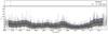 |
Fig. 1 Daily occurrence of CMEs with 365-day moving average superimposed (black line). The shaded area corresponds to the range [+ σ, − σ]. |
2.2. The continuous wavelet transform
Grossmann & Morlet (1984) introduced the wavelet transform (WT) to study non stationary signals. In the context of the solar cycles and stellar activity, WT has been used by some authors (Ochadlick et al. 1993; Lawrence et al. 1995; Oliver et al. 1998; Sello 2000, 2003; Lara et al. 2008; Choudhary et al. 2014). A wavelet (wavelet mother) is a function with zero mean, which is defined in both the frequency, and time spaces (Grinsted et al. 2004).
On the other hand, the idea of continuous wavelet transform (CWT) is to apply the wavelet as a band-pass filter to the time series. The CWT,  , can be applied in a time series, defined by xn, with n = 1,...,N, with uniform time steps Δt, namely (Grinsted et al. 2004)
  (5)with s being the wavelet scale and ψ0 known as the wavelet mother.
In this work, the Morlet wavelet defined as (Grinsted et al. 2004)  (6)is considered where ω0 is the dimensionless frequency and η = st is the dimensionless time. The use of the Morlet wavelet (with ω0 = 6), as a filter, is justified by the fact that it provides a good balance between time and frequency localization (Grinsted et al. 2004).
The square module of the wavelet transform integrated in the time provides the energy contained in all wavelet coefficients of the same scale s (Le & Wang 2003). This function is called global wavelet power spectrum (GWPS) and can be computed as:  (7)To perform the wavelet analysis the tool piwavelet3 (Python Interface for Wavelet analysis) was used and its details can be found in Somoza et al. (2013). The series analysis were carried out with 5% of significance level, as proposed by Torrence & Compo (1998).
A better characterization of the series will be possible with a combination of filtering process and wavelet transform techniques.
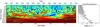 |
Fig. 2 Wavelet power and global wavelet spectra obtained by the CWT applied to the original CME time series. Day of the series, from 01/01/2000 up to 12/31/2012 is at the horizontal axis. The days that appear in the x label are associated with years: day 1000 corresponds to 09/26/2002; day 2000 is 06/22/2005; day 3000 occurred on 03/18/2008 and finally, day 4000 corresponds to 12/13/2010. Vertical axis shows the full band (2–4096 days) of investigations. On the right, the corresponding GWS is shown. |
2.3. Wavelet coherence
The wavelet coherence is used to identify in which frequency band and time range two series are related. In this case, it is necessary to smooth the cross wavelet spectrum before calculating the coherence (Torrence & Compo 1998). Given two time series X and Y, with the respective CWT  and
and  , the wavelet cross power spectrum is given by
  (8)where n is the time index and s the scale. The ∗ represents the complex conjugate.
The square wavelet coherence is defined as the absolute squared value of the wavelet cross power spectrum (WCS), normalized by the smoothed wavelet spectrum (Torrence & Compo 1998)  (9)with S(W) being the timescale smoothing function. The factor s-1 is used to convert the unit of the spectrum in energy density.
The smoothing function is dependent of the scale of the mother wavelet, and is defined by Jevrejeva et al. (2003) as  (10)where Sscale and Stime represent, respectively, the smoothing in the scale and time.
In the case of Morlet’s mother wavelet (Jevrejeva et al. 2003) ![Mathematical equation: \begin{eqnarray} S_{\rm time}(W)|_{s} &=& \left(W(t,s) c_{1}{\rm e}^{-t^{2}/2s^{2}}\right)|_{s} \\[2mm] S_{\rm scale}(W)|_{t} &=& \left(W(t,s) c^{2}\Pi(0.6s)\right)|_{t} \end{eqnarray}](/articles/aa/full_html/2015/01/aa23080-13/aa23080-13-eq48.png) where c1 and c2 are normalization constants and Π is a rectangular function. The factor 0.6 is empirically determined by the length of the Morlet wavelet decorrelation (Torrence & Compo 1998).
where c1 and c2 are normalization constants and Π is a rectangular function. The factor 0.6 is empirically determined by the length of the Morlet wavelet decorrelation (Torrence & Compo 1998).
3. Results
All three data series for the years from 2000 until 2012 are continuous and composed by the daily rate of recorded events. Also, all have been analyzed by the same methodology. This procedure has been adopted to permit the uniformity of data analysis. It also allows for the possibility of comparing the results in terms of time evolution or even studying the correlation among the series.
The data analysis results are presented as power wavelet (WS) as well as global wavelet (GWS) spectra for the series. In these figures, real signals are those inside the black contours observed in the WS with a confidence level of 95%, while the cross-hatched region corresponds to the cone of influence (COI) where the edge effects on time series analysis cannot be ignored. Therefore, the signals inside the COI must be considered virtual signals. The intensities are scaled by distinct colors going from light orange for the weaker components to dark red for the stronger ones. Other colors (e.g., yellow, green, light blue and dark blue) mean no significant real signal is present. Hereafter, real signals are referred to simply as signals. The peaks observed in the GWS correspond to the integrated signal recorded during the full interval of investigation. Then, a more intense band recorded at the WS normally does not correspond to a large peak observed at the GWS. The 95% confidence level is marked on the GWS by the dashed line. The relevance of a given signal can be determined by the equivalent intensity of GWS. When the amplitude of GWS is relatively small, the signals must be considered as residuals.
In the panels intermittent signals are characterized by a relatively short time ( between three to four months) black contoured spots in specific period bands. Contrary to this, other longer scale period bands constitute periodic signals. However, those signals with a time varying period band are referred to as irregular.
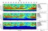 |
Fig. 3 Top panel: wavelet power spectrum obtained by the application of CWT to the SMA smoothed (scale of 365 days) CME time series. Middle panel: the same, using a scale of 180 days. Bottom panel: the same, using a scale of 60 days. On the right, the corresponding GWSs are shown. |
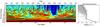 |
Fig. 4 Wavelet power and global wavelet spectra obtained by the CWT applied to the original XRF series. As for previous figures, the corresponding GWS is shown on the right side. |
3.1. CME series
The difficulties regarding the incompleteness of the CME data are overcome here by the selection of a longer continuous series for the years 2000 until 2012. In addition, a new methodology of data reduction was applied to the selected series. As described above, it consisted of the combination of a SMA decomposition with the wavelet technique. For the CME series, the SMA taking M = 365 days is shown in Fig. 1. According to our methodology, the power wavelet spectrum (WS) is the first step for identification of components in these series. Figure 2 can be seen as the WS of CMEs original time series. This figure shows periodic signal bands in the range of 4096 to four days. Considering the peaks observed at the GWS, there is a monotonic decrease in intensity from the ~4000 days signal to shorter periods. As can be seen from both the WS and the GWS, the most intense peaks are in the range of 1024 to 4096. However, these bands are inside the cone of influence (COI), so they are not taking into account. In order from more to less intense and significant GWS peaks, we can see the bands of 512–1024 days, 256–512 days, and 128–256 days, which correspond to the presence of periodic bands as well as intermittent real signals in the WS. Some authors (Lou et al. 2003; Lara et al. 2008; Choudhary et al. 2014) also found these bands. Taking this into account we have used the SMA with intra-annual timescales to further characterize these signals.
The result of the CWT on the CME series after the SMA for 365 day scale is shown in Fig. 3. The signal outside the COI is in the range of 4–512 days. Because of the σ, inside which is the smoothed component, we observe signals beyond 356 days (refer to explanation of Fig. 1). For the GWS, the more intense signals correspond to two intervals in band 128–256 days as observed at the WS. The first, lasting for almost 1000 days, corresponds to the years 2001–2004 while the other, lasting about 600 days, corresponds to the years 2010–2011 at the beginning of 24th solar cycle. In a decreasing order, the second most intense signal is in the band 256–512 days observed during the descending phase of the 23rd cycle. A peak at the band 64–128 days is the last significant one at the GWS. From this band down to shorter scales, the signals acquire an intermittent behavior and can be better observed when SMA is taken at scales shorter than 180 days.
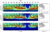 |
Fig. 5 Top panel: wavelet power spectrum obtained by the application of CWT to the SMA smoothed (scale of 365 days) XRF. Middle panel: the same, using a scale of 180 days. Bottom panel: the same, using a scale of 60 days. The corresponding GWSs are shown on the right side. |
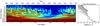 |
Fig. 6 Wavelet power and global wavelet spectra obtained by the CWT applied to the original SSN time series. The GWS is showed on the right side. |
For the 180-day scale, the WS shows that the dominant signal is still on the 256–64 day band (Fig. 3). However, the bottom of Fig. 3 shows that this band of signal is no longer observed at the WS for scales lower than 60 days. Here, only an intermittent signal can be seen. It seems that this intermittent component is present for almost the full 23rd cycle. It can also be observed at the rising phase of the 24th cycle. As shown in Fig. 2, for approximately one year at the end of 23rd cycle no significant component is present at the WS. This gap is longer in the case of smaller scale filtering as can be seen in the middle and bottom panels.
3.2. X-ray flare series
Figure 4 shows the application of CWT to the XRF original time series. Results showed a different behavior in the case of X-ray flares. The spectrum shows the formation of periodic signal bands in the range of 8 to 4096 days. The GWS shows that the most intense signal is at the band from slightly below 2048 up to 4096 days inside the COI. The formation of relatively shorter duration, more concentrated bands in comparison to those observed in the case of Fig. 2 can be seen from the WS. In this case, we can characterize four bands, three of them are relatively faint. The first, lasting for ~two years, is observed during the maximum phase of 23rd cycle in the band 256–512 days. The second, can be seen from the WS for ~3.5 years during the decay phase in the band slightly below 512 days up to 1024 days. The third, observed for ~three years since the beginning of the 24th cycle, is in the band 128–512 days, which extended up to 64 days for half a year. The last and stronger band is also observed at the decay phase of the 23rd cycle and presents an irregular pattern. It started strong approximately in the band 64–128 days lasting ~one year, then became weaker extending up to 256 days and lasting about two years in its middle, and at the end for ~1.5 years is observed drifting to the band about 128–256 days when it strengthened again.
In addition, some short duration (≤few months) spots can also be observed mainly in the decay phase of 23rd as well as in the rising phase of 24th solar cycles where periods of as short as 8 days were registered. We observed a clear gap of about one year in the WS, which seems to separate the two solar cycles.
The GWS exhibits a main intense peak accompanied by a few extremely discrete peaks distributed mainly at scales longer than 32 days.
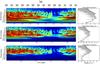 |
Fig. 7 Top panel: wavelet power spectrum obtained by the application of CWT to the SMA smoothed (scale of 365 days) SSN time series. Middle panel: the same, using a scale of 180 days. Bottom panel: the same, using a scale of 60 days. The GWSs are shown on the right side. |
The WS of SMA smoothed XRF series for 365, 180, and 60 days as well as corresponding GWS are exhibited in the three panels of Fig. 5. In this case, it seems that signals are present for the most of the time studied with short duration (≤100 days) gaps and showing wider bands. Another important feature is that the components are broader and more irregular as the filtered scale becomes shorter. For the case of 365 days, the band extends from 8 to about 512 days, while it extends beyond 256 days in the case of 180 days, and beyond 128 days in the case of a 60 day scale. The previously mentioned gap separating the two cycles is also present although ranging from some months at a 365 day scale to about 1.5 year at the 60 day scale. Corresponding GWS exhibit few definite peaks only in the case of those longer scales. Yet, for the WS it seems that some component signals became evident or more prominent after the filtering process.
3.3. Sunspot number series
For the case of SSN, Fig. 6 shows the original time series WS. In this case, a much weaker signal is present than shown in the cases of CME and XRF series. Stronger signals are concentrated inside the COI in the band of 1024–4096 days. Shorter scale signals occurred basically within the band 16–512 days from maximum up to the beginning of the descending phase of the 23rd cycle. One isolated 128–256 days lasting for ~1.5 years is observed at the rising phase of the 24th cycle. This is one of the most intense bands observed in this case. The other is a short duration (~100 days) band observed at the beginning of the descending phase of the 23rd cycle from 16 to a little more than 32 days. A gap longer than four years without any signal is clearly seen in the WS. This gap extends from the descending phase of the last cycle to the beginning of actual cycle rising phase.
Figure 6, at right, corresponding to the GWS showed only one defined peak in the band 16–32 days. Other stronger peaks are observed inside the COI region.
Figure 7 exhibits the SMA smoothed (365, 180, and 60 days) SSN series. All three panels show a band of component signals absent in the original time series WS. This makes the power of the SMA as a filter evident. In addition, it is clear that GWS shows wider, more defined peaks. This is caused basically by the wider (16–512 days) and almost continuous bands of intense signals observed at the WS mainly from the maximum phase up to the middle of descending phase of cycle 23. It can also be observed in a narrower (64–256 days) band at the rising phase of the current cycle. At the smallest scale filtering (60 days), the band became relatively narrower (16–128 days). The gaps between the two cycles are also longer in comparison to those observed in the CME and XRF wavelet power spectra.
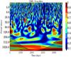 |
Fig. 8 Coherence wavelet applied to CME and XRF data. |
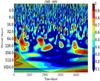 |
Fig. 9 Coherence wavelet applied to CME and SSN data. |
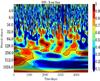 |
Fig. 10 Coherence wavelet applied to SSN and XRF data. |
3.4. Wavelet coherence
One way to quantify relations among the series is through a wavelet coherence process. The main advantage is that it permits the identification of the band and corresponding time interval when this relation is strong. Figures 8–10 show the results of the method applied to pairs of selected series. Basically, the coherence is characterized by relatively narrow and short (less than one year duration) spots in the figures. Figure 8 displays the results obtained by the application to the CME and XRF series. Those red and brown spots in the figure indicate the band and time interval where a stronger relationship between the series was obtained while the blue and dark blue spots indicate the absence of a relationship. Three main spots were observed. The first spot, in the band 16–32 days, lasts about four months at ~2003, while the next spot lasting about twice as long in the band about 64–128 days is observed approximately four months after the end of first. The last significant spot is observed in 2011 approximately in the same band and with same duration as the previous band. This corresponds to the rising phase of the 24th solar cycle. Other shorter duration and smaller scale spots are indicated in the figure. This result indicates that some possible strong relation between these series has a scale of a few months or less, and also that the relations are concentrated to a few years by the descending phase of previous solar cycle and the rising phase of the actual cycle.
Figures 9, 10 show a weaker relation between CME and SSN as well as XRF and SSN series. For both cases there are just a few spots with a strong relation. In the case of CME and SSN (Fig. 9), they are concentrated around the minimum of the last solar cycle. For the case of SSN and XRF, some significant spots concentrated around 128 days and lasting ~1 year was observed (Fig. 10).
3.5. Comparison among the spectra
In general, there are differences among the WS of the three original series as well as SMA filtered series. The WS of CME series presents relatively narrow and middle to long duration continuous bands. Also, a few spot components can be more clearly seen at the smaller scales (60 days) of the SMA filtering. In the case of XRF series WS, there are bands with a more irregular pattern that tend to present relatively short duration and to be spotty toward the smaller scales. These are the stronger signals concentrated along two spots in the descending phase of the 23rd solar cycle. In the SSN series WS, even shorter-duration spotty bands dominate mainly at the maximum and beginning of the descending phase of cycle 23. Besides, a ~1.5 year band in the range 128–256 days shows up at the rising phase of the current solar cycle. One aspect to note regarding the WS of both the original XRF and SSN series is that there is a gap of more than one year between the two solar cycles, which is not defined in the WS of the original CME series. To better analyze this result, the annual number of CMEs during the interval under study were plotted in Fig. 11. We observed that the annual number of CMEs follows the solar cycle trend up to the beginning of the descending phase of the 23rd cycle. Then, we observed two peaks with the second peak being close to the number observed at the maximum of the cycle. The number grows again in the rising phase of the current cycle. The number of CMEs observed stayed at a level of 700 or more per year even at the minimum of the last cycle when the sunspot number remained zero for almost two years.
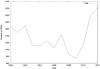 |
Fig. 11 Number of CME events versus year during the period of 2000 to 2012. |
In addition, the smaller the scale of the SMA filtered signal the larger the gap observed between the shorter duration bands. An evident separation can be seen between solar cycles 23 and 24 as identified by the XRF and SSN series. A comparison in terms of wavelet coherence among the selected series indicates that CME and XRF series are better related to each other, although during short time intervals and at the narrow bands of middle to short timescales (8–128 days). This is observed at the beginning of the descending phase of the last cycle and rising phase of the current cycle. We observed a weaker relationship between the CME and SSN series in comparison to the previous case, concentrated in three spots that extend from the end of the 23rd cycle up to rising phase of present solar cycle. The three identified bands extend from 16–32 days, lasting about four months, to 128–256 days, lasting about one year.
A better coherence could be noted between XRF and SSN in the range of 32–256 days. However, the formation of a continuous band was not observed. This fact would indicate a lag between these signals, producing an intermittent intra-annual correlation band.
4. Discussions and final remarks
Using CME, XRF, and SSN continuous series for the interval 2000–2012 we studied the evolution of these phenomena from the maximum phase of the 23rd solar cycle up to the maximum of the present cycle. The study was carried out using wavelet analysis whose advantages are: (1) identification of periodic and non-periodic signals; and (2) determination of when and on which band of periods the signals occur.
However, as could be seen in previous works (Choudhary et al. 2014; Lara et al. 2008), the use of wavelet analysis alone was not sufficient to establish the existence of signals that have lower values than the dominant signal (the solar cycle). In this case it was necessary to develop a new data mining process to stress the signals with a period lower than 365 days. This new methodology consisted of applying a SMA as a high-pass band filter, and therefore, it was possible to identify clearly all bands of signals. Our methodology opens a new window for the development of tools to analyze solar phenomena occurrence within the infra-annual range.
In order to determine if a signal is real or residual it was necessary to investigate the behavior of the GWS, see the small boxes at the sides of Figs. 2–7. We observed that the GWS has shown a strong tendency to weaken as the period decreases. This trend is mainly responsible for masking the less intense signals present in the series and justifies the necessity of using SMA filtering. The signals whose bands were in the region of lower than 95% confidence level (or lower than a threshold) of the GWS were considered as residual. In this way, the GWS is a powerful tool to delimit the real and residual bands.
The application of WS to the selected series permitted us to identify the signal components in those series. For the cases of the CME and XRF series, we observed few, and relatively short, time intervals without any signal. Basically, the signals are observed in the bands within the range 16–1024 days for both WS. In the case of XRF, the signals are more fragmented in time, while in case of CME they are more fragmented in bands. Also, in both cases the shorter the period of the band is, the more fragmented in time the bands are. In the case of the SSN series, signals are restricted to the band 16–256 days and concentrated at spots in the maximum and beginning of the descending phase of the last cycle. One ~2.5 year duration band in the range of 128–256 days is also observed at the rising phase of 24th solar cycle, in good accordance with the results of Choudhary et al. (2014).
Comparing the WS of SSN with the ones of CME and XRF, a gap without any significant signal in the spectrum is clearly observed in the last two, being much larger (several years) in the case of SSN. This seems to reinforce the evidence regarding the anomalous behavior of the 23rd solar cycle particularly at its descending phase (Nandy et al. 2011) suggesting that it is prematurely attained the minimum phase. This means that the last solar cycle suffered some kind of process that stopped the activity a few years earlier than has normally been expected for a regular solar cycle. It could also suggest there is a weaker interdependence between photospheric phenomena and those observed at a higher solar atmosphere, mainly in the corona, than previously supposed. It seems that a randomness dominates the SSN occurrence during the observed gap, which emphasizes the particularity of the last solar cycle. Nevertheless, this is not the case of XRF series, a gap of 1–2 years between the two cycles under study is clearly observed in its WS. However, when the WS is applied to CME series the mentioned gap, if in existence, can hardly be seen. Yet, it is noted that the CMEs occurrence did not stop at the minimum phase of the last solar cycle when the sunspots vanished for more than two years. Here it is worth noting that we are considering just the CME events from the CDAW catalog.
In order to obtain a quantitative comparison among CME, XRF, and SSN, the wavelet coherence was considered. The analysis among the series suggests the following: (1) CME and XRF present a strong relationship although during some short intervals (four–eight months) and in a relatively narrow band. These results must be related to the cases of the most energetic CME events, which are often followed by a flare. This seems to suggest a possible common coronal origin for both phenomena at least during these short time intervals. However, the most of the time we are dealing with independent phenomena. (2) The poor or even faint relation existing between CME and SSN, and between XRF and SSN, respectively, seems to suggest a completely distinct origin for the pair of phenomena under analysis in the sense of solar activity evolution.
A delay between the SSN and flare occurrence has been found by some authors. Through the analysis of monthly sunspot numbers and X-ray flare time series from 1976 to 1999 Wheatland & Litvinenko (2001) observed an approximate six months lag in the flare numbers behind the sunspot numbers. A similar more extended analysis (1976–2008), including less energetic X-ray flares, showed that the time lag varied from nine to five months for the cycles 21 and 23 (Yan et al. 2011). Temmer (2010) attributes this kind of delay to the dynamics of the solar interior, once she noticed an association with a 22 year variation implying a direct link with the magnetic solar cycle. According to Temmer (2010), this can be indicative of a relation with either the solar dynamo or interior processes. Taking this into account, the lack of coherence between flares and SSN series found here can be associated with the delay observed for the solar cycle 23.
A similar delay of six months to one year was also observed for CME and SSN as reported by Robbrecht et al. (2009). These results confirm the lack of coherence between the series observed here, which would be attributed to the fact that CMEs can be originated for quiescent filament regions that can occur at all latitudes. During the solar maximum, however, they occur prominently at high latitudes where sunspots are not found (Gopalswamy et al. 2010).
Our analysis in a certain sense is restricted to relatively middle to small timescales. This is because of the period chosen for the analysis. Strong signals of longer periods inside the COI have been discarded. In this sense, we recommend extending this analysis to longer intervals including some more cycles so as to identify possible periodic signals of longer scales as well as their nature. Finally, to confirm these observed behaviors as characteristic of solar activity and to improve our comprehension more systematic observations of the next solar cycles must be conducted. Particularly, the origin, evolution, and consequences of the solar cycle require further investigation.
To access data see http://cdaw.gsfc.nasa.gov
The piwavelet can be downloaded from the site http://duducosmos.github.io/PIWavelet/. This tool is available under the GNU General Public License Version 3.
Acknowledgments
M.R.G.G. is grateful to CAPES and DAS-INPE for support. E.S.P. would like to thank the Brazilian Agency FAPESP (grant 2012/21877-5) for support. Also, authors thank the CDAW and CUA teams for making CME catalog data available. The CME catalog is generated and maintained at the CDAW Data Center by NASA and Catholic University of America in cooperation with the Naval Research Laboratory. SOHO is a project of international cooperation between ESA and NASA. The authors are grateful to SOHO teams, which are responsible for keeping it in operation for so long. We would also like to thank the referee, who gave us the opportunity to address several issues that were initially overlooked.
References
- Aggarwal, M., Jain, R., Mishra, A. P., et al. 2008, J. Astrophys. Astron., 29, 195 [NASA ADS] [CrossRef] [Google Scholar]
- Brueckner, G. E., Howard, R. A., Koomen, M. J., et al. 1995, Sol. Phys., 162, 357 [NASA ADS] [CrossRef] [Google Scholar]
- Choudhary, D. P., Lawrence, J. K., Norris, M., & Cadavid, A. C. 2014, Sol. Phys., 289, 649 [NASA ADS] [CrossRef] [Google Scholar]
- Domingo, V., Fleck, B., & Poland, A. I. 1995, Sol. Phys., 162, 1 [NASA ADS] [CrossRef] [Google Scholar]
- Gopalswamy, N., Akiyama, S., Yashiro, S., & Mäkelä, P. 2010, Magnetic Coupling between the Interior and Atmosphere of the Sun, eds. S. S. Hasan, & R. J. Rutten, Astrophys. Space Sci. Proc. (Heidelberg, Berlin: Springer), 289 [Google Scholar]
- Gosling, J. T. 1993, J. Geophys. Res., 98, 18937 [NASA ADS] [CrossRef] [Google Scholar]
- Grinsted, A., Moore, J. C., & Jevrejeva, S. 2004, Nonlin. Process. Geophys., 11, 561 [NASA ADS] [CrossRef] [Google Scholar]
- Grossmann, A., & Morlet, J. 1984, SIAM J. Math. Anal., 15, 723 [CrossRef] [MathSciNet] [Google Scholar]
- Hady, A. A. 2004, Meteorol. Geophys. Fluid Dyn., ed. W. Schröder, 97 [Google Scholar]
- Harrison, R. A. 1995, A&A, 304, 585 [NASA ADS] [Google Scholar]
- Jevrejeva, S., Moore, J. C., & Grinsted, A. 2003, J. Geophys. Res., 108, 4677 [CrossRef] [Google Scholar]
- Kilcik, A., Yurchyshyn, V. B., Abramenko, V., et al. 2011, ApJ, 727, 44 [NASA ADS] [CrossRef] [Google Scholar]
- Komitov, B., Sello, S., Duchlev, P., et al. 2010 [arXiv:1011.0347] [Google Scholar]
- Lara, A., Borgazzi, A., Mendes, O. Jr.,, Rosa, R. R., & Domingues, M. O. 2008, Sol. Phys., 248, 155 [NASA ADS] [CrossRef] [Google Scholar]
- Lawrence, J. K., Cadavid, A. C., & Ruzmaikin, A. A. 1995, ApJ, 455, 366 [NASA ADS] [CrossRef] [Google Scholar]
- Le, G., & Wang, J. 2003. Chin. J. Astron. Astrophys., 3, 391 [NASA ADS] [CrossRef] [Google Scholar]
- Lou, Y.-Q., Wang, Y.-M., Fan, Z., Wang, S., & Wang, J. X. 2003, MNRAS, 345, 809 [NASA ADS] [CrossRef] [Google Scholar]
- Nandy, D., Muñoz-Jaramillo, A., & Martens, P. C. H. 2011, Nature, 471, 80 [NASA ADS] [CrossRef] [Google Scholar]
- Ochadlick, A. R., Kritikos, H. N., & Giegengack, R. 1993, Geophys. Res. Lett., 1471 [Google Scholar]
- Oliver, R., Ballester, J. L., & Baudin, F. 1998, Nature, 394, 552 [NASA ADS] [CrossRef] [Google Scholar]
- Parker, E. N. 1955, ApJ, 122, 293 [NASA ADS] [CrossRef] [Google Scholar]
- Ramesh, K. B. 2010, ApJ, 712, L77 [NASA ADS] [CrossRef] [Google Scholar]
- Robbrecht, E., Berghmans, D., & Van der Linden, R. A. M. 2009, ApJ, 691, 1222 [NASA ADS] [CrossRef] [Google Scholar]
- Sello, S. 2000, A&A, 363, 311 [NASA ADS] [Google Scholar]
- Sello, S. 2003, New Astron., 8, 105 [NASA ADS] [CrossRef] [Google Scholar]
- Shanmugaraju, A., Moon, Y.-J., Cho, K.-S., et al. 2010, ApJ, 708, 450 [NASA ADS] [CrossRef] [Google Scholar]
- Somoza, R. D., Pereira, E. S., Novo, E. M. L., & Rennó, C. D. 2013, WIT Transactions on Ecology and The Environment, 178, 1743 [Google Scholar]
- Temmer, M. 2010, SOHO-23: Understanding a Peculiar Solar Minimum, ASP Conf. Ser., 428, 161 [NASA ADS] [Google Scholar]
- Torrence, C., & Compo, G. P. 1998, Bull. Amer. Met. Soc., 79, 61 [NASA ADS] [CrossRef] [Google Scholar]
- Wheatland, M. S., & Litvinenko, Y. E. 2001, ApJ, 557, 332 [NASA ADS] [CrossRef] [Google Scholar]
- Yan, X. L., Deng, L. H., Qu, Z. Q., & Xu, C. L. 2011, Ap&SS, 333, 11 [NASA ADS] [CrossRef] [Google Scholar]
- Yashiro, S., Gopalswamy, N., Michalek, G., et al. 2004, J. Geophys. Res., 109, 7105 [NASA ADS] [CrossRef] [Google Scholar]
All Figures
|
Fig. 1 Daily occurrence of CMEs with 365-day moving average superimposed (black line). The shaded area corresponds to the range [+ σ, − σ]. |
| In the text | |
|
Fig. 2 Wavelet power and global wavelet spectra obtained by the CWT applied to the original CME time series. Day of the series, from 01/01/2000 up to 12/31/2012 is at the horizontal axis. The days that appear in the x label are associated with years: day 1000 corresponds to 09/26/2002; day 2000 is 06/22/2005; day 3000 occurred on 03/18/2008 and finally, day 4000 corresponds to 12/13/2010. Vertical axis shows the full band (2–4096 days) of investigations. On the right, the corresponding GWS is shown. |
| In the text | |
|
Fig. 3 Top panel: wavelet power spectrum obtained by the application of CWT to the SMA smoothed (scale of 365 days) CME time series. Middle panel: the same, using a scale of 180 days. Bottom panel: the same, using a scale of 60 days. On the right, the corresponding GWSs are shown. |
| In the text | |
|
Fig. 4 Wavelet power and global wavelet spectra obtained by the CWT applied to the original XRF series. As for previous figures, the corresponding GWS is shown on the right side. |
| In the text | |
|
Fig. 5 Top panel: wavelet power spectrum obtained by the application of CWT to the SMA smoothed (scale of 365 days) XRF. Middle panel: the same, using a scale of 180 days. Bottom panel: the same, using a scale of 60 days. The corresponding GWSs are shown on the right side. |
| In the text | |
|
Fig. 6 Wavelet power and global wavelet spectra obtained by the CWT applied to the original SSN time series. The GWS is showed on the right side. |
| In the text | |
|
Fig. 7 Top panel: wavelet power spectrum obtained by the application of CWT to the SMA smoothed (scale of 365 days) SSN time series. Middle panel: the same, using a scale of 180 days. Bottom panel: the same, using a scale of 60 days. The GWSs are shown on the right side. |
| In the text | |
|
Fig. 8 Coherence wavelet applied to CME and XRF data. |
| In the text | |
|
Fig. 9 Coherence wavelet applied to CME and SSN data. |
| In the text | |
|
Fig. 10 Coherence wavelet applied to SSN and XRF data. |
| In the text | |
|
Fig. 11 Number of CME events versus year during the period of 2000 to 2012. |
| In the text | |
Current usage metrics show cumulative count of Article Views (full-text article views including HTML views, PDF and ePub downloads, according to the available data) and Abstracts Views on Vision4Press platform.
Data correspond to usage on the plateform after 2015. The current usage metrics is available 48-96 hours after online publication and is updated daily on week days.
Initial download of the metrics may take a while.