| Issue |
A&A
Volume 572, December 2014
|
|
|---|---|---|
| Article Number | A7 | |
| Number of page(s) | 13 | |
| Section | Interstellar and circumstellar matter | |
| DOI | https://doi.org/10.1051/0004-6361/201424395 | |
| Published online | 20 November 2014 | |
The long-period Galactic Cepheid RS Puppis⋆,⋆⋆
III. A geometric distance from HST polarimetric imaging of its light echoes
1
LESIA, Observatoire de Paris, CNRS UMR 8109, UPMC, Université
Paris-Diderot, PSL Research University,
5 place Jules Janssen,
92195
Meudon,
France
e-mail:
This email address is being protected from spambots. You need JavaScript enabled to view it.
2
Department of Astronomy and Astrophysics, 525 Davey Lab.,
Pennsylvania State University, University Park, PA
16802,
USA
3
Space Telescope Science Institute, 3700 San Martin Dr., Baltimore, MD
21218,
USA
4 Konkoly Observatory, 1525 Budapest XII, PO Box 67, Hungary
5
European Southern Observatory, Alonso de Córdova 3107, Casilla 19001,
Santiago 19,
Chile
6
Universidad de Concepción, Departamento de
Astronomía, Casilla
160-C, Concepción,
Chile
7
Astrophysics Research Institute, Liverpool John Moores University,
Liverpool Science Park,
146
Brownlow Hill Liverpool,
L3 5RF,
UK
8
IRAP, UMR 5277, CNRS, Université de Toulouse,
14 av. E. Belin,
31400
Toulouse,
France
9
Observatoire de Genève, Université de Genève,
51 Ch. des
Maillettes, 1290
Sauverny,
Switzerland
Received: 13 June 2014
Accepted: 29 July 2014
Abstract
As one of the most luminous Cepheids in the Milky Way, the 41.5-day RS Puppis is an analog of the long-period Cepheids used to measure extragalactic distances. An accurate distance to this star would therefore help anchor the zero-point of the bright end of the period-luminosity relation. But, at a distance of about 2 kpc, RS Pup is too far away for measuring a direct trigonometric parallax with a precision of a few percentage points with existing instrumentation. RS Pup is unique by being surrounded by a reflection nebula whose brightness varies as pulses of light from the Cepheid propagate outward. We present new polarimetric imaging of the nebula obtained with HST/ACS. The derived map of the degree of linear polarization pL allows us to reconstruct the three-dimensional structure of the dust distribution. To retrieve the scattering angle from the pL value, we consider two different polarization models, one based on a Milky Way dust mixture and one assuming Rayleigh scattering. Considering the derived dust distribution in the nebula, we adjust a model of the phase lag of the photometric variations over selected nebular features to retrieve the distance of RS Pup. We obtain a distance of 1910 ± 80 pc (4.2%), corresponding to a parallax of π = 0.524 ± 0.022 mas. The agreement between the two polarization models that we considered is good, but the final uncertainty is dominated by systematics in the adopted model parameters. The distance we obtain is consistent with existing measurements from the literature, but light echoes provide a distance estimate that is not subject to the same systematic uncertainties as other estimators (e.g., the Baade-Wesselink technique). RS Pup therefore provides an important fiducial for calibrating the systematic uncertainties of the long-period Cepheid distance scale.
Key words: stars: individual: RS Puppis / circumstellar matter / techniques: polarimetric / stars: variables: Cepheids / dust, extinction / scattering
Based on observations made with the NASA/ESA Hubble Space Telescope, obtained at the Space Telescope Science Institute, which is operated by the Association of Universities for Research in Astronomy, Inc., under NASA contract NAS 5-26555. These observations are associated with program #13454.
Table 1 and Appendix A are available in electronic form at http://www.aanda.org
© ESO, 2014
1. Introduction
Thanks to their very high intrinsic luminosity, long-period Cepheids are observable in distant galaxies and can be used as standard candles up to tens of megaparsecs. As a consequence, Cepheids are a central rung in the extragalactic distance scale (Freedman & Madore 2010; Riess et al. 2009, 2011). The long-period Cepheid RS Puppis (HD 68860) is one of the most massive and intrinsically bright stars of its class in the Galaxy. Its physical properties are comparable to the Cepheids observed to measure cosmological distances, which makes it an important fiducial for calibrating the Cepheid distance scale (see, e.g., Riess et al. 2011; Freedman et al. 2001; Sandage et al. 2006).
RS Pup is unique among Galactic Cepheids by being embedded in a reflection nebula, discovered by Westerlund (1961). Havlen (1972) demonstrated that features within the nebula show light variations at the Cepheid’s pulsation period and argued that these “echoes” could be used to derive a geometric distance. Kervella et al. (2008) used the EMMI imager on the 3.6-m ESO NTT telescope to monitor the light variations of the nebula and determine phase lags of the brightest knots in the reflection nebula. They determined a very precise geometric distance to RS Pup of 1992 ± 28 pc. However, Bond & Sparks (2009) point out that this conclusion was based on an assumption that the knots were predominantly located near the plane of the sky. Such an assumption is unlikely to be the case because the high efficiency of forward scattering means that the knots will lie mainly in front of the star.
Bond & Sparks (2009) do, however, point out that polarimetric imaging could be used to determine a purely geometric distance to RS Pup, because the degree of linear polarization of dust-scattered light is maximum for a ~90° scattering angle. This method had originally been proposed by Sparks (1994) as a method for determining distances to extragalactic supernovae and was one of the arguments for including a polarimetric capability in the Advanced Camera for Surveys (ACS) that was installed in the Hubble Space Telescope (HST) in 2002. The method was actually first applied by Sparks et al. (2008) to the spectacular light echo illuminated by the Galactic luminous transient V838 Monocerotis. The polarimetric distance determined for V838 Mon was verified independently by main-sequence fitting for a sparse open cluster associated with the star (Afşar & Bond 2007).
In this paper we present new ACS polarimetric imaging of the RS Pup nebula, from which we obtain a precise geometric distance. Unlike the case of the single outburst of V838 Mon, RS Pup emits a periodic cycle of light maxima every 41.5 days, leading to a set of nested echoes. These echoes are dominated by dust lying in front of the star. By adopting a polarization scattering model, however, we are able to recover the geometric distance.
2. Observations and data processing
2.1. Instrumental setup and raw data reduction
We observed RS Pup using the Wide Field Channel (WFC) of the ACS onboard the HST. We selected the high-throughput F606W filter, which was combined successively with the three polarizers (0, 60, and 120°). ACS/WFC polarimetry with this filter is now well-calibrated (Cracraft & Sparks 2007; Sparks et al. 2008). This wavelength range is an optimal choice in terms of scattered light intensity, because the high flux from the yellow supergiant combines with the efficient scattering from the dust. Since the field-of-view (FoV) of the ACS/WFC polarizers (an unvignetted circular FoV with diameter 70′′) is smaller than the ~3′ size of the RS Pup nebula, we positioned the Cepheid near the edge of the FoV, and we focused on a bright, high polarization area of the nebula that was identified by Kervella et al. (2012). Seven epochs of polarimetric imaging, equally spaced throughout a single pulsation cycle of RS Pup, were obtained between 2010 March 25 and April 29. We also spent one HST orbit to obtain a two-filter (F435W and F606W) unpolarized image of the entire nebula in the full WFC field, in order to map the faint extensions of the nebula and accurately estimate the sky background. Finally we also obtained two observations of nearby bright point spread function (PSF) stars of two different colors matching the color range of the Cepheid. The complete list of the exposures obtained in our ten-orbit HST program is presented in Table 1.
The raw images were processed following the procedure described in Sparks et al. (2008). The data reduction started by retrieving the flt files, which are flat-fielded but not distortion-corrected, from the MAST archive. There were two flat fielded files for each visit/filter/polarizer combination. Each set of two flt files were processed using the astrodrizzle1 software (Gonzaga et al. 2012) that performed distortion corrections, removed cosmic rays, and shifted and aligned all of the images of RS Pup. In some cases, the task tweakreg was used to ensure better alignment of the images. All of the visits were set to align with the POL0 observation of the first HST visit. In order not to affect any of the polarizer parameters, such as polarization angle or degree, the sky background was not subtracted from the images, and there was no rotation applied during this step. The images were drizzled to the native ACS/WFC scale of 0.05 arcsec/pixel. The result of this processing was a single image for each polarizer (POL0V, POL60V, and POL120V) for each of the visits (Table 1).
2.2. PSF wings and sky background subtraction
The subtraction of the stray light from the very bright central star and the sky background is an important step of the processing, because their contributions affect the derived polarimetric quantities. To estimate the stray light from RS Pup, we considered the observations of the two PSF reference stars, HD 71670 (hereafter PSF-Red) and HD 68111 (PSF-Blue), of similar apparent brightness to RS Pup (Table 2).
Properties of the PSF calibrators of RS Pup.
We created a reference PSF image for each polarizing filter POL0V, POL60V, and POL120V. We then masked the background stars and artifacts present in the PSF images using a combination of our two reference stars. The resulting combined PSF image (that is devoid of background stars) is affected by a high noise level, as well as the combination of the artifacts present in the individual images. Directly subtracting these images from RS Pup’s frames results in a degraded signal-to-noise ratio (S/N), particularly in the low flux parts of the images. To mitigate this effect, we computed the radial median profile of this PSF image over concentric rings. Based on this smooth median profile, we generated a synthetic PSF image that presents a clean and better estimated background level. Residual ghost images of the telescope pupil are present in the RS Pup images and not in the PSF composite images. Their position and morphology is complex and variable, but they are easily identified and are not used in the polarization analysis.
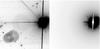 |
Fig. 1 Image of the PSF star HD 68111 (PSF-Blue) in the F606W+POL0V polarizing filter setup (left) and the derived composite synthetic PSF (right). |
The sky background of the images of RS Pup is difficult to estimate, because the light-scattering, variable surface brightness circumstellar nebula covers most of the WFC1 aperture. We however identified two sufficiently extended regions that present the lowest background level. We checked that the average flux level in these areas is consistent with the sky background measured at greater distances from RS Pup, using the wide field image obtained on 2010 March 26 in the F606W filter (WFCENTER aperture setup). We subtracted this constant background uniformly from the polarized images of RS Pup.
The flux normalization factor of the PSF star to the changing brightness of RS Pup was computed using the synthetic light curve of the Cepheid in the F606W filter for each HST observing phase. This light curve of RS Pup was derived from a combined fit of multicolor photometry (see Kervella et al., in prep., hereafter Paper IV) and considered a magnitude m(F606W) = 7.67 ± 0.01 for the PSF-Blue star (HD 68111). The flux-normalized PSF images were subtracted from the RS Pup images for each polarization filter separately. An example of the result of this subtraction is presented in Fig. 2. Residual artifacts are present in the subtracted image. They include, in particular, diffraction and saturation spikes, as well as several pupil ghosts, but their angular extent is limited, and they are located outside of the regions of interest (see Sect. 4.1).
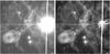 |
Fig. 2 First observing epoch of RS Pup before (left) and after (right) the subtraction of the PSF wings and sky background, with the same gray scale (proportional to the square root of the flux count). The “double doughnut” feature in the lower left quadrant of the image is an optical artifact. |
2.3. Polarimetric quantities
The Stokes parameters I, Q, and U, the degree of linear polarization pL, and the polarization electric-vector position angle in detector coordinates θD were derived from the PSF subtracted images of RS Pup using the approach described by Sparks et al. (2008) and Sparks & Axon (1999). The expression of these quantities are presented in Appendix A. We adopted the position angles of the electric vectors of the polarizers and the photometric throughputs calibrated by Biretta et al. (2004). The pL values were debiased considering the photometric S/N using the bias correction listed in Table A.1 of Sparks & Axon (1999). The uncertainties were propagated to the Stokes parameters starting from the photometric error bars produced by the ACS processing pipeline. The pL and θD values were computed only where the photometric S/N in the unpolarized flux image is sufficiently high (I/σ(I) > 5), to avoid a divergence in the normalization by I. As the nebula is illuminated by the Cepheid (single source), the polarization electric-vector position angle θD is always perpendicular to the dust-star direction over the whole surface of the nebula, as already observed by Kervella et al. (2012).
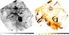 |
Fig. 3 Average maps of the Stokes I (left, in e− s-1) and degree of linear polarization pL (right), computed over the seven observing epochs of RS Pup (north is up and east to the left). |
2.4. Phase map and photometry of the nebula
2.4.1. Period and reference epoch
For matching correctly the phases of the light echoes occurring in the nebulosity around RS Pup, knowledge of the accurate value of the pulsation period of the Cepheid is essential. Therefore, the pulsation period and its variations have been determined with the method of the O−C diagram (Sterken 2005). A discussion of the determination of the period of RS Pup for the epochs of our HST/ACS observations will be presented in Paper IV. We adopt a period P = 41.5117 days for the epoch of our ACS observations (2010).
A simple fit of the light curve to our ACS photometry is the most direct way to obtain a high precision date for the maximum light relevant for our analysis, as we are insensitive to possible random period variations (Berdnikov et al. 2009). This approach also presents the advantage to avoid any shift in the maximum light epoch between the F606W filter and the ephemeris available in the literature (usually in the V or B bands). Unfortunately, the central region close to RS Pup is heavily saturated in the ACS images, and it is particularly difficult to directly obtain accurate photometry for the star. But the ghost image of the telescope pupil that is present south-southwest of the star in Fig. 3 (left panel) provides an unsaturated proxy to the stellar flux. Although the equivalent photometric transmission of this pupil image is unknown, its stability is sufficient for deriving accurate relative fluxes from our seven observing epochs. Through a fit of the synthetic F606W light curve of RS Pup to the measured relative photometry of the pupil ghost image, we obtain a heliocentric Julian date T0 = 2 455 252.64 ± 0.07 for the maximum light (Fig. 4). It should be noted that Anderson (2014) demonstrates that the pulsation of RS Pup shows some degree of cycle-to-cycle variability in radial velocity amplitude and phase, but at a level that does not affect the present light echo analysis.
2.4.2. Phase offsets over the nebula
The propagation of the light echoes in the nebula of RS Pup are clearly visible in the
sequence of our seven epochs of ACS imaging2. We
adopt a two-step approach to determine the phase offset of the nebular features.
Following Kervella et al.
(2008), we first adjust the synthetic light curve of RS Pup in the
F606W filter normalized to unit amplitude and zero average
f(φ) using a three-parameter
model:  (1)where
φi is the phase of
the considered observation i (i.e., the phase of the Cepheid itself at the
corresponding epoch), A is the amplitude of the photometric variation at
coordinates (α,δ) in the nebula, f0 the average
photometric flux, and Δφ the phase offset relative to the Cepheid’s
photometric variation. For each position over the nebula, we therefore derive a triplet
(A,f0,Δφ).
(1)where
φi is the phase of
the considered observation i (i.e., the phase of the Cepheid itself at the
corresponding epoch), A is the amplitude of the photometric variation at
coordinates (α,δ) in the nebula, f0 the average
photometric flux, and Δφ the phase offset relative to the Cepheid’s
photometric variation. For each position over the nebula, we therefore derive a triplet
(A,f0,Δφ).
As discussed by Kervella et al. (2012) and Havlen (1972), the scattering layer must be geometrically thin as we observe contrasted light echoes over most of the nebula. But its non-zero thickness nevertheless causes the shape of the light curve to change over the nebula. A very thin layer produces a high contrast curve that is mostly identical to the light curve of the Cepheid, while a thicker dust layer will result in phase smearing and a smoother, lower amplitude curve with a shifted maximum flux phase. Such a shift in the maximum flux phase Δφ could affect our distance determination. We therefore computed a second photometric fit using smoothed versions of the light curve of RS Pup for those regions of the nebula where the first fit yielded a reduced χ2> 1. These light curves were computed using a boxcar moving average. We increased progressively the boxcar width from 0.1 to 1.0 in phase (with a 0.1 step), stopping for each pixel when the reduced χ2 became lower than 1. This process produced new triplets (A,f0,Δφ) for each point over the nebula, as well as a value of the boxcar width. We note that this second fitting step effectively reduces the χ2 of the three-parameter model fit, but its effect is weak in terms of phase offset over most of the nebula. The resulting maps of the average flux f0, amplitude A and phase offset Δφ are presented in Fig. 5.
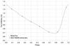 |
Fig. 4 Synthetic light curve of RS Pup (blue curve) in the F606W filter with the ACS photometry derived from the ghost image of the telescope pupil (open circles) phased with T0 = 2 455 252.64 (JD⊙) and P = 41.5117 days. |
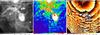 |
Fig. 5 Maps of the average flux f0 (left panel, in e− s-1), amplitude A (central panel, in e− s-1), and phase offset Δφ (right panel) of the photometric variations observed in the southern quadrant of the nebula of RS Pup. The FoV is 68.3′′ × 68.3′′, with north up and east to the left. |
3. Polarization model
The overall geometrical configuration of the scattering layer is shown in Fig. 6. The computation of the position of the dust layer with respect to the star is based on the determination of the scattering angle θ from the degree of linear polarization pL. We consider two models here: (1) a physical model of the Milky Way dust developed by Draine (2003), scaled to the observed pmax value; and (2) a parametrized Rayleigh scattering model with two parameters (pmax,θmax).
3.1. Maximum degree of linear polarization pmax
For both polarization models (Rayleigh and Draine), the maximum degree of polarization pmax can be estimated from our ACS observations. But in practice, determining the maximum value of a statistical distribution is a relatively difficult task. We cannot simply read the maximum value of pL in the pixels of our map (≈ 55%), because the measurements are affected by a statistical uncertainty. We would therefore obtain too high a value, biased by the statistical dispersion. To estimate the true value of pmax, we analyzed the statistical distribution of the values of pL in the nebula. We sorted the measured values of pL by increasing value, and binned them into percentile bins of width 1%. The sample we considered contains 21 600 pixels with an S/N on pL higher than 10, i.e. 216 pixels per percentile bin. A third-degree polynomial fit to the 0−10% bin median values is shown in Fig. 7 as a dashed curve. Its intercept at 100% percentile gives a pmax = 54%. However, the highest percentile bins (0−3%) show a deviation compared to the general linear trend that is present over the 3−10% percentiles. The reason for this deviation is that the average statistical error bar of each pL measurement in our sample is σ = 3.7%. This means that if we consider the 1% highest pL values that exhibit a 53% median visibility, we essentially sample the positive statistical fluctuations of pL values that are in reality (on the sky) around 50%. In other words, the median values in the highest percentiles (0−3% corresponding to pL = 48 to 53%) show the statistical “tail” of the Gaussian distribution of the highest pL values rather than the true distribution of the pL values on the sky.
To avoid a bias on the measured value of pmax, we therefore adopt a quadratic polynomial fit and ignore the three highest pL bins (0 to 3%), which are shown with open symbols in Fig. 7. The intercept of the quadratic polynomial fit to the resulting measurements is pmax = 51.5%, as shown by the solid curve in Fig. 7. To estimate the uncertainty in this fitting procedure, we also adjusted a linear model, which gives an intercept of 50%. Considering the range of results between the linear, quadratic, and third-degree polynomial fits, we adopt pmax = 51.5% ± 2.0% for our two polarization models (Milky Way dust and Rayleigh) that is shown in Fig. 7.
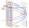 |
Fig. 6 Geometry of the light echoes in the dust surrounding RS Pup. |
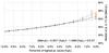 |
Fig. 7 Median pL values observed in the nebula of RS Pup in 1% bins as a function of the percentile of highest values. The attached vertical segments show the full range of values of pL in each bin. The orange segment on the vertical axis shows the adopted uncertainty range for pmax = 51.5% ± 2.0%. |
We can compare this value with the observations by Kervella et al. (2012) using the VLT/FORS instrument. A map of the degree of linear polarization measured in the nebula of RS Pup by these authors in the V band is presented in Fig. 8. The regions of highest polarization labeled (A), (B), and (C) are located at approximately 1.5′ from the Cepheid. The median polarization and standard deviation of the pL values measured over these windows is (A) = 50.0% ± 3.6%, (B) = 50.2% ± 4.7%, and (C) = 49.0% ± 4.7%. These maximum values are in good agreement with the pmax value we measure in the HST/ACS images in the same wavelength range. Another comparison is the maximum value of pL measured by Sparks et al. (2008) in the circumstellar nebula of V838 Mon. These authors observed pmax ≈ 50% (see also Sects. 3.2 and 3.4), again in good agreement with our value. The case of the nebula of V838 Mon is particularly interesting as the dust is distributed relatively homogeneously around the star. This means that the maximum polarization pmax is actually reached in the nebula, as all scattering angles are present in the echo.
The value of pmax that we derive is formally a lower limit, since all scattering angles may not be present in the ACS FoV. However, we put forward the hypothesis here that a fraction of the dust we observe is present down to the plane of the sky and beyond, i.e. that it is not all confined between us and the Cepheid. Considering the overall shape of the nebula and of its distant extensions (Fig. 8), this assumption appears reasonable. We note that we have not observed pL values both in our VLT/FORS and HST/ACS higher than pmax = 51.5% in a statistically significant way. We therefore consider our value of pmax in the following as a measurement and not as a lower limit.
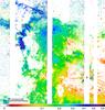 |
Fig. 8 Map of the degree of linear polarization pL in the nebula of RS Pup from VLT/FORS observations (Kervella et al. 2012). |
3.2. Milky Way dust polarization model
The Milky Way (MW) dust model presented in Fig. 53 of Draine (2003) for RV = 3.1 gives pmax = 25.5% for θmax = 90° at 616.5 nm. This wavelength is the closest to the ACS WFC F606W filter, because the range covered by this filter is ≈ 470−710 nm, with λC = 590 nm and Δλ = 230 nm.
The difference between the pmax value of the MW dust model (24−27%) with what we observe (51.5%) points at a difference in the dust grain properties. In the theoretical Rayleigh scattering case, for which the typical size of the particles R is small compared to the wavelength λ, we expect that pmax → 100% and θmax → 90°, with pmax decreasing with increasing R/λ. Although the variation may not be strictly monotonic for large grains (Shen et al. 2009), the high observed pmax indicates that the dust grains surrounding RS Pup and V838 Mon are probably smaller in size than the average MW mixture considered by Draine (2003).
We derive a suitable polarization model for our observations by scaling the MW dust models to match the pmax = 51.5% value that we measure on the nebula of RS Pup. We took the bandpass of the F606W filter into account by computing the average of the relevant polarization models from Draine (2003), weighted as a function of wavelength by the photometric throughput of the ACS WFC+F606W as listed in the ACS Handbook (Ubeda et al. 2012). We thus obtained the pL(θ) model shown in Fig. 9. It is interesting to note that the model we derive using our independently determined value of pmax (Fig. 9) provides an excellent match to the observed polarization function of V838 Mon derived by Sparks et al. (2008).
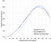 |
Fig. 9 Milky Way dust (pmax = 51.5%, solid black curve) and Rayleigh (pmax = 51.5%, θmax = 92°, dashed curve) models of the linear polarization degree pL(θ). The observed polarization function measured by Sparks et al. (2008) for the dust surrounding V838 Mon is shown as a blue curve. |
3.3. Rayleigh polarization model
The dependence of the linear polarization degree pL on the scattering angle θ may be assumed to be given by the classical Rayleigh polarization phase function (White 1979). For theoretical Rayleigh scattering, pmax = 100% is reached in the plane of the sky, i.e. the imaginary plane perpendicular to the line of sight containing RS Pup, for which θmax = 90° (Fig. 6). However, the maximum values of pL observed in astrophysical context are lower than 100%, and the angle of maximum polarization may be different from 90°. We introduce two parameters to account for possible deviations in the actual dust scattering properties from the Rayleigh polarization law, the maximum degree of linear polarization pmax and the angle of the maximum polarization θmax. This is the approach selected by Sparks et al. (2008) for their study of V838 Mon’s light echo. The expression of pL can be written as 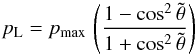 (2)where pmax is the maximum degree of linear polarization, and
  is the scaled scattering angle defined as
 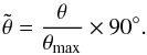 (3)The pL(θ,pmax,θmax) function reaches its maximum value pmax for θ = θmax (Fig. 9). For our Rayleigh polarization model, we adopt the measured value of pmax = 51.5% ± 2.0% (Sect. 3.1).
The second parameter θmax of our polarization model cannot be measured directly from the observations. This parameter, estimated by Sparks et al. (2008) to be in the range 90° ± 5°, is the main source of systematic uncertainty in their distance estimate of V838 Mon. From our broadband MW dust model presented in Sect. 3.2, we derive θmax(MW,F606W) = 92°. Over the full visible range (0.4−0.8 μm), the value of θmax for the models by Draine (2003) varies between 90° and 95°, with a standard deviation of ≈ 2°. We thus adopt an uncertainty range of θmax = 92° ± 2° for our Rayleigh polarization model of RS Pup’s nebula.
3.4. Polarization models from the literature
As mentioned above, the polarization model is the leading systematic uncertainty in this investigation. It is thus useful to compare the model adopted here with others from the literature. For their study of the Homunculus nebula surrounding η Car, Schulte-Ladbeck et al. (1999) assumed a pL(θ) function peaking around θmax ≈ 97° at pmax ≈ 34% in the V band (WFPC2+F555W). This assumed value of θmax is 2.5σ away from our scaled MW dust model, but the actual function depends on the composition of the dust that is probably different in the Homunculus and the average MW interstellar medium. The massive nebula surrounding the red supergiant VY CMa was observed in polarimetric imaging by Jones et al. (2007) using HST/WFPC2 and the F550M and F658N (Hα) filters. The measured pL values reach 75%, with an assumed pL(θ) function peaking around θmax = 100°.
The observations of the circumstellar disk of AU Mic by Graham et al. (2007) using HST/ACS in the F606W filter were reproduced well by a Rayleigh polarization function peaking at θmax = 90°. These authors simultaneously fitted the Henyey & Greenstein (1940, 1941, hereafter H-G) phase function, and the linear polarization function pL(θ) to the data. They obtained pmax = 53 ± 3% for their single-component H-G model with a strong forward scattering, in good agreement with the value we derive for RS Pup. Sahai et al. (1999) observed the protoplanetary nebula Roberts 22 using HST/WFPC2 polarimetry in the F606W filter. They measure comparable maximum pL values (40−50%) to what we find in the nebula of RS Pup, and they reproduce their observations with a distribution of low albedo grains and a Rayleigh scattering phase function (θmax = 90°).
That we observe a very similar value of pmax in RS Pup’s nebula to the one in Sparks et al. (2008) for V838 Mon gives us confidence that the dust surrounding these two stars share physical properties. As shown by Tylenda & Kamiński (2012) and Kervella et al. (2012), these dust clouds were not created by mass loss from the two stars, but are the remnants of interstellar dust clouds. The dust envelopes of η Car and VY CMa have a different origin, since they were recently formed by mass loss from the central stars.
The experiments by Volten et al. (2007) at a wavelength of 633 nm show very high degrees of linear polarization (up to pL ≈ 50% to 100%) on light scattered by fluffy dust grains. Such grains are expected to be good analogs of the interstellar dust. The high pL values are interpreted as the signature of the scattering from the small-size grains in the aggregates, while the phase function shape is determined by the size distribution of the aggregates. The measured maximum polarization angle θmax values in the different samples studied by these authors are consistently very close to 90°. The high pL values observed in V838 Mon and RS Pup’s nebulae therefore point to the presence of such aggregates of very small grains and lend support to our adopted range of 92° ± 2° for θmax. Photochemical processing of the dust grains as they are heated by the central star’s radiation may also lead to the destruction of the larger, porous, and fluffy grains to form a population of very small grains with scattering properties closer to the Rayleigh hypothesis. This process was probably more efficient in the past than it is now, as the main sequence progenitor of RS Pup was a hot B-type star producing strong ultraviolet radiation.
4. Distance determination from the light echoes
4.1. Selection of suitable nebular features
The overall morphology of the RS Pup nebula is relatively complex (Fig. 10), with a number of knots and filaments spread over the apparent extent of the dust. To obtain a higher S/N on the pL map, we averaged the seven observing epochs and binned the resulting map by 2 × 2 pixels. A temporal variability of pL is detectable between our seven observing epochs. This is caused by the propagation of the parabolic light echo surfaces (Fig. 6) into the three-dimensional circumstellar material, which results in different scattering angles as a function of time (hence different values of pL). This variability is observed mostly in the low polarization regions (close to the central star), which do not constrain the altitude of the scattering material above the plane of the sky properly. For this reason, they do not affect our distance fit, and we considered the average map of pL for our distance analysis.
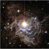 |
Fig. 10 Color composite view of the circumstellar nebula of RS Pup assembled from the ACS WFC images in the F435W and F606W filters obtained on 2010 March 26 (color rendition: NASA, ESA, Z. Levay, and the Hubble Heritage Team STScI/AURA-Hubble/Europe Collaboration). The maximum light echoes are visible as blue rings owing to the hotter temperature of the central star around its maximum light. North is up and east to the left, and the FoV is 2.9 × 2.9 arcmin. |
For the selection of the suitable areas of the RS Pup images for the distance fit, we first determined the FoV limits (the pointing of the telescope slightly changes between epochs) and excluded all the regions that are affected by artifacts (pupil ghosts, diffraction spikes, etc.), as well as the background stars and their associated halos. We also masked the pixels for which the 3-parameter fit (Sect. 2.4.2) did not converge properly. This resulted in a fraction of selected pixels corresponding to 48% of the full ACS frame. After smoothing the pL map using a 7 × 7 pixel box, we selected the regions that have a sufficiently high polarimetric S/N  . This resulted in the selection of 25% of the original pixels. We then selected the highest polarized flux pixels, i.e. the pixels for which
  (Fig. 11). This selection ensures both that the selected regions are high enough above the noise background (high I) and that the scattering occurs essentially in a single dust layer located relatively close to the plane of the sky (high pL). This selection process resulted in the identification of 4000 suitable pixels (≈ 0.4% of the full ACS frame with 2 × 2 binning).
While the presence of contrasted light echoes over most of the nebula indicates that the scattering layer is generally thin, the observed behavior of the echoes varies depending on the location. For instance, the relative amplitude of the photometric variation in the nebula is lower than the Cepheid’s own variation. When this amplitude is much lower than the Cepheid’s, the dust may be distributed in a thick layer or even in several superposed layers. In this case, deriving a single phase lag is difficult and may lead to biases. Therefore, we tried selecting pixels in the nebula that show a high relative photometric variation amplitude. However, this procedure essentially selected only pixels with high values of I × pL. We therefore preferred to keep the selection process simple to avoid biases, and we did not apply this additional selection criterion.
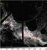 |
Fig. 11 Map of the polarized flux I × pL in the nebula of RS Pup (in e− s-1). The red contours enclose the regions that were selected for the distance fit. The artifacts and background stars have been masked, and the yellow cross marks the position of RS Pup. The dashed yellow circles mark 30′′ and 60′′ angular separations from the Cepheid, and the FoV is 68.3′′ × 68.3′′ with north up and east to the left. |
4.2. Light echo model
When fitting for the distance, we employ the measured pL map to infer the scattering angle θ(pL) from both the Milky Way and Rayleigh polarization models defined in Sect. 3. We assume in the following that the scattering angle is lower than or equal to θmax, i.e. that the scattering occurs in the forward direction. At visible wavelengths, forward scattering is far more efficient than backward scattering, which means that the dust we observe around RS Pup is mainly located between us and the Cepheid, rather than behind the star. We also consider that the physical size of the nebula (≈ 1 pc) is negligible with respect to the distance to RS Pup (≈ 2 kpc). The altitude Z of the scattering dust above the plane of the sky (as shown in Fig. 6) is derived through ![Mathematical equation: \begin{eqnarray} Z_{[\mathrm{pix}]}(p_\mathrm{max}, \theta_\mathrm{max}) = \tan\left[ 90^\circ - \theta(p_{\rm L}, p_\mathrm{max}, \theta_\mathrm{max}) \right]\ r_{[\mathrm{pix}]} \end{eqnarray}](/articles/aa/full_html/2014/12/aa24395-14/aa24395-14-eq117.png) (4)where θ(pL,pmax,θmax) is the selected polarization model, and r[ pix ] the apparent angular separation between the dust feature and the central star. For the MW dust model (Sect. 3.2), we consider that pmax = 51.5% ± 2.0% and θmax is not a free parameter. For the Rayleigh model (Sect. 3.3), we additionally assume θmax = 92° ± 2°. The resulting altitude Z is in the same physical unit as the projected separation r expressed here in pixels for convenience.
(4)where θ(pL,pmax,θmax) is the selected polarization model, and r[ pix ] the apparent angular separation between the dust feature and the central star. For the MW dust model (Sect. 3.2), we consider that pmax = 51.5% ± 2.0% and θmax is not a free parameter. For the Rayleigh model (Sect. 3.3), we additionally assume θmax = 92° ± 2°. The resulting altitude Z is in the same physical unit as the projected separation r expressed here in pixels for convenience.
The linear length C[ m ] of the variation cycle of RS Pup propagating in space with the velocity c is given by C[ m ] = P[ s ]c[ m s-1 ] where P = 41.5117 days is the photometric variation period. The linear size ℓ[ m ] corresponding to one pixel at RS Pup’s distance d is given by ![Mathematical equation: \begin{equation} \ell_{[\mathrm{m}]}(d) = \epsilon_{[\mathrm{''}]}\ d_{[\mathrm{pc}]}\ \mathrm{AU}_{[\mathrm{m}]} \end{equation}](/articles/aa/full_html/2014/12/aa24395-14/aa24395-14-eq128.png) (5)where ϵ = 0.0993 arcsec pix-1 is the plate scale of the 2 × 2 pixel binned ACS images, d[ pc ] is the distance to RS Pup in parsecs, and AU[ m ] represents the length of one astronomical unit expressed in meters. The angular scale C[ pix ] (expressed in pixels) of one variation cycle at RS Pup’s distance d, is then given by the expression:
(5)where ϵ = 0.0993 arcsec pix-1 is the plate scale of the 2 × 2 pixel binned ACS images, d[ pc ] is the distance to RS Pup in parsecs, and AU[ m ] represents the length of one astronomical unit expressed in meters. The angular scale C[ pix ] (expressed in pixels) of one variation cycle at RS Pup’s distance d, is then given by the expression: ![Mathematical equation: \begin{equation} C_{[\mathrm{pix}]}(d) = \frac{C_{[\mathrm{m}]}}{\ell_{[\mathrm{m}]}} = \frac{C_{[\mathrm{m}]}}{\epsilon_{[\mathrm{''}]}\ d_{[\mathrm{pc}]}\ \mathrm{AU}_{[\mathrm{m}]}} \cdot \end{equation}](/articles/aa/full_html/2014/12/aa24395-14/aa24395-14-eq133.png) (6)The linear radius R(x,y) between RS Pup located at position (x⋆,y⋆) and the dust at the apparent position (x,y) in the nebula is then computed from
(6)The linear radius R(x,y) between RS Pup located at position (x⋆,y⋆) and the dust at the apparent position (x,y) in the nebula is then computed from ![Mathematical equation: \begin{equation} R_{[\mathrm{pix}]}(x,y, p_\mathrm{max}, \theta_\mathrm{max}) = \sqrt{ \left( x-x_\star \right)^2 + \left(y-y_\star\right)^2 + Z(x,y)_{[\mathrm{pix}]}^2}. \end{equation}](/articles/aa/full_html/2014/12/aa24395-14/aa24395-14-eq137.png) (7)As discussed by Couderc (1939; see also Sugerman 2003; Bond & Sparks 2009), the model phase lag Δφ(x,y) of the photometric variation of the dust is given by
(7)As discussed by Couderc (1939; see also Sugerman 2003; Bond & Sparks 2009), the model phase lag Δφ(x,y) of the photometric variation of the dust is given by ![Mathematical equation: \begin{equation} \Delta \phi_\mathrm{model}(x,y,p_\mathrm{max}, \theta_\mathrm{max},d) = \frac{R_{[\mathrm{pix}]}(x,y) - Z_{[\mathrm{pix}]}(x,y)}{C_{[\mathrm{pix}]}(d)}\cdot \end{equation}](/articles/aa/full_html/2014/12/aa24395-14/aa24395-14-eq139.png) (8)
(8)
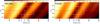 |
Fig. 12 Map of the reduced χ2 of RS Pup’s distance adjustment for the scaled Milky Way dust polarization model (left panel) and the scaled Rayleigh scattering polarization model with θmax = 92° (right panel), as a function of the adopted pmax value (vertical axis). The white rectangle indicates horizontally the distance range found in the literature and vertically the adopted pmax uncertainty range (51.5% ± 2.0%). The white dots show the position of the minimum χ2 for pmax = 49.5, 51.5 and 53.5%. The color scale shown above the map is a function of the square root of the reduced χ2 value. |
4.3. Distance computation
To derive the distance d of RS Pup, we minimize the following expression as a function of d: ![Mathematical equation: \begin{equation} \chi^2(d, p_\mathrm{max}, \theta_\mathrm{max}) = \sum_{(x,y) \in S}{\left[ \frac{\Delta \Phi}{\sigma(\Delta \phi)} \right]^2} \end{equation}](/articles/aa/full_html/2014/12/aa24395-14/aa24395-14-eq144.png) (9)where S is the selected pixel sample as described in Sect. 4.1 and
(9)where S is the selected pixel sample as described in Sect. 4.1 and  (10)In this expression, the phase difference γ is defined as γ = |Δφmodel − Δφ| and { ... } represents the fractional part. This procedure is necessary since the phase values derived from the ACS images are wrapped, i.e. Δφ ∈ [ 0,1 ]. Owing to the complexity of the nebula and the fact that the dust distribution is not continuous, it is not possible to directly unwrap the measured phase lags from our data to retrieve the integral number N of phase lag cycles. This was already the case for the study by Kervella et al. (2012). We thus consider ΔΦ as the distance between the model and the observations. The uncertainties associated to the parameters of the polarization model (pmax,θmax) are systematic, so we derive their contributions separately.
Before the computation of the χ2 minimization, we smoothed the polarization map using a 11 × 11 pixel moving average, and the phase lag map using a 3 × 3 pixel moving average to improve the S/N. Following Ubeda et al. (2012), we adopt a minimum uncertainty on the degree of linear polarization pL of ±1%, and we set a minimum uncertainty on the phase lag of ±0.01. In the highest photometric S/N regions of the nebula, the statistical uncertainties that we derive for these two quantities are very small, and fixing these minimum uncertainties ensures that we do not underestimate them.
As discussed in Sect. 5.1, the published distance estimates for RS Pup range from ≈ 1800 pc (Storm et al. 2011) to ≈ 2100 pc (Fouqué et al. 2003). We therefore considered for the χ2 minimization a range of distances of 1500 to 2400 pc.
4.3.1. Distance from the Milky Way dust polarization model
The scaled MW dust model that we adopt has a single parameter pmax = 51.5% ± 2.0% (Sect. 3.2). Figure 12 (left panel) shows the map of the reduced χ2 of the distance adjustment using this model. We estimated the statistical uncertainty by bootstrapping the distribution of the best-fit distances obtained on each selected pixel for the pmax = 51.5% model. Thanks to the relatively large number of pixels, it is negligible (<10 pc) compared to the systematic uncertainties.
The pmax uncertainty domain and the distance range from the literature are represented as a rectangular box in Fig. 12. The lowest χ2 region is elongated and tilted with respect to the two axes, because of the correlation between pmax and the distance. Over the adopted range of pmax values, the minimum χ2 is reached between 1850 and 1970 pc, i.e. ±60 pc around a best-fit distance of 1910 pc for pmax = 51.5%. Formally, our MW dust model has only one parameter pmax, but there is also an implicit systematic uncertainty on the angle of maximum scattering, computed by Draine (2003) using a specific dust mixture. As discussed in Sect. 3.3, we adopt a range of ±2° around the maximum polarization angle of 92°, which translates into a systematic uncertainty of ±2.5% on the distance (Sect. 4.3.2), or ±50 pc.
We conclude that the best-fit distance for RS Pup considering the scaled MW dust polarization model is d(MW) = 1910 ± 10stat ± 60pmax ± 50θmax pc. Combining all uncertainties, we therefore obtain d(MW) = 1910 ± 80 pc (4.2%).
4.3.2. Distance from the Rayleigh polarization model
The overall structure of the χ2 map for the Rayleigh polarization model (Fig. 12, right panel) shows minor differences with the one obtained for the MW dust model. The tilt of the minimum χ2 regions with respect to the axes is slightly different, and the width of the minimum χ2 “valley” is narrower. These two effects are due to the more peaked polarization curve as a function of the scattering angle (see Fig. 9), which makes the scattering angle less correlated with the value of pmax. The best fit distance for pmax = 51.5% and θmax = 92° is 1940 pc. The range of distances corresponding to pmax varying from 49.5% to 53.5% is 1890 to 1980 pc, i.e. ±50 pc.
According to Sparks et al. (2008), for an instantaneous outburst, the dependence of the distance d with the angle of maximum polarization θmax follows the relation: 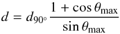 (11)where d90° is the distance obtained for θmax = 90°. From this expression, and considering the adopted range of θmax values (92° ± 2°), we obtain a relative uncertainty of ±3.5% on the distance. The case of RS Pup is, however, slightly different, because we observe several occurrences of the light echoes simultaneously in the nebula, which we fit together using our model. The light curve of RS Pup is also not perfectly sharp. We checked the uncertainty introduced by the θmax parameter by computing χ2 maps for the 1-σ interval (90−94°). From these maps, we obtain a relative uncertainty on the best-fit distance of ±2.5%, corresponding to ±50 pc, which we adopt as the systematic uncertainty associated with the maximum polarization angle (also for the distance estimated using the MW dust model).
The best-fit distance for RS Pup with the Rayleigh dust polarization model is therefore d(Rayleigh) = 1940 ± 70 pc (3.6%).
4.4. Discussion and final distance
We obtain distances of d = 1910 ± 80 pc and 1940 ± 70 pc for our two scattering models, respectively, which are in good agreement with each other. The Milky Way dust polarization model is based on a more realistic physical model, and it is also found to be applicable to the light echoes observed by Sparks et al. (2008) around the red transient V838 Mon. We therefore prefer the MW model over the Rayleigh scattering model.
A cut through the χ2 map for the MW dust model with pmax = 51.5% and the extremes of the adopted uncertainty range (49.5% and 53.5%) is presented in Fig. 13. This curve presents a second minimum for d = 2220 pc. This behavior is caused by the dust features suitable for the distance adjustment being located relatively far from RS Pup (Fig. 11), between 30″ and 1′ from the Cepheid. This implies that the integral number of variation cycles N between their photometric variation and that of the Cepheid is typically six (between 4 and 8). We therefore have an integral uncertainty of one sixth of the distance, i.e. ≈ 300 pc, owing to the phase lag aliasing. While the shorter distance of ≈ 1600 pc can be excluded based on the χ2 criterion, the larger distance ≈ 2200 pc gives a fit of similar quality as 1910 pc. We discuss in Sect. 5.1 why we believe that the larger distance can be excluded, and we propose a final distance value of d = 1910 ± 80 pc (4.2%) for RS Pup.
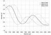 |
Fig. 13 Reduced χ2 curve of the distance fit for the scaled Milky Way dust polarization model with pmax = 49.5%, 51.5%, and 53.5%. |
Observationally determined distances of RS Pup (“IRSB” stands for “infrared surface brightness”).
5. Discussion
5.1. Existing distance estimates
A list of the published measurements of the distance of RS Pup is presented in Table 3. The values derived from the Baade-Wesselink (BW) technique are listed with the assumed value of the projection factor (p-factor). The p-factor is a multiplicative parameter used to convert radial velocities into pulsational velocities to determine distances with the BW technique. It is particularly important because the distances derived from the BW technique scale linearly with the p-factor. This parameter has only been measured for two Cepheids: for δ Cep (P = 5.37 d, p = 1.27 ± 0.06) by Mérand et al. (2005) and for OGLE-LMC-CEP-0227 (P = 3.80 d, p = 1.21 ± 0.05) by Pilecki et al. (2013).
The measured BW distances in Table 3 show both a statistical dispersion and a systematic dispersion caused by different choices for the p-factor value. As shown in Table 3, most authors based their BW distance determination on the linear period-p-factor relation established by Hindsley & Bell (1986, 1989): p = 1.39−0.03log P, which gives p = 1.341 for RS Pup. The distance of 1 568 pc published recently by Groenewegen (2013) departs significantly from the other estimates, but this is due to the choice by this author of a particularly low value of the p-factor (p = 1.112). Scaling this estimate to the “canonical” p = 1.341 results in a distance of 1 891 pc, in good agreement with our light echo measurement and the other values from the literature. Excluding the Hipparcos parallax values (which are unreliable for such a distant star) and the relatively low precision BW measurement by Gieren et al. (1993), the weighted average of the measurements listed in Table 3 results in a distance of 1960 pc, with a standard deviation of 125 pc. For homogeneity, we scaled all the BW distances using a p-factor of 1.341 for this averaging. As proposed by Anderson (2014), the cycle-to-cycle modulation of the radial velocity amplitude of RS Pup probably contributes to the scattering of the BW distances in the literature. It should be noted that the listed measurements are not fully independent of each other, since they often rely on the same sets of observations (photometry, radial velocimetry).
The overall agreement of the existing BW distance estimates with the value we derive in the present work is therefore good within their uncertainties. This indicates that no significant bias is present on the distances determined with the BW technique for long-period Cepheids. We will discuss the implications of the distance we derive for RS Pup on its p-factor in Paper IV.
As discussed in Sect. 4.4, a minimum is present in the χ2 maps of our light echo model fit (Fig. 12) for a distance of ≈ 2200 pc (Fig. 13). Such a large distance for RS Pup appears unlikely since it would result in an unrealistically high value for the p-factor. Scaling the average distance of 1960 pc from the literature (p = 1.341) to a distance of 2200 pc would result in a p-factor of 1.51. Such a value is higher than the purely geometrical component of the p-factor (1.5), i.e. the straight integration of the velocity field over a sphere of uniform brightness (Nardetto et al. 2007). A p-factor higher than 1.5 would imply that the limb of the star is brighter than the center of its apparent disk. While this cannot be formally excluded, it is not foreseen by existing models, in particular for long-period pulsating stars like RS Pup (see, e.g., the references in Nardetto et al. 2014). In addition, a distance of 2200 pc would result in a significant deviation by RS Pup from the period–luminosity relations (Sect. 5.2) by ≈ 0.25 mag. Such a shift would significantly exceed the intrinsic dispersion of the P-L relation, particularly at infrared wavelengths (σ(K)≈0.11 Madore & Freedman 2012), and make RS Pup a uniquely bright Cepheid, which appears unlikely.
5.2. RS Pup and the period–luminosity relation
Considering the intensity-mean magnitudes of ⟨ V ⟩ = 7.119, ⟨ B ⟩ = 8.645, and ⟨ B − V ⟩ = 1.528 determined from our recent SMARTS photometry (Paper IV) and using the values of E(B − V) = 0.457 ± 0.009(Fouqué et al. 2007), RV = 3.1, and the distance of 1910 ± 80 pc, the absolute magnitudes of RS Pup turn out to be ⟨ MV ⟩ = −5.70 ± 0.09 and ⟨ MB ⟩ = −4.63 ± 0.09. Figure 14 shows the position of RS Pup in the V band period-luminosity diagram, together with the sample of Galactic Cepheids for which trigonometric parallaxes were obtained by Benedict et al. (2007) using the HST Fine Guidance Sensor (FGS). The absolute magnitudes in this plot have been taken from these authors. In this diagram the linear PL relation derived by Benedict et al. (2007) from the FGS sample and the one from Fouqué et al. (2007) are shown for comparison. The agreement of RS Pup’s position with both calibrations of the PL relation is satisfactory at the ≈ 1σ level, although the slope of the relation from Benedict et al. (2007) appears slightly too shallow. We reserve a more detailed discussion of this point to a forthcoming article (Paper IV).
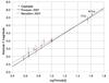 |
Fig. 14 Period–luminosity diagram in the V band showing the position of RS Pup. The relations by Fouqué et al. (2007) and Benedict et al. (2007) are shown as solid and dashed lines, respectively. |
6. Conclusion
The combination of ACS imaging polarimetry and photometry of the circumstellar nebula of RS Pup allowed us to measure the distance of this fiducial long-period Cepheid, which we find to be d = 1910 ± 80 pc (4.2%) corresponding to a parallax π = 0.524 ± 0.022 mas. The major part of the associated uncertainty comes from the adopted polarization model for the light scattered off the nebular dust. Consistent results were obtained for scaled versions of a Rayleigh scattering and a Milky Way dust model. The derived distance is compatible with existing Baade-Wesselink (BW) estimates from the literature, assuming a projection factor p ≈ 1.3 (see Paper IV for a detailed discussion). This agreement between fully independent techniques gives confidence that the current calibration of the Cepheid distance scale is not affected by a large bias, since it is mainly based on the application of various implementations of the BW technique. As discussed by Bennett et al. (2014), reaching a 1% concensus on the value of the Hubble constant H0 from high and low redshift indicators requires an unbiased calibration of the Cepheid distance scale. This can only be obtained from multiple and independent techniques, and in this context, our determination of the distance of RS Pup from its remarkable light echoes offers an original contribution.
Considering the angular scale of the light echoes of RS Pup in the plane of the sky (≈4″ at 1.9 kpc), the measurement technique we applied is in principle applicable up to much greater distances. The angular resolution of the HST should allow distance measurements up to 20 kpc, possibly even up to the Magellanic Clouds, for a configuration similar to RS Pup. Unfortunately, this Cepheid may be the only star of its class in the Milky Way to be so closely embedded in a dusty reflection nebula4. As discussed by Kervella et al. (2012), the bulk of the material surrounding RS Pup is not the result of mass loss from the star itself, but consists of an interstellar dust cloud in which the Cepheid is temporarily embedded. Such an association of a long-period Cepheid and a nebula is therefore the result of the unlikely conjunction of a short-lived massive star (M≈9.2±0.5 M⊙, from Anderson et al. 2014) in a brief phase of its evolution into the classical instability strip, and a dense interstellar dust cloud with a suitable geometry. The shape of the RS Pup nebula determined from polarimetry indicates that the high luminosity of the Cepheid and its progenitor affected the dust distribution, carving a large cavity in the dust cloud. The Cepheid may therefore clear the remaining dust over the next few million years, making the light echoes disappear. It should be noted, however, that extended emission and infrared excess have been identified by Barmby et al. (2011) and Marengo et al. (2010) around several Cepheids from Spitzer observations. The short-period Cepheid SU Cas(see, e.g. Turner et al. 2012) is also located close to a light-scattering dust cloud. But the unfavorable geometry of the cloud, the short period of the star (2 days), and the low amplitude of its photometric variation (ΔmV ≈ 0.4 mag) will probably make the detection of the echoes difficult.
The Gaia astrometric satellite, successfully launched in December 2013, will provide a test of our distance estimate within a few years (see, e.g., Windmark et al. 2011). RS Pup would also be an excellent candidate for a trigonometric parallax measurement using the newly commissioned spatial scanning technique with the HST Wide Field Camera 3 (Riess et al. 2014), which has the potential to provide a comparable accuracy to our measurement.
Online material
Log of the HST observations of RS Pup and its associated PSF calibrators.
Appendix A: Computation of the polarimetric quantities
The Stokes parameters I, Q, and U were derived through the relations (Sparks et al. 2008): 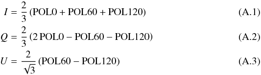 where POL0, POL60, and POL120 are the images of RS Pup in the three polarizers, after the PSF wings and sky background were subtracted. The degree of linear polarization pL was then derived through
 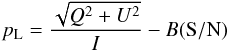 (A.4)where B(S / N) is the bias correction depending on the photometric S/N as listed in Table A.1 of Sparks & Axon (1999). The polarization electric-vector position angle in detector coordinates θD was derived through the expression:
 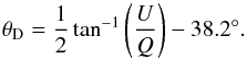 (A.5)The uncertainties were propagated to the Stokes parameters starting from the photometric error bars produced by the ACS processing pipeline σ(POL0), σ(POL60), and σ(POL120) through
 ![Mathematical equation: \appendix \setcounter{section}{1} \begin{eqnarray} \label{EqErrI} \sigma^2(I) &=& \left( 2/3 \right)^2 \left[ \sigma^2(\mathrm{POL0}) + \sigma^2(\mathrm{POL60}) + \sigma^2(\mathrm{POL120}) \right] \\[3mm] \label{EqErrQ} \sigma^2(Q)& =& \left( 2/3 \right)^2 \left[ 4\,\sigma^2(\mathrm{POL0}) + \sigma^2(\mathrm{POL60}) + \sigma^2(\mathrm{POL120}) \right] \\[3mm] \label{EqErrU} \sigma^2(U)& =& \left(4/3 \right) \left[ \sigma^2(\mathrm{POL60}) + \sigma^2(\mathrm{POL120}) \right], \end{eqnarray}](/articles/aa/full_html/2014/12/aa24395-14/aa24395-14-eq231.png) and to the degree of linear polarization pL through
and to the degree of linear polarization pL through ![Mathematical equation: \appendix \setcounter{section}{1} \begin{eqnarray} \label{EqVarUI} \sigma^2(U/I) &=& \frac{U^2}{I^2} \ \left( \frac{\sigma^2(U)}{U^2} + \frac{\sigma^2(I)}{I^2} - \frac{\sigma^4(I)}{I^4} \right) \\[3mm] \label{EqVarQI} \sigma^2(Q/I) &= &\frac{Q^2}{I^2} \ \left( \frac{\sigma^2(Q)}{Q^2} + \frac{\sigma^2(I)}{I^2} - \frac{\sigma^4(I)}{I^4} \right) \\[3mm] \label{EqVarPL} \sigma^2(p_{\rm L}) &= \frac{\sigma^2(U)\ \sigma^2(U/I) + \sigma^2(Q)\ \sigma^2(Q/I)}{(Q + U)^2} \cdot \end{eqnarray}](/articles/aa/full_html/2014/12/aa24395-14/aa24395-14-eq232.png)
An animated video sequence showing the propagation of the light echoes of RS Pup can be downloaded from http://hubblesite.org/newscenter/archive/releases/star/2013/51/
Data available from https://www.astro.princeton.edu/~draine/dust/scat.html
A ground-based imaging survey by one of us (H.E.B., in prep.) of ~100 Galactic Cepheids failed to reveal any new associated reflection nebulae.
Acknowledgments
We thank Dr Daniel Rouan for fruitful discussions of the determination of the geometry of RS Pup’s nebula. We acknowledge financial support from the “Programme National de Physique Stellaire” (PNPS) of CNRS/INSU, France. Support for Program number GO-13454 was provided by NASA through a grant from the Space Telescope Science Institute, which is operated by the Association of Universities for Research in Astronomy, Incorporated, under NASA contract NAS5-26555. P.K. and A.G. acknowledge support of the French-Chilean exchange program ECOS-Sud/CONICYT. L.Sz. acknowledges support from the ESTEC Contract No. 4000106398/12/NL/KML. A.G. acknowledges support from FONDECYT grant 3130361. This research received the support of PHASE, the high angular resolution partnership between ONERA, Observatoire de Paris, CNRS, and University Denis Diderot Paris 7. We used the SIMBAD and VIZIER databases at the CDS, Strasbourg (France), and NASA’s Astrophysics Data System Bibliographic Services. We used the IRAF package, distributed by the NOAO, which are operated by the Association of Universities for Research in Astronomy, Inc., under cooperative agreement with the National Science Foundation. Some of the data presented in this paper were obtained from the Multimission Archive at the Space Telescope Science Institute (MAST). STScI is operated by the Association of Universities for Research in Astronomy, Inc., under NASA contract NAS5-26555. Support for MAST for non-HST data is provided by the NASA Office of Space Science via grant NAG5-7584 and by other grants and contracts.
References
- Afşar, M., & Bond, H. E. 2007, AJ, 133, 387 [NASA ADS] [CrossRef] [Google Scholar]
- Anderson, R. I. 2014, A&A, 566, L10 [NASA ADS] [CrossRef] [EDP Sciences] [Google Scholar]
- Anderson, R. I., Ekström, S., Georgy, C., et al. 2014, A&A, 564, A100 [NASA ADS] [CrossRef] [EDP Sciences] [Google Scholar]
- Barmby, P., Marengo, M., Evans, N. R., et al. 2011, AJ, 141, 42 [NASA ADS] [CrossRef] [Google Scholar]
- Barnes, III, T. G., Jefferys, W. H., Berger, J. O., et al. 2003, ApJ, 592, 539 [NASA ADS] [CrossRef] [Google Scholar]
- Barnes, III, T. G., Storm, J., Jefferys, W. H., Gieren, W. P., & Fouqué, P. 2005, ApJ, 631, 572 [NASA ADS] [CrossRef] [Google Scholar]
- Benedict, G. F., McArthur, B. E., Feast, M. W., et al. 2007, AJ, 133, 1810 [NASA ADS] [CrossRef] [Google Scholar]
- Bennett, C. L., Larson, D., Weiland, J. L., & Hinshaw, G. 2014, ApJ, 794, 135 [NASA ADS] [CrossRef] [Google Scholar]
- Berdnikov, L. N., Henden, A. A., Turner, D. G., & Pastukhova, E. N. 2009, Astron. Lett., 35, 406 [NASA ADS] [CrossRef] [Google Scholar]
- Biretta, J., Kozhurina-Platais, V., Boffi, F., Sparks, W., & Walsh, J. 2004, ACS Polarization Calibration – I. Introduction and Status Report, Tech. Rep. (STScI) [Google Scholar]
- Bond, H. E., & Sparks, W. B. 2009, A&A, 495, 371 [NASA ADS] [CrossRef] [EDP Sciences] [Google Scholar]
- Couderc, P. 1939, Annales d’Astrophysique, 2, 271 [Google Scholar]
- Cracraft, M., & Sparks, W. B. 2007, ACS Polarization Calibration – Data, Throughput, and Multidrizzle Weighting Schemes, Tech. Rep. (STScI) [Google Scholar]
- Di Benedetto, G. P. 1997, ApJ, 486, 60 [NASA ADS] [CrossRef] [Google Scholar]
- Draine, B. T. 2003, ApJ, 598, 1017 [NASA ADS] [CrossRef] [Google Scholar]
- Fouqué, P., Storm, J., & Gieren, W. 2003, in Stellar Candles for the Extragalactic Distance Scale, eds. D. Alloin, & W. Gieren (Berlin: Springer Verlag), Lect. Notes Phys., 635, 21 [Google Scholar]
- Fouqué, P., Arriagada, P., Storm, J., et al. 2007, A&A, 476, 73 [NASA ADS] [CrossRef] [EDP Sciences] [Google Scholar]
- Freedman, W. L., & Madore, B. F. 2010, ARA&A, 48, 673 [NASA ADS] [CrossRef] [Google Scholar]
- Freedman, W. L., Madore, B. F., Gibson, B. K., et al. 2001, ApJ, 553, 47 [NASA ADS] [CrossRef] [Google Scholar]
- Gieren, W. P., Barnes, III, T. G., & Moffett, T. J. 1993, ApJ, 418, 135 [NASA ADS] [CrossRef] [Google Scholar]
- Gonzaga, S., Hack, W., Fruchter, A., & Mack, J. 2012, The DrizzlePac Handbook (STScI) [Google Scholar]
- Graham, J. R., Kalas, P. G., & Matthews, B. C. 2007, ApJ, 654, 595 [NASA ADS] [CrossRef] [Google Scholar]
- Groenewegen, M. A. T. 2008, A&A, 488, 25 [NASA ADS] [CrossRef] [EDP Sciences] [Google Scholar]
- Groenewegen, M. A. T. 2013, A&A, 550, A70 [NASA ADS] [CrossRef] [EDP Sciences] [Google Scholar]
- Havlen, R. J. 1972, A&A, 16, 252 [NASA ADS] [Google Scholar]
- Henyey, L. G., & Greenstein, J. L. 1940, Annales d’Astrophysique, 3, 117 [NASA ADS] [Google Scholar]
- Henyey, L. G., & Greenstein, J. L. 1941, ApJ, 93, 70 [NASA ADS] [CrossRef] [Google Scholar]
- Hindsley, R., & Bell, R. A. 1986, PASP, 98, 881 [NASA ADS] [CrossRef] [Google Scholar]
- Hindsley, R. B., & Bell, R. A. 1989, ApJ, 341, 1004 [NASA ADS] [CrossRef] [Google Scholar]
- Jones, T. J., Humphreys, R. M., Helton, L. A., Gui, C., & Huang, X. 2007, AJ, 133, 2730 [NASA ADS] [CrossRef] [Google Scholar]
- Kervella, P., Mérand, A., Szabados, L., et al. 2008, A&A, 480, 167 [NASA ADS] [CrossRef] [EDP Sciences] [Google Scholar]
- Kervella, P., Mérand, A., Szabados, L., et al. 2012, A&A, 541, A18 [NASA ADS] [CrossRef] [EDP Sciences] [Google Scholar]
- Madore, B. F., & Freedman, W. L. 2012, ApJ, 744, 132 [NASA ADS] [CrossRef] [Google Scholar]
- Marengo, M., Evans, N. R., Barmby, P., et al. 2010, ApJ, 725, 2392 [NASA ADS] [CrossRef] [Google Scholar]
- Mérand, A., Kervella, P., Coudé du Foresto, V., et al. 2005, A&A, 438, L9 [Google Scholar]
- Nardetto, N., Mourard, D., Mathias, P., Fokin, A., & Gillet, D. 2007, A&A, 471, 661 [NASA ADS] [CrossRef] [EDP Sciences] [Google Scholar]
- Nardetto, N., Storm, J., Gieren, W., Pietrzyński, G., & Poretti, E. 2014, in IAU Symp. 301, eds. J. A. Guzik, W. J. Chaplin, G. Handler, & A. Pigulski, 145 [Google Scholar]
- Perryman, M. A. C., & ESA 1997, in The Hipparcos and TYCHO catalogues, Astrometric and photometric star catalogues derived from the ESA Hipparcos Space Astrometry Mission, ESA SP, 1200 [Google Scholar]
- Pickles, A., & Depagne, É. 2010, PASP, 122, 1437 [NASA ADS] [CrossRef] [Google Scholar]
- Pilecki, B., Graczyk, D., Pietrzyński, G., et al. 2013, MNRAS, 436, 953 [NASA ADS] [CrossRef] [Google Scholar]
- Riess, A. G., Macri, L., Li, W., et al. 2009, ApJS, 183, 109 [NASA ADS] [CrossRef] [Google Scholar]
- Riess, A. G., Macri, L., Casertano, S., et al. 2011, ApJ, 730, 119 [NASA ADS] [CrossRef] [Google Scholar]
- Riess, A. G., Casertano, S., Anderson, J., MacKenty, J., & Filippenko, A. V. 2014, ApJ, 785, 161 [NASA ADS] [CrossRef] [Google Scholar]
- Sahai, R., Zijlstra, A., Bujarrabal, V., & te Lintel Hekkert, P. 1999, AJ, 117, 1408 [NASA ADS] [CrossRef] [Google Scholar]
- Sandage, A., Tammann, G. A., Saha, A., et al. 2006, ApJ, 653, 843 [NASA ADS] [CrossRef] [Google Scholar]
- Schulte-Ladbeck, R. E., Pasquali, A., Clampin, M., et al. 1999, AJ, 118, 1320 [NASA ADS] [CrossRef] [Google Scholar]
- Shen, Y., Draine, B. T., & Johnson, E. T. 2009, ApJ, 696, 2126 [NASA ADS] [CrossRef] [Google Scholar]
- Sparks, W. B. 1994, ApJ, 433, 19 [NASA ADS] [CrossRef] [Google Scholar]
- Sparks, W. B., & Axon, D. J. 1999, PASP, 111, 1298 [Google Scholar]
- Sparks, W. B., Bond, H. E., Cracraft, M., et al. 2008, AJ, 135, 605 [NASA ADS] [CrossRef] [Google Scholar]
- Sterken, C. 2005, in The Light-Time Effect in Astrophysics: Causes and cures of the O-C diagram, ed. C. Sterken, ASP Conf. Ser., 335, 3 [Google Scholar]
- Storm, J., Carney, B. W., Gieren, W. P., et al. 2004, A&A, 415, 531 [NASA ADS] [CrossRef] [EDP Sciences] [Google Scholar]
- Storm, J., Gieren, W., Fouqué, P., et al. 2011, A&A, 534, A94 [NASA ADS] [CrossRef] [EDP Sciences] [Google Scholar]
- Sugerman, B. E. K. 2003, AJ, 126, 1939 [NASA ADS] [CrossRef] [Google Scholar]
- Tammann, G. A., Sandage, A., & Reindl, B. 2003, A&A, 404, 423 [NASA ADS] [CrossRef] [EDP Sciences] [Google Scholar]
- Turner, D. G., Majaess, D. J., Lane, D. J., et al. 2012, MNRAS, 422, 2501 [NASA ADS] [CrossRef] [Google Scholar]
- Tylenda, R., & Kamiński, T. 2012, A&A, 548, A23 [NASA ADS] [CrossRef] [EDP Sciences] [Google Scholar]
- Ubeda, L. et al. 2012, Advanced Camera for Surveys Instrument Handbook for Cycle 21 v. 12.0 (Baltimore: STScI) [Google Scholar]
- van Leeuwen, F. 2007, A&A, 474, 653 [NASA ADS] [CrossRef] [EDP Sciences] [Google Scholar]
- van Leeuwen, F., Feast, M. W., Whitelock, P. A., & Laney, C. D. 2007, MNRAS, 379, 723 [NASA ADS] [CrossRef] [Google Scholar]
- Volten, H., Muñoz, O., Hovenier, J. W., et al. 2007, A&A, 470, 377 [NASA ADS] [CrossRef] [EDP Sciences] [Google Scholar]
- Westerlund, B. 1961, PASP, 73, 72 [NASA ADS] [CrossRef] [Google Scholar]
- White, R. L. 1979, ApJ, 229, 954 [NASA ADS] [CrossRef] [Google Scholar]
- Windmark, F., Lindegren, L., & Hobbs, D. 2011, A&A, 530, A76 [NASA ADS] [CrossRef] [EDP Sciences] [Google Scholar]
All Tables
Observationally determined distances of RS Pup (“IRSB” stands for “infrared surface brightness”).
All Figures
|
Fig. 1 Image of the PSF star HD 68111 (PSF-Blue) in the F606W+POL0V polarizing filter setup (left) and the derived composite synthetic PSF (right). |
| In the text | |
|
Fig. 2 First observing epoch of RS Pup before (left) and after (right) the subtraction of the PSF wings and sky background, with the same gray scale (proportional to the square root of the flux count). The “double doughnut” feature in the lower left quadrant of the image is an optical artifact. |
| In the text | |
|
Fig. 3 Average maps of the Stokes I (left, in e− s-1) and degree of linear polarization pL (right), computed over the seven observing epochs of RS Pup (north is up and east to the left). |
| In the text | |
|
Fig. 4 Synthetic light curve of RS Pup (blue curve) in the F606W filter with the ACS photometry derived from the ghost image of the telescope pupil (open circles) phased with T0 = 2 455 252.64 (JD⊙) and P = 41.5117 days. |
| In the text | |
|
Fig. 5 Maps of the average flux f0 (left panel, in e− s-1), amplitude A (central panel, in e− s-1), and phase offset Δφ (right panel) of the photometric variations observed in the southern quadrant of the nebula of RS Pup. The FoV is 68.3′′ × 68.3′′, with north up and east to the left. |
| In the text | |
|
Fig. 6 Geometry of the light echoes in the dust surrounding RS Pup. |
| In the text | |
|
Fig. 7 Median pL values observed in the nebula of RS Pup in 1% bins as a function of the percentile of highest values. The attached vertical segments show the full range of values of pL in each bin. The orange segment on the vertical axis shows the adopted uncertainty range for pmax = 51.5% ± 2.0%. |
| In the text | |
|
Fig. 8 Map of the degree of linear polarization pL in the nebula of RS Pup from VLT/FORS observations (Kervella et al. 2012). |
| In the text | |
|
Fig. 9 Milky Way dust (pmax = 51.5%, solid black curve) and Rayleigh (pmax = 51.5%, θmax = 92°, dashed curve) models of the linear polarization degree pL(θ). The observed polarization function measured by Sparks et al. (2008) for the dust surrounding V838 Mon is shown as a blue curve. |
| In the text | |
|
Fig. 10 Color composite view of the circumstellar nebula of RS Pup assembled from the ACS WFC images in the F435W and F606W filters obtained on 2010 March 26 (color rendition: NASA, ESA, Z. Levay, and the Hubble Heritage Team STScI/AURA-Hubble/Europe Collaboration). The maximum light echoes are visible as blue rings owing to the hotter temperature of the central star around its maximum light. North is up and east to the left, and the FoV is 2.9 × 2.9 arcmin. |
| In the text | |
|
Fig. 11 Map of the polarized flux I × pL in the nebula of RS Pup (in e− s-1). The red contours enclose the regions that were selected for the distance fit. The artifacts and background stars have been masked, and the yellow cross marks the position of RS Pup. The dashed yellow circles mark 30′′ and 60′′ angular separations from the Cepheid, and the FoV is 68.3′′ × 68.3′′ with north up and east to the left. |
| In the text | |
|
Fig. 12 Map of the reduced χ2 of RS Pup’s distance adjustment for the scaled Milky Way dust polarization model (left panel) and the scaled Rayleigh scattering polarization model with θmax = 92° (right panel), as a function of the adopted pmax value (vertical axis). The white rectangle indicates horizontally the distance range found in the literature and vertically the adopted pmax uncertainty range (51.5% ± 2.0%). The white dots show the position of the minimum χ2 for pmax = 49.5, 51.5 and 53.5%. The color scale shown above the map is a function of the square root of the reduced χ2 value. |
| In the text | |
|
Fig. 13 Reduced χ2 curve of the distance fit for the scaled Milky Way dust polarization model with pmax = 49.5%, 51.5%, and 53.5%. |
| In the text | |
|
Fig. 14 Period–luminosity diagram in the V band showing the position of RS Pup. The relations by Fouqué et al. (2007) and Benedict et al. (2007) are shown as solid and dashed lines, respectively. |
| In the text | |
Current usage metrics show cumulative count of Article Views (full-text article views including HTML views, PDF and ePub downloads, according to the available data) and Abstracts Views on Vision4Press platform.
Data correspond to usage on the plateform after 2015. The current usage metrics is available 48-96 hours after online publication and is updated daily on week days.
Initial download of the metrics may take a while.