| Issue |
A&A
Volume 571, November 2014
|
|
|---|---|---|
| Article Number | A77 | |
| Number of page(s) | 8 | |
| Section | Numerical methods and codes | |
| DOI | https://doi.org/10.1051/0004-6361/201424237 | |
| Published online | 14 November 2014 | |
A semianalytical light curve model and its application to type IIP supernovae
1 Department of Optics and Quantum Electronics, University of Szeged, 6720 Szeged, Hungary
e-mail: This email address is being protected from spambots. You need JavaScript enabled to view it.
2 Department of Astronomy, University of Texas at Austin, Austin, TX, USA
Received: 19 May 2014
Accepted: 15 September 2014
Abstract
The aim of this work is to present a semianalytical light curve model code that can be used for estimating physical properties of core collapse supernovae (SNe) in a quick and efficient way. To verify our code we fit light curves of Type II SNe and compare our best parameter estimates to those from hydrodynamical calculations. For this analysis, we use quasi-bolometric light curves of five different Type IIP SNe. In each case, we obtain appropriate results for initial pre-supernova parameters. We conclude that this semianalytical light curve model is useful to obtaining approximate physical properties of Type II SNe without using time-consuming numerical hydrodynamic simulations.
Key words: supernovae: general
© ESO, 2014
1. Introduction
The light curves of Type IIP supernovae (SNe) are characterized by a plateau phase with a duration of about 80–120 days and a quasi-exponential tail caused by the radioactive decay of 56Co (e.g., Maguire et al. 2010). The emitted flux at later phases is directly determined by the mass of ejected 56Ni. Besides nickel mass, other parameters specify the bolometric luminosity of SNe, such as explosion energy, ejected mass, and the initial size of the radiating surface (Grassberg et al. 1971; Litvinova & Nadyozhin 1985). The radius of this surface is thought to be equal to the radius of the progenitor at the moment of shock breakout following core collapse.
A general approach to determine the properties of supernova explosions is the modeling of observed data with hydrodynamical codes (Grassberg et al. 1971; Falk & Arnett 1977; Hillebrandt & Müller 1981; Blinnikov et al. 2000; Nadyozhin 2003; Utrobin et al. 2007; Pumo et al. 2010; Bersten et al. 2011). However, a simple analytical method may also be used to obtain approximate results (Arnett 1980, 1982; Zampieri et al. 2003; Chatzopoulos et al. 2012). With the help of these analytic light curve models, the basic physical parameters, such as explosion energy, ejected mass and initial radius, can be estimated (Arnett 1980; Popov 1993). Although such simple estimates can be considered only preliminary, they can be obtained without running complicated, time-consuming hydrodynamical simulations. Analytic codes may be useful in providing constraints for the most important physical parameters, which can be used as input in more detailed simulations. Also, analytic codes may also give first-order approximations when observational information is limited, for example, when only photometry and no spectroscopy is available for a particular SN.
In this paper we describe a semianalytical light curve model, which is based on the model originally developed by Arnett & Fu (1989). We assume a homologously expanding and spherically symmetric SN ejecta have a uniform density core and an exponential density profile in the other layers. Radiation transport is treated by the diffusion approximation. The effect of recombination causing the rapid change of the effective opacity in the envelope is taken into account in a simple form introduced by Arnett & Fu (1989).
This paper is organized as follows: in Sect. 2, we describe the model and its implementation, and also present the effect of variations of the initial input parameters on the calculated bolometric luminosity. In Sect. 3, we compare the results obtained for SN 2004et, SN 2005cs, SN 2009N, SN 2012A, and SN 2012aw from our code and several hydrodynamic computations. Finally, Sect. 4 summarizes the main results of this paper.
2. Main assumptions and model parameters
2.1. The light curve model
We adopt the radiative diffusion model originally developed by Arnett (1980) and modified by Arnett & Fu (1989) to take the effect of the recombination front in the ejecta into account. Below we review the original derivation, and present some corrections and implementations for numerical computations.
The first law of thermodynamics in Lagrangian coordinates for a spherical star may be written as  (1)where E is the internal energy per unit mass, P is the pressure, V = 1 /ρ is the specific volume, ϵ is the entire energy production rate per unit mass, and L is the luminosity (Arnett 1980, 1982). In a radiation-dominated envelope, the internal energy per unit mass is E = aT4V and the pressure is P = E/ 3V, where a is the radiation density constant. The energy loss is driven by photon diffusion, so we may use the following equation for the derivative of the luminosity:
  (2)where κ is the mean opacity, T is the temperature, and ρ is the density. Since the supernova ejecta expand homologously we define a comoving, dimensionless radius x as
  (3)where r is the distance of a particular layer from the center and R(t) is the total radius of the expanding envelope at a given time. In the comoving coordinate system, we are able to separate the time and space dependence of the physical properties. Thus, the density profile can be described as
  (4)where R0 is the initial radius and η(x) ~ exp(−αx) where α is assumed to be a small positive integer. The time-dependent term describes the dilution of the density due to expansion.
The ejecta are expected to be fully ionized shortly after the explosion, so it seems reasonable to consider a recombination front that moves inward through the envelope. The assumed recombination wave divides the ejecta into two different parts. The boundary separating the two layers occurs at the dimensionless radius xi where the local temperature T(x) drops below the recombination temperature Trec. Inside this recombination radius, the ejecta are assumed to be fully ionized. The opacity (κ) changes strongly at the boundary layer separating the two parts. Because the opacity has a strong nonlinear dependence on the temperature, we assume a simple step-function to approximate its behavior (Arnett & Fu 1989):  (5)where Trec is the recombination temperature, below which the ejecta are mostly neutral. In this approximation, we use the Thomson-scattering opacity for pure hydrogen gas as κ ~ 0.4 cm2/g, and model the presence of heavier elements by setting κ to lower values. For example, κ ~ 0.2 cm2/g is assumed for a He-dominated ejecta, while for a He-burned atmosphere κ may be ~0.1 cm2/g.
Following Arnett (1980), the temperature evolution and its spatial profile can be approximated as  (6)and the radial components of this function is
  (7)which does not change during the expansion. While implementing the temperature profile in our C-code, we found that the direct application of the sin(x) function caused numerical instabilities due to rounding errors around x ≈ 1. To reduce this problem, we used a 4th order Taylor-series expansion of the ψ(x) function (see Fig. 1). The implementation of the Taylor-series approximation increased the numerical stability when computing the effect of recombination.
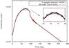 |
Fig. 1 Model light curve computed with exact sin(πx)/(πx) temperature profile (black) and with 4th order Taylor series (red). |
Another important physical quantity is the energy production rate, which can be defined as  (8)In this case, a central energy production is assumed, which means that ξ(x) is the Dirac-delta function at x = 0. The temporal dependence of the ϵ(t) function was specified by assuming either radioactive decay or magnetar-controlled energy input. In the following subsections we summarize these two different conditions.
2.1.1. Radioactive energy input
In this case only the radioactive decay of 56Ni and 56Co supplies the input energy. In such a model ϵ(0,0) is equal to the initial energy production rate of 56Ni-decay. The time-dependent part of the ϵ(x,t) function, when the ejecta are optically thick for gamma-rays, is given by  (9)where XNi and XCo are the number of nickel and cobalt atoms per unit mass, respectively, ϵNi and ϵCo are the energy production rate from the decay of these elements. The number of the radioactive elements varies as
  (10)where z = t/τNi is the dimensionless timescale of the Ni-Co decay, τNi and τCo are the decay time of nickel and cobalt, respectively.
The comoving coordinate of the recombination front is denoted as xi. Following Arnett & Fu (1989) it is assumed that the radiative diffusion takes place only within xi where κ> 0, and the photons freely escape from x = xi. Thus, the surface at xi acts as a pseudo-photosphere.
After inserting the quantities defined above into Eq. (1), we have  (11)Now, applying the assumption made by (Arnett 1982, see his Eq. (13)), the temporal and spatial parts of Eq. (11) can be separated, thus, both of them are equal to a constant (the “eigenvalue” of the solution). After separation, the equation describing the temporal evolution of the φ(t) function can be expressed as
 ![Mathematical equation: \begin{eqnarray} \frac{{\rm d}\phi(t)}{{\rm d}t}\ \tau_{\rm Ni}\!=\!\frac{R(t)}{R_0\ x_i^3}\!\left[p_1 \zeta(t) \!-\! p_2\ x_i\ \phi(t) \!-\! 2\ \tau_{\rm Ni}\ x_i^2\ \phi(t) \!\frac{R_0}{R(t)}\! \frac{{\rm d}x_i}{{\rm d}t}\right],\, \end{eqnarray}](/articles/aa/full_html/2014/11/aa24237-14/aa24237-14-eq56.png) (12)where we corrected a misprint that occurred in Eq. (A41) of Arnett & Fu (1989). This equation contains two parameters defined as
(12)where we corrected a misprint that occurred in Eq. (A41) of Arnett & Fu (1989). This equation contains two parameters defined as  (13)
where
(13)
where
 and
and
 are the initial total nickel mass and the initial thermal energy, respectively.
Equation (12) was solved by the Runge-Kutta method with the approximation of dxi/ dt ≈ Δxi/ Δt, where a small time-step of Δt = 1 s was applied. In the nth time-step  was used, where
  and
and  are the dimensionless radii of the recombination layer in the nth and (n − 1)th time-step, respectively. To determine the value of in every time-step, our code divides the envelope into thin (δx = 10-9) layers, then calculates the temperature in each layer starting from the outmost layer at x = 1 until the temperature exceeds the recombination temperature Trec. If that occurs at the kth layer then xi ≈ (xk + δx/ 2) is chosen as the new radius of the recombination layer.
Finally, the total bolometric luminosity can be expressed as a sum of the radioactive heating plus the energy released by the recombination:  (14)where
  is the diffusion timescale, and Q = 1.6 × 10¹³(Z/A)Z4/3 is the recombination energy per unit mass. The effect of gamma-ray leakage can be taken into account as
  (15)where the Ag factor refers to the effectiveness of gamma-ray trapping. The optical depth of gamma rays can be defined as τg = Ag/t2 (Chatzopoulos et al. 2012). This parameter is significant in modeling the light curves of Type IIb and Ib/c SNe.
2.1.2. Magnetar spin-down
Magnetars represent a subgroup of neutron stars with a strong (1014 − 1015 G) magnetic field. The spin-down power of a newly formed magnetar can create a brighter and faster evolving SN light curve than radioactive decay (Piro & Ott 2011). This mechanism can contribute to the extreme peak luminosity of Type Ib/c and super-luminous SNe (Woosley 2010; Kasen & Bildsten 2010; Chatzopoulos et al. 2012).
In this case, ϵ(t) includes radioactive energy production as well as magnetar spin-down:  (16)where ϵNi(t) is the energy production rate of radioactive decay of nickel and cobalt as defined in the previous section and ϵM(t) is the energy production rate of the spin-down per unit mass. The power source of the magnetar is given by the spin-down formula
  (17)where Mej is the ejected mass, Ep is the initial rotational energy of the magnetar, tp is the characteristic timescale of spin-down, which depends on the strength of the magnetic field, and l = 2 for a magnetic dipole.
Solving Eq. (1) as in the previous section the φ(t) function can be expressed as ![Mathematical equation: \begin{eqnarray} \frac{{\rm d}\phi(t)}{{\rm d}t}\ \tau_{\rm Ni} & = & \frac{R(t)}{R_0\ x_i^3}\left[p_1 \zeta(t) - p_2\ x_i\ \phi(t)\ +\ p_3 \frac{1}{(1 + t/t_{\rm p})^2} \right] \nonumber \\ & & - 2 \tau_{\rm Ni}\ \phi(t)\ \frac{1}{x_i} \frac{{\rm d}x_i}{{\rm d}t}, \end{eqnarray}](/articles/aa/full_html/2014/11/aa24237-14/aa24237-14-eq86.png) (18)where p3 = τNiEp/ETh(0)tp. The total bolometric luminosity in this configuration is calculated using Eqs. (14), (15) with the numerical integration of the modified φ(t) function.
(18)where p3 = τNiEp/ETh(0)tp. The total bolometric luminosity in this configuration is calculated using Eqs. (14), (15) with the numerical integration of the modified φ(t) function.
To verify the magnetar model, we compared our results with the estimated peak luminosities defined by Kasen & Bildsten (2010): ![Mathematical equation: \begin{eqnarray} L_{\rm peak}^{\rm ref} \approx \frac{E_{\rm p}\ t_{\rm p}}{t_{\rm d}^2}\ \left[\ln\left(1+\frac{t_{\rm d}}{t_{\rm p}}\right)-\frac{t_{\rm d}}{t_{\rm d} + t_{\rm p}}\right], \end{eqnarray}](/articles/aa/full_html/2014/11/aa24237-14/aa24237-14-eq88.png) (19)where td is the effective diffusion timescale (Arnett 1980):
(19)where td is the effective diffusion timescale (Arnett 1980):  (20)and
 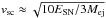 is the characteristic ejecta velocity.
For the test case, we used the following fixed parameters: R0 = 5 × 1011 cm; Mej = 1 M⊙;  ; Trec = 0 K (i.e., no recombination); Ekin(0) = 3 foe (1 foe = 1051 erg); ETh(0) = 2 foe; α = 0 (constant density model); κ = 0.34cm2/ g; Ag = 106 day2 (full gamma-ray trapping). These parameters imply vsc ~ 22 400 km s-1 and td ~ 14 days. Values of Ep and tp were varied within a range typical for magnetars (Kasen & Bildsten 2010). Table 1 shows the peak luminosities estimated from the formulae above (
 ) and provided by our code (
 ). We found acceptable agreement between the calculated and the model values, although the analytic formula slightly underestimates the model peaks.
Comparison of magnetar model peak luminosities with the analytic estimates.
2.2. The effect of varying input parameters
To create light curves we need to integrate Eqs. (12)–(18) then apply Eqs. (14), (15) in every time-step. The input parameters for the model are the following:
-
R0: initial radius of the ejecta (in 1013 cm);
-
Mej: ejected mass (in M⊙);
-
 : initial nickel mass (in M⊙);
 -
Trec: recombination temperature (in K);
-
Ekin(0): initial kinetic energy (in foe);
-
ETh(0): initial thermal energy (in foe);
-
α: density profile exponent ;
-
κ: opacity (in cm2/ g);
-
Ep: initial rotational energy of the magnetar (in foe);
-
tp: timescale of magnetar spin-down (in day); and
-
Ag: gamma-ray leakage exponent (in day2).
We tested our code by changing these input parameters and comparing the resulting light curves to those of Arnett & Fu (1989). The parameters were varied one by one using three different values while holding the others constant. The following reference parameters were chosen (plotted with black): R0 = 5 × 1012 cm; Mej = 10 M⊙;  ; Trec = 6000 K; Ekin(0) = 1 foe; ETh(0) = 1 foe; α = 0; κ = 0.3 cm2/ g; Ep = 0 foe; tp = 0 days; Ag = 106 day2. When the magnetar energy input was taken into account the two characteristic parameters were Ep = 1 foe and tp = 10 days.
First, we created light curves with three different radii: 5 × 10¹¹, 5 × 10¹², and 5 × 1013 cm. As seen in Fig. 2a, the modification of this parameter mainly influences the early part of the light curve. As a result of the increasing radius, the peak of the light curve becomes wider and flatter. The rapid decline after the plateau also becomes steeper. As Type IIP SNe exhibit steep declines after the plateau phase, this behavior is consistent with their larger progenitor radii. Our code replicates this behavior.
Next, we set 5, 10, and 15 M⊙ as the three input values of the ejected mass. This parameter also affects the maximum and the width of the light curve (Fig. 2b). Higher ejecta masses result in lower peak luminosities and more extended plateau phases.
The three different values of nickel mass were 0.001, 0.01, and 0.1 M⊙. Figure 2c shows the strong influence of this parameter on all phases of the light curve. Increasing nickel mass causes a global increase of the luminosity at all phases, as expected. This panel also illustrates that the late-phase luminosity level depends on only the Ni-mass in the case of full gamma-ray trapping.
Figure 2d shows the effect of the modification of the recombination temperature from 5000 K to 7000 K. This parameter has no major influence on the light curve. Higher Trec results in a shorter plateau phase and the short decline phase after the plateau also becomes steeper. The recombination temperature is the parameter that can be used to take the ejecta chemical composition into account. For example, the recombination temperature for pure H ejecta is ~5000 K, but for He-dominated ejecta it is higher, Trec ~ 7000 K (Grassberg & Nadyozhin 1976), or Trec ~ 10 000 K (Hatano et al. 1999).
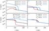 |
Fig. 2 Effect of changing the initial radius of the ejecta (panel a)), the ejected mass (panel b)), the initial nickel mass (panel c)), and the recombination temperature (panel d)). |
One of the most important parameters of SN events is the explosion energy (ESN), which is the sum of the kinetic and the thermal energy. In this work, we examined the effect of these two parameters separately. The three values of the kinetic energy were 0.5, 1, and 5 foe. As Fig. 3a shows, this parameter has significant influence on the shape of the early light curve, but does not have any effect on the late part because, again, the luminosity at late phases are set by only the initial Ni-mass. When the kinetic energy is lower, the plateau becomes wider, while the maximum luminosity decreases. Note that using extremely high kinetic energy results in the lack of the plateau phase. The influence of the thermal energy is somewhat similar: it mainly affects the early light curve (Fig. 3b). Increasing thermal energy widens the plateau, and the peak luminosity rises. For high ETh the plateau phase starts to disappear, just as for high Ekin.
The density profile exponent was chosen as 0, 1, and 2. Figure 3c. shows that the different values cause changes mainly in the maximum of the light curve and the duration of the plateau phase. If the density profile exponent is higher, then the luminosity is reduced and the peak becomes wider.
Next, we examined the effect of changing opacity (Fig. 3d). The chosen values of this parameter were 0.2, 0.3, and 0.4 cm2/ g. Decreasing opacity results in rising luminosity and shorter plateau phase.
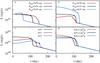 |
Fig. 3 Effect of changing the initial kinetic energy (panel a)), the initial thermal energy (panel b)), the density profile exponent (panel c)), and the opacity (panel d)). |
To test the magnetar energy input, the initial rotational energy of the magnetar were set as 0.01, 0.1, and 1 foe. As Fig. 4a shows, this parameter has significant influence on the entire light curve. Higher Ep results in rising luminosities and broader plateau phase. If the initial rotational energy is not comparable to the recombination energy, no recognizable plateau phase is created by the magnetar energy input.
The characteristic timescale of the spin-down was chosen as tp = 10, 100, and 500 days. The light curve strongly depends on the ratio of the effective diffusion time and spin-down timescale (Fig. 4b). As far as tp is well below td, increasing spin-down time causes higher luminosities and wider plateau phase, but if tp ≫ td, the maximum starts to decrease. In this particular case td ~ 97.35 days was applied.
Finally, the gamma-ray leakage exponent was varied as 104, 5 × 10⁴, and 106 day2. Figure 4c shows the strong influence of this parameter on the entire light curve. The tail luminosity is significantly related to the gamma-ray leakage, as expected. Increasing Ag results in a wider plateau phase, and also increases the tail luminosity.
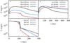 |
Fig. 4 Effect of changing the initial rotation energy of the magnetar (panel a)), the characteristic timescale of magnetar spin-down (panel b)), the gamma-ray leakage exponent (panel c)). |
To summarize the results of these tests, we conclude that:
-
a)
the duration of the plateau phase is strongly influencedby the values of the initial radius of the ejecta, theejected mass, the density profile exponent, and the kinetic energy;
-
b)
the opacity, the initial nickel mass, and the recombination temperature are weakly correlated with the duration of the plateau;
-
c)
the maximum brightness and the form of the peak mainly depend on the thermal energy, the initial nickel mass, the initial radius of the ejecta, the density profile exponent, and the magnetar input parameters;
-
d)
the peak luminosity of the plateau is weakly influenced by the ejected mass and the opacity;
-
e)
the late light curve is determined by the amount of the initial nickel mass, the gamma-ray leakage exponent, and the characteristic features of the magnetar; and
-
f)
the light curve is less sensitive to the recombination temperature and opacity.
These results are generally in very good agreement with the conclusions by Arnett & Fu (1989) regarding the behavior of the initial radius, the recombination temperature and the factor 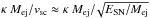 . Furthermore, our results show the same parameter dependence of the plateau duration as calculated by Popov (1993).
2.3. Parameter correlations
The correlation between parameters as examined by the Pearson correlation coefficient method, which measures the linear correlation between two variables. For this comparison, we first synthesized a test light curve for both the radioactive decay and magnetar-controlled energy input models. Then, we tried each parameter-combination to create the same light curve and determine the correlations among the parameters. The scatter diagrams (Fig. 5) illustrate this correlation between the two particular parameters: if the general shape of the distribution of random parameter choices shows a trend, the parameters are more correlated.
The final result shown in Fig. 5 suggests that only three of the parameters are independent, Trec, , and Ag, while the other parameters are more or less correlated with each other.
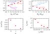 |
Fig. 5 Scatter diagrams of the correlated parameters. Panel a): κ (in 0.2 cm2/ g), Mej (in 7 M⊙), and ETh (in 3 foe) vs. R0; panel b): ESN (in 6 foe) and κ (in 0.2 cm2/ g) vs. Mej; panel c): κ vs. α; Panel d): Ep vs. tp. |
3. Comparison with observations and hydrodynamic models
In this section, we compare the parameters calculated from our radioactive energy input models with those from hydrodynamic simulations. We fit SNe 2004et, 2005cs, 2009N, 2012A, and 2012aw using our code using the radioactive energy input. Since our simple code is unable to capture the first post-breakout peak, the comparison between the data and the model was restricted to the later phases of the plateau and the radioactive tail.
Like most other SN modeling codes, our code needs the bolometric light curve, which is not observed directly. In order to assemble the bolometric light curves for our sample we applied the following steps. First, the measured magnitudes in all available photometric bands were converted into fluxes using proper zero points (Bessell et al. 1998), extinctions, and distances. The values of extinction in each case were taken from the NASA/IPAC Extragalactic Database (NED). At epochs when an observation with a certain filter was not available, we linearly interpolated the flux using nearby data. For the integration over wavelength, we applied the trapezoidal rule in each band with the assumption that the flux reaches zero at 2000 Ȧ. The infrared contribution was taken into account by the exact integration of the Rayleigh-Jeans tail from the wavelength of the last available photometric band (I or K) to infinity.
Note that to obtain a proper comparison with the other models collected from literature, we calculated the bolometric light curve using the same distance as in the reference papers.
3.1. SN 2004et
SN 2004et was discovered on 2004 September 27 by S. Moretti (Zwitter & Munari 2004). It exploded in a nearby starburst galaxy NGC 6946 at a distance of about 5.9 Mpc. This was a very luminous and well-observed Type IIP supernova (Sahu et al. 2006) in optical (UBVRI) and NIR (JHK) wavelengths. In this paper, all of these photometric bands were used to derive the bolometric light curve.
In the literature, SN 2004et was modeled with different approaches. Utrobin & Chugai (2009) used a 1-dimensional hydrocode to estimate the progenitor mass and other physical properties. Maguire et al. (2010) applied the formulae by Litvinova & Nadyozhin (1985) that are based on their hydrodynamical models, and also used the steepness parameter method from Elmhamdi et al. (2003), to get the physical parameters of SN 2004et. Table 2 shows the parameters from Maguire et al. (2010) and Utrobin & Chugai (2009) as well as our best-fit results. The bolometric light curve of SN 2004et and the model curve fitted using our code are plotted in Fig. 6.
Results for SN 2004et.
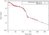 |
Fig. 6 Light curve of SN 2004et (dots) and the best result of our model (solid line). |
3.2. SN 2005cs
The underluminous supernova SN 2005cs was discovered on 2005 June 30 in M51 by Kloehr (2005). This event was more than a magnitude fainter than an average Type IIP supernova. Nevertheless, the light curve of SN 2005cs was observed in UBVRI bands and its physical properties were calculated by Tsvetkov et al. (2006) based on the hydrodynamic model of Litvinova & Nadyozhin (1985). SN 2005cs was also fitted using our code and the results can be found in Table 3. For better comparison, we used d = 8.4 Mpc for the distance of M51, which was adopted by Tsvetkov et al. (2006). However, we also calculated the quasi-bolometric light curve with d = 7.1 Mpc (Takáts & Vinkó 2006). The results for both distances are listed in Table 3. The best fit of our model can be seen in Fig. 7.
Results for SN 2005cs.
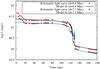 |
Fig. 7 Best fit for SN 2005cs (black line) and the bolometric luminosity at 8.4 Mpc (red dots). The orange circles represent the light curve of SN 2005cs at 7.1 Mpc and the gray line is our fit. |
3.3. SN 2009N
SN 2009N was discovered in NGC 4487 having a distance of 21.6 Mpc (Takáts et al. 2014). The first images were taken by Itagaki on 2009 Jan. 24.86 and 25.62 UT (Nakano et al. 2009). This event was not as luminous as a normal Type IIP SN, but it was brighter than the underluminous SN 2005cs. Hydrodynamic modeling was presented by Takáts et al. (2014) who applied the code of Pumo et al. (2010) and Pumo & Zampieri (2011). In Table 4, we summarize our results as well as the properties from hydrodynamic simulations. Figure 8 shows the luminosity from the observed data and the model light curve.
Results for SN 2009N.
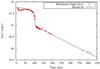 |
Fig. 8 Solid line shows the fit of our model and the dots represent bolometric luminosity from observed data of SN 2009N. |
3.4. SN 2012A
SN 2012A was discovered in an irregular galaxy NGC 3239 at a distance of 9.8 Mpc (Tomasella et al. 2013). The first image was taken on 2012 Jan. 7.39 UT by Moore, Newton & Puckett (2012). This event was classified as a normal Type IIP supernova with a short plateau. The luminosity drop after the plateau was intermediate between those of normal and underluminous Type IIP SNe. The fact that SN 2012A exploded in a nearby galaxy made this object very well-observed in multiple (UBVRIJHK) bands. For computing the physical properties of the progenitor, Tomasella et al. (2013) applied a semianalytical (Zampieri et al. 2003) and a radiation-hydrodynamic code (Pumo et al. 2010; Pumo & Zampieri 2011). Table 5 contains the final results of Tomasella et al. (2013) and our fitting parameters as well. Our model light curve can be seen in Fig. 9.
Results for SN 2012A.
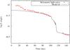 |
Fig. 9 Light curve of SN 2012A (dots) and the best result of our model (solid line). |
3.5. SN 2012aw
SN 2012aw was discovered on 2012 March 16.86 UT by P. Fagotti (Fagotti et al. 2012) in a spiral galaxy M95 at an average distance of 10.21 Mpc. This was a very well-observed Type IIP supernova in optical (UBVRI) and NIR (JHK) wavelengths (Dall’Ora et al. 2014). All of these photometric bands were used to create the bolometric light curve.
The physical properties of SN 2012aw modeled by Dall’Ora et al. (2014) who applied two different codes: a semianalytic (Zampieri et al. 2003) and a radiation-hydrodynamic code (Pumo et al. 2010; Pumo & Zampieri 2011). In Table 6 we summarize our result as well as the parameter values of Dall’Ora et al. (2014). Our best-fit model is plotted in Fig. 10.
Results for SN 2012aw.
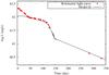 |
Fig. 10 Light curve of SN 2012aw (dots) and the best result of our model (solid line). |
4. Discussion and conclusion
The good agreement between the results from the analytical light curve modeling and the parameters from other hydrodynamic calculations leads to the conclusion that the usage of the simple analytical code may be useful for preliminary studies prior to more expensive hydrodynamic computation. The code described in this paper is also capable of providing quick estimates for the most important parameters of SNe such as the explosion energy, the ejected mass, the nickel mass, and the initial radius of the progenitor from the shape and peak of the light curve as well as its late-phase behavior. Note that there is a growing number of observational evidence showing that the plateau durations have a narrow distribution with a center at about 100 days (Faran et al. 2014), which suggests that strong correlations exist between parameters like the explosion energy and the progenitor radius in the presupernova stage. The code may offer a fast and efficient way to explore such type of parameter correlations.
Tables 2–6 show that the hydrodynamic models for Type IIP events consistently give higher ejected masses than our code. On the other hand, there are also major differences between the values given by different hydrocodes, such as in the case of SN 2004et. Although the total SN energies from our code are usually higher then those obtained from more complex models, they show a similar trend: for an underluminous SN the best-fit energy is lower, while for a more luminous SN the code suggests higher explosion energy.
The present code has various limitations and caveats. One of them is that it is not able to fit the light curve at very early epochs. This may be explained by the failure of the assumption of homologous expansion at such early phases, and/or the adopted simple form of the density profile. Another possibility could be the assumption of a two-component ejecta configuration, which is sometimes used for modeling Type IIb SNe (Bersten et al. 2012). In this case, the model also contains a low-mass envelope on top of the inner, more massive core. Within this context the fast initial decline may be due to radiation diffusion from the fast-cooling outer envelope heated by the shock wave due to the SN explosion. These models will be studied in detail in a forthcoming paper.
Acknowledgments
This work has been supported by Hungarian OTKA Grant NN 107637 (PI Vinko) and NSF Grant AST 11-09801 (PI Wheeler). We express our sincere thanks to an anonymous referee for the very thorough report that helped us a lot while correcting and improving the previous version of this paper.
References
- Arnett, W. D. 1980, ApJ, 237, 541 [Google Scholar]
- Arnett, W. D. 1982, ApJ, 253, 785 [NASA ADS] [CrossRef] [Google Scholar]
- Arnett, W. D., & Fu, A. 1989, ApJ, 340, 396 [NASA ADS] [CrossRef] [Google Scholar]
- Bessell, M. S., Castelli, F., & Plez, B. 1998, A&A, 333, 231 [NASA ADS] [Google Scholar]
- Blinnikov, S., Lundqvist, P., Bartunov, O., et al. 2000, ApJ, 532, 1132 [NASA ADS] [CrossRef] [Google Scholar]
- Bersten, M. C., Benvenuto, O., & Hamuy, M. 2011, ApJ, 729, 61 [NASA ADS] [CrossRef] [Google Scholar]
- Bersten, M. C., Benvenuto, O. G., Nomoto, K., et al. 2012, ApJ, 757, 31 [NASA ADS] [CrossRef] [Google Scholar]
- Chatzopoulos, E., Wheeler, J. C., & Vinkó, J. 2012, ApJ, 746, 121 [NASA ADS] [CrossRef] [Google Scholar]
- Dall’Ora, M., Botticella, M. T., Pumo, M. L., et al. 2014, ApJ, 787, 139 [NASA ADS] [CrossRef] [Google Scholar]
- Elmhamdi, A., Chugai, N. N., & Danziger, I. J. 2003, A&A, 404, 1077 [NASA ADS] [CrossRef] [EDP Sciences] [Google Scholar]
- Fagotti, P., Dimai, A., Quadri, U., et al. 2012, CBET, 3054, 1 [Google Scholar]
- Falk, S. W., & Arnett, W. D. 1977, ApJS, 33, 515 [NASA ADS] [CrossRef] [Google Scholar]
- Faran, T., Poznanski, D., Filippenko, A. V., et al. 2014, MNRAS, 442, 844 [NASA ADS] [CrossRef] [Google Scholar]
- Grassberg, E. K., & Nadyozhin, D. K. 1976, Ap&SS, 44, 409 [NASA ADS] [CrossRef] [Google Scholar]
- Grassberg, E. K., Imshennik, V. S., & Nadyozhin, D. K. 1971, Ap&SS, 10, 28 [NASA ADS] [CrossRef] [Google Scholar]
- Hatano, K., Branch, D., Fisher, A., et al. 1999, ApJS, 121, 233 [NASA ADS] [CrossRef] [Google Scholar]
- Hillebrandt, W., & Müller, E. 1981, A&A, 103, 147 [NASA ADS] [Google Scholar]
- Kasen, D., & Bildsten, L. 2010, ApJ, 717, 245 [NASA ADS] [CrossRef] [Google Scholar]
- Kloehr, W. 2005, IAU Circ., 8553, 1 [NASA ADS] [Google Scholar]
- Litvinova, I. Y., & Nadyozhin, D. K. 1985, Sov. Astron. Lett., 11, 145 [NASA ADS] [Google Scholar]
- Maguire, K., Di Carlo, E., Smartt, S. J., et al. 2010, MNRAS, 404, 981 [NASA ADS] [CrossRef] [Google Scholar]
- Moore, B., Newton, J., & Puckett, T. 2012, CBET, 2974, 1 [NASA ADS] [Google Scholar]
- Nadyozhin, D. K. 2003, MNRAS, 346, 97 [NASA ADS] [CrossRef] [Google Scholar]
- Nakano, S., Kadota, K., & Buzzi, L. 2009, CBET, 1670, 1 [NASA ADS] [Google Scholar]
- Piro, A. L., & Ott, C. D. 2011, ApJ, 736, 108 [NASA ADS] [CrossRef] [Google Scholar]
- Popov, D. V. 1993, ApJ, 414, 712 [Google Scholar]
- Pumo, M. L., & Zampieri, L. 2011, ApJ, 741, 41 [NASA ADS] [CrossRef] [Google Scholar]
- Pumo, M. L., Zampieri, L., & Turatto, M. 2010, MSAIS, 14, 123 [NASA ADS] [Google Scholar]
- Sahu, D. K., Anupama, G. C., Srividya, S., et al. 2006, MNRAS, 372, 1315 [NASA ADS] [CrossRef] [Google Scholar]
- Takáts, K., & Vinkó, J. 2006, MNRAS, 372, 1735 [NASA ADS] [CrossRef] [Google Scholar]
- Takáts, K., Pumo, M. L., Elias-Rosa, N., et al. 2014, MNRAS, 438, 368 [NASA ADS] [CrossRef] [Google Scholar]
- Tomasella, L., Cappellaro, E., Fraser, M., et al. 2013, MNRAS, 434, 1636 [NASA ADS] [CrossRef] [Google Scholar]
- Tsvetkov, D. Y., Volnova, A. A., Shulga, A. P., et al. 2006, A&A, 460, 769 [NASA ADS] [CrossRef] [EDP Sciences] [Google Scholar]
- Utrobin, V. D. 2007, A&A, 461, 283 [Google Scholar]
- Utrobin, V. D., & Chugai, N. N. 2009, A&A, 506, 829 [NASA ADS] [CrossRef] [EDP Sciences] [Google Scholar]
- Utrobin, V. D., Chugai, N. N., & Pastorello, A. 2007, A&A, 475, 937 [Google Scholar]
- Woosley, S. E. 2010, ApJ, 719, L204 [NASA ADS] [CrossRef] [Google Scholar]
- Zampieri, L., Pastorello, A., Turatto, M., et al. 2003, MNRAS, 338, 711 [NASA ADS] [CrossRef] [Google Scholar]
- Zwitter, T., & Munari, U. 2004, IAU Circ., 8413, 1 [NASA ADS] [Google Scholar]
All Tables
All Figures
|
Fig. 1 Model light curve computed with exact sin(πx)/(πx) temperature profile (black) and with 4th order Taylor series (red). |
| In the text | |
|
Fig. 2 Effect of changing the initial radius of the ejecta (panel a)), the ejected mass (panel b)), the initial nickel mass (panel c)), and the recombination temperature (panel d)). |
| In the text | |
|
Fig. 3 Effect of changing the initial kinetic energy (panel a)), the initial thermal energy (panel b)), the density profile exponent (panel c)), and the opacity (panel d)). |
| In the text | |
|
Fig. 4 Effect of changing the initial rotation energy of the magnetar (panel a)), the characteristic timescale of magnetar spin-down (panel b)), the gamma-ray leakage exponent (panel c)). |
| In the text | |
|
Fig. 5 Scatter diagrams of the correlated parameters. Panel a): κ (in 0.2 cm2/ g), Mej (in 7 M⊙), and ETh (in 3 foe) vs. R0; panel b): ESN (in 6 foe) and κ (in 0.2 cm2/ g) vs. Mej; panel c): κ vs. α; Panel d): Ep vs. tp. |
| In the text | |
|
Fig. 6 Light curve of SN 2004et (dots) and the best result of our model (solid line). |
| In the text | |
|
Fig. 7 Best fit for SN 2005cs (black line) and the bolometric luminosity at 8.4 Mpc (red dots). The orange circles represent the light curve of SN 2005cs at 7.1 Mpc and the gray line is our fit. |
| In the text | |
|
Fig. 8 Solid line shows the fit of our model and the dots represent bolometric luminosity from observed data of SN 2009N. |
| In the text | |
|
Fig. 9 Light curve of SN 2012A (dots) and the best result of our model (solid line). |
| In the text | |
|
Fig. 10 Light curve of SN 2012aw (dots) and the best result of our model (solid line). |
| In the text | |
Current usage metrics show cumulative count of Article Views (full-text article views including HTML views, PDF and ePub downloads, according to the available data) and Abstracts Views on Vision4Press platform.
Data correspond to usage on the plateform after 2015. The current usage metrics is available 48-96 hours after online publication and is updated daily on week days.
Initial download of the metrics may take a while.