| Issue |
A&A
Volume 570, October 2014
|
|
|---|---|---|
| Article Number | A72 | |
| Number of page(s) | 9 | |
| Section | Extragalactic astronomy | |
| DOI | https://doi.org/10.1051/0004-6361/201424622 | |
| Published online | 21 October 2014 | |
The dichotomy of Seyfert 2 galaxies: intrinsic differences and evolution
Institute for Astronomy and Astrophysics, Space Applications and Remote
Sensing, National Observatory of Athens,
15236
Palaia Penteli Athens,
Greece
e-mail:
This email address is being protected from spambots. You need JavaScript enabled to view it.
Received:
17
July
2014
Accepted:
20
August
2014
Abstract
We present a study of the local environment (≤200 h-1 kpc) of 31 hidden broad line region (HBLR) and 43 non-HBLR Seyfert 2 (Sy2) galaxies in the nearby universe (z ≤ 0.04). To compare our findings, we constructed two control samples that match the redshift and the morphological type distribution of the HBLR and non-HBLR samples. We used the NASA Extragalactic Database (NED) to find all neighboring galaxies within a projected radius of 200 h-1 kpc around each galaxy, and a radial velocity difference δu ≤ 500 km s-1. Using the digitized Schmidt survey plates (DSS) and/or the Sloan Digital Sky Survey (SDSS), when available, we confirmed that our sample of Seyfert companions is complete. We find that, within a projected radius of at least 150 h-1 kpc around each Seyfert, the fraction of non-HBLR Sy2 galaxies with a close companion is significantly higher than that of their control sample, at the 96% confidence level. Interestingly, the difference is due to the high frequency of mergers in the non-HBLR sample, seven versus only one in the control sample, while they also present a high number of hosts with signs of peculiar morphology. In sharp contrast, the HBLR sample is consistent with its control sample. Furthermore, the number of the HBLR host galaxies that present peculiar morphology, which probably implies some level of interactions or merging in the past, is the lowest in all four galaxy samples. Given that the HBLR Sy2 galaxies are essentially Seyfert 1 (Sy1) with their broad line region (BLR) hidden because of the obscuring torus, while the non-HBLR Sy2 galaxies probably also include true Sy2s that lack the BLR as well as heavily obscured objects that prevent even the indirect detection of the BLR, our results are discussed within the context of an evolutionary sequence of activity triggered by close galaxy interactions and merging. We argue that the non-HBLR Sy2 galaxies may represent different stages of this sequence, possibly the beginning and the end of the nuclear activity.
Key words: galaxies: active / galaxies: nuclei / galaxies: Seyfert / galaxies: evolution / galaxies: interactions
© ESO, 2014
1. Introduction
Polarized emission from the central engine of active galactic nuclei (AGN) can be produced by the reflection of radiation from a scattering media. Evaporated gas that originated in the inner surface of the obscuring matter near the central black hole can escape the area and form such a mirror in a favorable location where the light can be reflected toward the observer without being absorbed. Thus, polarized light is a powerful tracer of AGN activity, otherwise hidden due to obscuration along our line of sight (e.g., Krolik 1999).
Nearly thirty years ago, the first discovery by Miller & Antonucci (1983) of broad permitted emission lines and a clearly non-stellar continuum in the polarized spectrum of the archetypal Seyfert 2 (Sy2), NGC 1068, was just the beginning of numerous similar observations in a wide variety of galaxies. Ten years later, the unification model (UM) of AGN was formulated upon these observations (Antonucci 1993). According to the UM, all Seyfert nuclei are intrinsically identical, while the only cause of their different observational features is the orientation of an obscuring torus with respect to our line of sight. A hidden broad line region (HBLR) was considered to be present in all Type II active galaxies, visible to us only by the reflection of a fraction of the total emitted radiation.
Nevertheless, polarization has also been a basis on which the unified scheme was questioned, since Tran (2001, 2003) concluded that there is a non-HBLR Sy2 population significantly different from the corresponding HBLR Sy2 population. He argued that, in contrast to the HBLR Sy2s, the true Sy2 AGN are intrinsically less powerful and they cannot be fitted within the realm of the UM. The same conclusion was reached in recent statistical studies (e.g., Tommasin et al. 2010; Wu et al. 2011). Many authors argue that the lack of a broad line region (BLR) in the center of these Sy2 galaxies is luminosity and/or accretion rate dependent (Nicastro 2000; Lumsden & Alexander 2001; Gu & Huang 2002; Martocchia 2002; Panessa & Bassani 2002; Tran 2003; Nicastro et al. 2003; Laor 2003; Czerny et al. 2004; Elitzur & Shlosman 2006; Elitzur 2008; Elitzur & Ho 2009; Marinucci 2012; Elitzur et al. 2014). Low luminosity can be the result of very low accretion rate and the BLR may possibly be absent in such systems.
In addition, although widely accepted today, the UM cannot explain various observed differences between Type I and Type II AGN. Many studies over the years challenged its validity and proposed instead an evolutionary sequence that links different types of activity (e.g., Hunt & Malkan 1999; Dultzin-Hacyan 1999; Krongold et al. 2002; Levenson et al. 2001; Koulouridis et al. 2006a,b, 2013). In particular, although the role of interactions on induced activity is still an open issue (Koulouridis et al. 2006a,b, 2013, and references therein), most of the above studies seem to conclude that the possible evolution of activity follows the path of interactions → enhanced star formation → Type II AGN → Type I AGN. However, their Sy2 samples were never examined for the possible existence of hidden broad lines since spectropolarimetric observations are time-consuming and are feasible only with large telescopes.
Koulouridis et al. (2006a) compared the environment of two samples of Seyfert 1 (Sy1) and Sy2 galaxies to that of two well-defined control samples, concluding that the Sy2 sample shows an excess of close companions, while the Sy1 sample did not. In addition, Koulouridis et al. (2013) showed that the neighbors of Sy2 galaxies are systematically more ionized than the neighbors of Sy1 galaxies, a fact that indicates differences in metallicity, stellar mass, and star-formation history between the samples. In the current study we focus solely on Sy2 galaxies by investigating the environment of the biggest compiled HBLR and non-HBLR samples to date, in order to discover possible differences between the two that can provide us with additional clues about the nature of these objects.
We describe our samples and methodology in Sect. 2, our results in Sect. 3, and our conclusions and discussion in Sect. 4. Throughout this paper we use H0 = 73 km s-1/Mpc, Ωm = 0.27, and ΩΛ = 0.73.
2. Sample selection and methodology
2.1. On the non-HBLR population
Although the existence of non-HBLR Sy2s can be succesfully explained by the true Sy2 interpretation, this is not the only solution to the lack of observed broad emission lines (see also Antonucci 2012). As indicated by previous studies (e.g., Wu et al. 2011), in spite of the overal differences, the properties of a fraction of the non-HBLR Sy2s are very similar to the properties of the HBLR Sy2s. Therefore, we argue that we can divide the non-HBLR Sy2s into three main categories based on their obscuration:
-
1.
true Sy2s, that do not present broad emission lines in their spectra, but at the same time are not obscured (e.g., Panessa & Bassani 2002; Akylas & Georgantopoulos 2009);
-
2.
heavily obscured, so that the presence of a possible BLR cannot be detected in any way;
-
3.
mildly obsured, so that the BLR was possibly not observed because of other limitations, e.g., observational flux limit, host galaxy obscuration, bad orientation, or total lack of the scattering matterial that produces the polarized broad lines (if this is not the same as the obscuring matterial).
Only in the first case can we be almost certain that the object does indeed lack the BLR and it is intrisically different from a broad line Seyfert. In the other two cases the BLR can either be present or not. Therefore, we should clearly state once more that the current study investigates two samples of HBLR and non-HBLR Sy2s, without making any other assumption on the nature of these objects. The discovery of any differences in the environment of these two samples may indicate intrinsic differences between the two populations that do not necessarily apply to all objects individualy.
2.2. Sample selection
The original HBLR and non-HBLR Sy2 galaxy samples can be found in Wu et al. (2011). From this sample we excluded all galaxies with z ≥ 0.04 since above this limit their morphological type is usually undefined and the number of probable neighbors with no redshift becomes very large for our statistics. In addition, we find that even their classification as Sy2 is uncertain, let alone the detection of polarized broad emission lines. The detection is dubious because in order to calculate the polarized fraction of the reflected light, the stellar contribution must be subtracted, which is more difficult for smaller objects where more starlight is included in the observed spectrum (Krolik 1999). From the original catalogue we also excluded the 18 Sy2s that have no spectropolarimetric observations but were classified using other criteria by Wang & Zhang (2007). Finally, a small number of faint galaxies were excluded independently of their redshift.
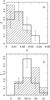 |
Fig. 1 Redshift (panel a)) and Morphological type (panel b)) distribution of the Sy2 samples. The solid line defines the HBLR Sy2 population, while the hatched histogram the non-HBLR. Uncertainties are 1σ Poissonian errors and they are plotted only for the HBLR Sy2s for clarity. |
The redshift and the morphological type distribution of the two Seyfert samples are presented in Fig. 1. The distributions do differ, especially the morphological, although their differences are not statistically significant. An interesting trend is that the HBLR Sy2s are hosted by earlier-type galaxies than the non-HBLR. This trend is already known for the Sy1 and Sy2 hosts, where the former show the same behavior as the HBLR Sy2 hosts. This supports the interpretation that the HBLR Sy2s are indeed Sy1s with their broad line region obscured by a dusty torus, but reflected by a scattering surface located over the torus. On the other hand, this trend already implies intrinsic differences between the two Sy2 types. Because of these differences in the distributions, we do not proceed with a direct comparison of the environment of our two samples. The slightly different redshift distribution may introduce a bias against the detection of HBLR Sy2 neighbors because the higher the redshift, the higher the probability of fainter neighbors with unknown redshift. On the other hand, the different morphological type distributions may lead to the opposite direction, since it is well known that early-type galaxies are more clustered than late-types. Thus, we choose to build two control samples that have the same redshift and morphological type distribution with the two Sy2 samples, respectively. Any comparison will be made between each Sy2 and its control sample and the conclusions will be drawn from there.
The control samples were randomly built from the NGC, MRK, and IC databases. All objects that had any reference of being active (AGN or LINER) were excluded and replaced, and finally the samples were refined so as to match the redshift and morphological type distribution of the HBLR and non-HBLR samples. To have a homogeneous morphological classification we chose to use the types listed in the Third Reference Catalogue of bright galaxies (RC3). We should note that peculiarity was not taken into consideration when constructing the control samples as this could bias our results, i.e., a peculiar Sa galaxy is treated like an Sa for our purposes. In addition, galaxies classified solely as peculiars were not included in the morphological type distribution matching at all. In more detail, in the control samples we did not attempt to include the same number of peculiar galaxies that we found in the Seyfert samples. The reason is that peculiar galaxies may have undergone a recent merger or may be still strongly interacting with a close companion. Forcing the same number of peculiar galaxies in the control sample could artificially enhance the number of interacting galaxies.
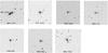 |
Fig. 2 Images of the merging galaxies in our samples. |
2.3. Methodology
In order to identify possible neighbors around each Sy2 and control sample galaxy, we made use of the automated search of the NASA/IPAC Extragalactic Database. In the current study we do not discriminate between galaxy pair and satellite galaxies. All galaxies that meet the qualifying criteria described below are considered as neighbors of the investigated galaxy:
-
galaxies within a projected radius of 200 h-1 kpc from the AGN or the control galaxy,
-
galaxies with a radial velocity difference of δu ≤ 500 km s-1.
Even though there is no general consensus on the maximum radial separation of a galaxy pair, most of the recent studies use a search radius between 20 h-1 kpc (e.g., Patton et al. 2005) and 200 h-1 kpc (e.g., Focardi et al. 2006; see also relevant discussion in Deng et al. 2008). We chose the limit of 200 h-1 kpc considering that it is a reasonable distance for a satellite galaxy in a massive halo (e.g., Bahcall et al. 1995; Zaritsky et al. 1997). Distances were estimated taking into account the local velocity field, which includes the effects of Virgo, Great Attractor and Shapley, for the standard ΛCDM cosmology (Ωm = 0.27, ΩΛ = 0.73) Since, however, NED is not complete in any way, we also visually inspected all DSS or SDSS images (when available) to discover any other neighbor candidates with no listed redshift. Only four possible neighbours with no available spectroscopic redshift were found, two of the HBLR and two of their control sample. However, based on SDSS photometric redshifts that were available for all four objects, we chose to exclude them from the analysis since they were incompatible with the sample galaxy redshift, even within the errors. We note that the inclusion of these four objects would not alter the results. Finally, we classified the companion galaxies based on their magnitude difference (Δm) with the sample galaxy by using a common blue magnitude, mostly from the RC3 or the SDSS database, i.e., the neighbors with 2 < Δm ≤ 3 were classified as small and were treated separately, while those with Δm> 3 were not included in this analysis. In addition, above 100 h-1 kpc small neighbors were not included. Mergers were regarded as galaxies in strong interaction regardless of the magnitude difference of the pre-merging galaxies, which is unknown in many cases. A wide range of cases were considered as mergers, from the case of two clearly separated but nevertheless very close galaxies with clear signs of strong interactions (e.g., NGC 1143 and NGC 1144) to the case of post-mergers with peculiar morphology, only if reported as such in the literature (e.g., MRK 334). The images of all the merger galaxies can be found in Fig. 2. Finally, we note that MRK 1039 and MRK 1066 are reported as galaxies with double nucleus. We chose to include them as mergers (probably in an advanced stage).
HBLR Sy2 and control sample.
Non-HBLR Sy2 and control sample.
Our final Seyfert samples consist of 43 non-HBLR, 31 HBLR Sy2s, and their control samples (a total of 148 galaxies). The galaxy redshift, the morphological type and the projected distance to their neighbors are given in Tables 1 and 2. Our search radius of 200 h-1 kpc was divided into four bins of 50 h-1 kpc and each neighbor was placed accordingly. In the current study we are mostly interested in addressing the following two questions:
-
a.
Is there any significant difference between the fraction ofSeyferts and the fraction of their respective control samplegalaxies that have at least one neighbor within a given radius?
-
b.
Is there any significant difference between the density of the environment where the Seyferts and their respective control sample are found?
A positive answer to either question will imply that there are intrinsic differences between the investigated samples, and that the environment probably plays a leading role in the creation of these differences. The answer to the first question will show us if interaction with a close neighbor can play the role of the triggering mechanism that leads to the detected differences, while to the second will provide us with information about the general local environment. We should stress that in the present study we are not interested in the large-scale environment of our sample galaxies. This will probably not differ between each Seyfert sample and its respective control sample, since they were selected to have the same redshift and, especially, morphological type distribution. However, the local environment may vary, as shown in Koulouridis et al. (2006a,b), independently of the density of the large-scale environment. Even the presence of a single neighbor of comparable mass, within a certain radius, may introduce the necessary conditions that would lead to the detected differences.
3. Results
In Tables 1 and 2 we listed all our galaxies, active and control, and their close companions divided into four bins depending on their radial separation. With the symbol “x” we mark all neighbors that are no more than two magnitudes fainter than the galaxy in question, while with “s” the ones that are between two and three magnitudes fainter. The selection of these specific limits is not random, but was decided after visual inspection of the neighbors. Some characteristic examples can be found in Fig. 3, where we can see that in contrast to neighbors with δm< 2, the ones above this limit are becoming rather small in comparison and their capability of producing any sufficient interactions can be questioned. In addition, in the case of higher redshift galaxies and those in regions with significant star contamination, faint neighbors may be missed, although these effects will probably affect equally the Seyfert samples and their control. For these reasons, although listed in the tables, small galaxies were not considered when we extracted our main results, and their possible role is only discussed briefly. Given their ambiguous role even in small radial distances, above 100 h-1 kpc small neighbors are not listed at all. Finally, for a small number of cases, the decision whether the companion is large or small had to be made after visual investigation because of lack of data. These cases are marked with a star.
To draw our conclusions we will refer to the results of a number of statistical tests. First, we ran the Fisher’s exact test for a 2 × 2 contingency table to compare the fraction of Seyferts and the fraction of their respective control sample galaxies that have at least one neighbor within a given radius (question a. in the methodology). Each row of the contingency table is one of the two samples (Seyfert and respective control sample), while the input in the two columns is the number of galaxies that have a companion (Col. 1) and do not have one (Col. 2) within a certain radius. Therefore, the sum of the two columns of each row gives us the total number of galaxies in each sample. The results of the tests are listed in the last row of Tables 1 and 2. We list the results of four tests in each table, depending on the radial distance we chose to search for neighbors. We always consider previous radial bins in the total, i.e., the second value in Table 1 (Pnull = 0.7723) refers to the comparison of the total number of HBLR Sy2 and control sample galaxies that have companions within 100 h-1 kpc (not between 50 and 100 h-1 kpc); Pnull is the probability that the two samples are drawn from the same parent population. For the HBLR Sy2 and its control sample, independent of the search radius, the results suggest that the null hypothesis cannot be rejected at any significant statistical level, and thus the two samples are probably drawn from the same parent population. In sharp contrast, the non-HBLR and its control sample do indeed differ at a high statistical level in the first three bins (>96%), and at a moderate level in the fourth. We note that for the non-HBLR analysis, the one-sided test was used, since we already suspected from our previous works (Koulouridis et al. 2006a,b, 2013) that a real Seyfert 2 population will present more companions than their control sample galaxies. We note, however, that the two-sided test results are two times the one-sided results, and therefore by using it we would reach qualitatively the same conclusions, although after the inclusion of the last bin there would be no statistically significant difference at any level between the two samples.
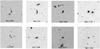 |
Fig. 3 Examples of Seyferts and control sample galaxies with companions. Small companions are marked with the letter s. In the case of NGC 7582, another non-HBLR Sy2, NGC 7590 is one of the close neighbors. |
Independently of the results of the previous paragraph, to compare the density of the environment that the Seyferts and their respective control sample are embedded in (question b. in the methodology), we calculated the mean number of galaxies that are found within a 200 h-1 kpc radius around all the galaxies of each sample. Then, we tested how statistically significant the difference of the means is, by calculating the error σ of these differences with the formula
![Mathematical equation: $$ \sigma=\sqrt{\frac{(n_1-1)S_1^2+(n_2-1)S_2^2}{n_1+n_2-2}\left[\frac{1}{n_1}+\frac{1}{n_2}\right]}, $$](/articles/aa/full_html/2014/10/aa24622-14/aa24622-14-eq28.png) where n1 and
n2
are the number of sample galaxies and S1 and S2 the standard
deviation. In the case of the HBLR Sy2s and their control sample σ = 0.228, and the difference
of the means is
where n1 and
n2
are the number of sample galaxies and S1 and S2 the standard
deviation. In the case of the HBLR Sy2s and their control sample σ = 0.228, and the difference
of the means is  , where
 is the mean
number of companions in each sample. These results show that the environments of the two
populations are different at the 97.8% level, with the Sy2s showing a preference for less
dense environments. Similarly, for the non-HBLR and its control sample the respective values
are
is the mean
number of companions in each sample. These results show that the environments of the two
populations are different at the 97.8% level, with the Sy2s showing a preference for less
dense environments. Similarly, for the non-HBLR and its control sample the respective values
are  with σ = 0.218 and again the
difference of the means is statistically highly significant, at the 98.9% level. However, in
this case, the preference of the Sy2 population is for the denser environments.
with σ = 0.218 and again the
difference of the means is statistically highly significant, at the 98.9% level. However, in
this case, the preference of the Sy2 population is for the denser environments.
Finally, we attempted to compare more directly the two Sy2 populations by calculating the
overdensity of companions around each host. This overdensity measure is given by the
formula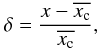 where
x is the
number of neighbors around each Sy2 host, and
where
x is the
number of neighbors around each Sy2 host, and  is the mean number of companions derived from the control sample. In this way we took into
consideration the information of the control sample, while at the same time we only had two
sets of numbers to compare, the overdensities of the HBLR and the non-HBLR Sy2s. We ran a
Kolmogorov-Smirnov test and we concluded that the overdensities differ at a very high
statistical level (>99.9%).
is the mean number of companions derived from the control sample. In this way we took into
consideration the information of the control sample, while at the same time we only had two
sets of numbers to compare, the overdensities of the HBLR and the non-HBLR Sy2s. We ran a
Kolmogorov-Smirnov test and we concluded that the overdensities differ at a very high
statistical level (>99.9%).
We note that small neighbors were not considered in the above statistical analyses for the reasons we described in the methodology. However, we mention that this could affect mostly the Fisher’s exact test for the non-HBLR and its control sample because there is a number of small galaxies to be found within the first 50 h-1 kpc around the control galaxies. None of the remaining results would change significantly. We also note that the control galaxy NGC 4488 is located within a galaxy cluster and, as noted in Table 1, a large number of companions can be found in its third and fourth bin. However, for the statistical analyses we chose to consider only two companions in each bin, because otherwise we believe that the results would be biased.
Interestingly, we note the relatively large number of mergers and peculiar host morphologies in the non-HBLR sample in comparison to their control sample. In particular, the merger fraction is significantly higher when compared to any of our samples. These facts corroborate with our findings that the non-HBLR host galaxies reside in denser environments when compared with their control sample and a significantly larger fraction of them presents at least one companion within 200 h-1 kpc. In many cases, by visual investigation of the DSS and/or the SDSS images, we can clearly identify the companion galaxy or merging as the reason for the peculiar morphology. However, this is only visible in the case of close pairs (D< 30 h-1 kpc), while for galaxies with no companion, the peculiar morphology probably suggests past interactions/merging or even false classification. On the other hand, the HBLR Sy2 sample has only three hosts with signs of peculiar morphology, less than half of its control sample, which again agrees with their preference for less dense environments and fewer interactions.
4. Discussion and conclusions
Investigating the environments of two samples of HBLR and non-HBLR Sy2s, we reached the conclusion that there is a statistically significant difference between the two types of Sy2 galaxies and their respective control samples. The non-HBLR population have neighbors more frequently than their control sample galaxies, within the specified spatial and velocity limits. Also, they are found more often in denser close environments than galaxies of the same morphological type, and the frequency of merging and peculiar morphologies is also relatively high. On the contrary, HBLR Sy2s are found in less dense environments than their control sample, and the frequency of merging or any sign of interactions is also low. In addition, their fraction with at least one neighbor agrees with the control galaxies, in all search radii. These results are also in agreement with our previous studies on Seyfert galaxies and they indicate the similarities between HBLR Sy2 and Sy1 galaxies, supporting the view that in all probability they are intrinsically the same objects. However, non-HBLR Sy2 galaxies seem to differ significantly, although their nature is still a matter of debate. Therefore, in the light of the current results, we will discuss probable mechanisms responsible for the observed and possibly intrinsic differences.
There is strong evidence that the dusty obscuring torus in low luminosity AGN is absent or is thinner than expected in higher luminosities (e.g., Whysong & Antonucci 2004; Elitzur & Shlosman 2006; Perlman et al. 2007; van der Wolk et al. 2010). Accordingly, all low luminosity AGN should have been Type I sources, which of course is not the case. The only reasonable explanation to this problem is the additional absence of the BLR in such systems. As we have noted earlier, some authors (e.g., Nicastro 2000; Nicastro et al. 2003; Bian et al. 2007; Marinucci et al. 2012; Elitzur et al. 2014) presented arguments that below a specific accretion rate of material into the black hole, and therefore at lower luminosities, the BLR might be absent. Elitzur & Ho (2009), using data from nearby bright AGN, concluded that the BLR disappears at bolometric luminosities lower than 5 × 1039(M/ 107M⊙)2 / 3 ergs-1, where M is the mass of the black hole. They also argued that the quenching of the BLR, and the disappearance of the torus can occur either simultaneously or in sequence, with decreasing black hole accretion rate and luminosity. Thus, a possible scenario would be that non-HBLR Sy2 AGN are objects lacking the BLR and possibly the torus. Bian et al. (2007) and Wu et al. (2011) separate their non-HBLR sample into luminous and less luminous using the log L[ OIII ]< 41 limit, while Marinucci et al. (2012), argued that true Sy2s can be found below the bolometric luminosity limit log Lbol = 43.9. We should note that in Marinucci et al. (2012) they derived the bolometric luminosity from the X-ray and the [OIV] luminosity and concluded that L[ OIII ] is not as reliable (see also relevant discussion in Elitzur 2012).
An alternative scenario is that heavy obscuration in non-HBLR Sy2 does not allow the detection of the BLR even in the polarized spectrum. Marinucci et al. (2012) concluded that 64% of their compton-thick non-HBLR Sy2s exhibit higher accretion rates than the threshold clearly separating the two Sy2 classes. They attributed this discrepancy to heavy absorption along our line of sight, preventing the detection of the actual BLR in their nuclei. Evidently, merging systems constitute a class of extragalactic objects where heavy obscuration occurs (e.g., Hopkins et al. 2008). The merging process may also lead to rapid black hole growth, giving birth to a heavily absorbed and possibly compton-thick AGN. Thus, we could presume that a fraction of our non-HBLR mergers, if not all of them, might actually be BLR AGN galaxies, where the large concentration of gas and dust prohibits even the indirect detection of the broad line emission (e.g., Shu et al. 2007). However, other studies concluded that there is no evidence that non-HBLR Sy2s are more obscured than their HBLR peers (Tran 2003; Yu 2005; Wu 2011), while totally unobscured low-luminosity non-HBLR Sy2s were detected via investigation of their X-ray properties (e.g., Panessa & Bassani 2002; Akylas & Georgantopoulos 2009). The total population of non-HBLR Sy2s is probably a mixture of objects with low accretion rate and/or high obscuration.
Both scenarios agree with the interpretation of our current results by the evolutionary scheme proposed by Krongold et al. (2002) and supported later by Koulouridis et al. (2006a,b, 2013), according to which, interaction with a comparable sized galaxy can drive molecular clouds toward the nucleus and trigger an evolutionary sequence, going from enhanced star formation to obscured Type II and finally to Type I activity. If the first scenario is valid, it is to be expected that during the initial stage of the interaction the accretion rate of the central black hole would be low and there would be neither a BLR nor a torus. In addition, as already discussed, heavy absorption caused by the interaction may also prevent the detection of the possibly existing BLR during the first stage of the AGN cycle. Consequently, the first stage of nuclear activity should be a non-HBLR narrow line AGN. Evidently, 71% of the non-HBLR Sy2 galaxies, with at least one neighbor within 100 h-1 kpc and/or peculiar morphology, have high obscuration (NH> 1024) and/or low luminosity (log L[ OIII ]< 41; criterion by Wu et al. 2011). For another 19% we do not have the information, while only 10% of them are reported as luminous and at the same time unabsorbed sources. Although these fractions may vary depending on the BLR-disappearance luminosity limit, we should mention than more than half of our objects have column densities that characterize Compton-thick AGNs. In addition, our non-HBLR sample contains only ten galaxies (23%) with log L[ OIII ]< 41, which can be considered as low luminosity, while all HBLR Sy2s are above that limit. However, this classification should not be considered explicit. We argue that the lack of the BLR is not due to low luminosity per se, but rather to their being at the start of the activity duty cycle, which renders them less powerful than the ones that already have formed a BLR. Therefore, the actual value of the luminosity is not so relevant for the comparison, but instead the fact that as a whole the non-HBLR population would be less luminous than the respective HBLR. Indeed, a Kolmogorov-Smirnov test indicates that the luminosity distributions of our two Seyfert samples are significantly different at the 98.7% level, with the HBLR Sy2s being shifted toward higher luminosities. In addition, Ho et al. (2012) and Miniutti et al. (2013) report AGNs with very high Eddington ratios, but very low black hole masses and no broad lines (see also Wang et al. 2012). Because of their high Eddington ratios, both objects greatly exceed the luminosity limits above which, previous studies argue, the BLR should be present, and provide observational evidence that true Sy2s can have higher luminosities.
The accretion rate and luminosity increase can generate the BLR and also anticipate the heavy obscuration, leading to the HBLR-Sy2 and finally Sy1 phase. However, the time needed for Type I activity to appear should be larger than the timescale for an unbound companion to escape from the close environment, or comparable to the timescale needed for an evolved merger (~1 Gyr, see Krongold et al. 2002). This delay is a possible explanation for the lack of close neighbors around the HBLR Sy2 and Sy1 galaxies (see Koulouridis et al. 2006a, 2013) and for the earlier-type morphologies of their hosts. If the evolutionary scenario is valid, unobscured Type I AGN can only exist after the dissipation of the obscuring media and the strangulation of the star forming activity by the AGN feedback (Krongold et al. 2007, 2009; Hopkins & Elvis 2010; see also the disk wind scenario in Elitzur & Shlosman 2006).
On the other hand, about half of the non-HBLR Sy2s seem isolated and undisturbed. These objects do not seem to be either just triggered or heavily obscured by recent close interactions. However, if the low accretion rate scenario is valid, one would expect that AGN should also lose their BLR at the end of the AGN duty cycle, as the accretion rate drops below a critical value (e.g., Bian et al. 2007; Elitzur & Ho 2009; Elitzur et al. 2014). Denney et al. (2014) argue that NGC 590 is an example of a Seyfert 1 that changed to Type 1.9 in less than 40 years, and that this is due to a significant luminosity, and therefore accretion rate, decrease. However, the morphological type distribution of the non-HBLR Sy2 host galaxies (as we saw earlier in Fig. 1) peaks at even later-type spirals than the corresponding distribution of the HBLR sample, although the difference is not statistically significant. This implies that the majority of these galaxies are still unevolved. Even though the morphology of such a galaxy could oscillate from late to early types up to four times, depending strongly on the environment and cold gas availability (Bournaud & Combes 2002), the older stellar population of the HBLR Sy2 and Sy1 hosts, compared to the non-HBLR, reported by Wu et al. (2011), provides some evidence that non-HBLR Sy2 galaxies probably precede the broad line phase (however, see Yu et al. 2013). However, although we cannot conclude positively about this scenario, it agrees perfectly well with the final stage of the evolutionary scenario.
Considering all the above, HBLR and non-HBLR Sy2s can be fitted within the AGN evolutionary scheme as described qualitatively in Fig. 4 (see also Fig. 17 of Wang & Zhang 2007 for a similar evolutionary scheme). The appearance of an unobscured Sy1 before the true Sy2 is also predicted by the disk wind scenario by Elitzur & Shlosman (2006). From the conclusion that the creation/disappearance of the BLR follows the increase/decrease of the accretion rate, emanates a logical prediction: at the stage of the increase, the BLR is detectable when the accretion rate has already reached a relatively high level, while at the stage of decrease the BLR is becoming non detectable when the accretion rate has already reached a relatively low level. Thus, the accretion rate-luminosity limit for the detection of the BLR should be higher at the stage of increasing accretion rate and lower at the decreasing stage. This is the reason why we plot in Fig. 4 the true Sy2s with different luminosity and accretion rate levels.
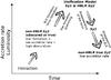 |
Fig. 4 Qualitative description of the Seyfert evolutionary scheme. |
Alternatively, it also seems possible that the true Sy2 AGN is a stand-alone phenomenon, caused by minor merging events or by secular evolution, probably initiated or re-inforced by galaxy interactions (e.g., Combes 2012). Ho (2009) showed that the low accretion rates can be supplied through local mass loss from evolved stars and Bondi accretion of hot gas, without any need for additional fueling mechanisms. No activity evolution is expected if these mechanisms cannot provide the required accretion rate to power the formation of the BLR.
In a nutshell, the current and previous studies showed that at least a fraction of non-HBLR Sy2s are probably intrinsically different from HBLR Sy2s, which in turn are probably obscured Sy1s. We argue that the non-detection of their BLR can be explained by the intrinsic lack of it, because of the low accretion rate of gas and dust onto the super-massive black hole, or alternatively, by heavy obscuration that can successfully cloak the BLR. We also argue that the existence of true Sy2 can be fitted nicely within an evolutionary scheme, where a low accretion rate is predicted at the beginning and the end of the Seyfert duty cycle. Nevertheless, we cannot rule out the possibility that some HBLR Sy2s could also be created by minor disturbances or even secular processes and that they turn off without any further evolution to other Seyfert types.
Acknowledgments
I would like to thank M. Plionis and I. Georgantopoulos for discussions and useful suggestions. The research project (PE-1145) is implemented within the framework of the Action “Supporting Postdoctoral Researchers” of the Operational Program “Education and Lifelong Learning” (Action’s Beneficiary: General Secretariat for Research and Technology), and is co-financed by the European Social Fund (ESF) and the Greek State. This research has made use of the NASA/IPAC Extragalactic Database (NED) which is operated by the Jet Propulsion Laboratory, California Institute of Technology, under contract with the National Aeronautics and Space Administration. Funding for SDSS-III has been provided by the Alfred P. Sloan Foundation, the Participating Institutions, the National Science Foundation, and the US Department of Energy Office of Science. The SDSS-III web site is http://www.sdss3.org/
References
- Akylas, A., & Georgantopoulos, I. 2009, A&A, 500, 999 [NASA ADS] [CrossRef] [EDP Sciences] [Google Scholar]
- Antonucci, R. 1993, ARA&A, 31, 473 [Google Scholar]
- Antonucci, R. 2012, Astron. Astrophys. Trans., 27, 557 [NASA ADS] [Google Scholar]
- Bahcall, N. A., Lubin, L. M., & Dorman, V. 1995, ApJ, 447, L81 [NASA ADS] [CrossRef] [Google Scholar]
- Bian, W., & Gu, Q. 2007, ApJ, 657, 159 [NASA ADS] [CrossRef] [Google Scholar]
- Bournaud, F., & Combes, F. 2002, A&A, 392, 83 [NASA ADS] [CrossRef] [EDP Sciences] [Google Scholar]
- Combes, F. 2012, J. Phys. Conf. Ser., 372, 012041 [NASA ADS] [CrossRef] [Google Scholar]
- Czerny, B., Rózańska, A., & Kuraszkiewicz, J. 2004, A&A, 428, 39 [NASA ADS] [CrossRef] [EDP Sciences] [Google Scholar]
- Deng, X.-F., He, J.-Z., Jiang, P., Song, J., & Tang, X.-X. 2008, ApJ, 677, 1040 [NASA ADS] [CrossRef] [Google Scholar]
- Denney, K. D., De Rosa, G., Croxall, K., et al. 2014, ApJ, accepted [arXiv:1404.4879] [Google Scholar]
- Dultzin-Hacyan, D., Krongold, Y., Fuentes-Guridi, I., Marziani, P., et al. 1999, ApJ, 513, L111 [NASA ADS] [CrossRef] [Google Scholar]
- Elitzur, M. 2008, Mem. Soc. Astron. It., 79, 1124 [NASA ADS] [Google Scholar]
- Elitzur, M. 2012, ApJ, 747, L33 [NASA ADS] [CrossRef] [Google Scholar]
- Elitzur, M., & Ho, L. C. 2009, ApJ, 701, L91 [NASA ADS] [CrossRef] [Google Scholar]
- Elitzur, M., & Shlosman, I. 2006, ApJ, 648, L101 [NASA ADS] [CrossRef] [Google Scholar]
- Elitzur, M., Ho, L. C., & Trump, J. R. 2014, MNRAS, 438, 3340 [NASA ADS] [CrossRef] [Google Scholar]
- Focardi, P., Zitelli, V., Marinoni, S., & Kelm, B. 2006, A&A, 456, 467 [NASA ADS] [CrossRef] [EDP Sciences] [Google Scholar]
- Gu, Q., & Huang, J. 2002, ApJ, 579, 205 [NASA ADS] [CrossRef] [Google Scholar]
- Ho, L. C. 2009, ApJ, 699, 626 [NASA ADS] [CrossRef] [Google Scholar]
- Hopkins, P. F., & Elvis, M. 2010, MNRAS, 401, 7 [NASA ADS] [CrossRef] [Google Scholar]
- Hopkins, P. F., Hernquist, L., Cox, T. J., & Kereš, D. 2008, ApJS, 175, 356 [NASA ADS] [CrossRef] [Google Scholar]
- Hunt, L. K., & Malkan, M. A. 1999, ApJ, 516, 660 [NASA ADS] [CrossRef] [Google Scholar]
- Koulouridis, E., Plionis, M., Chavushyan, V., et al. 2006a, ApJ, 639, 37 [NASA ADS] [CrossRef] [EDP Sciences] [Google Scholar]
- Koulouridis, E., Chavushyan, V., Plionis, M., et al. 2006b, ApJ, 651, 93 [NASA ADS] [CrossRef] [Google Scholar]
- Koulouridis, E., Plionis, M., Chavushyan, V., et al. 2013, A&A, 552, A135 [NASA ADS] [CrossRef] [EDP Sciences] [Google Scholar]
- Krolik, J. H. 1999, AGN: from the central black hole to the galactic environment/Julian H. Krolik (Princeton, N. J.: Princeton University Press) [Google Scholar]
- Krongold, Y., Dultzin-Hacyan, D., & Marziani, P. 2002, ApJ, 572, 169 [NASA ADS] [CrossRef] [Google Scholar]
- Krongold, Y., Nicastro, F., Elvis, M., et al. 2007, ApJ, 659, 1022 [NASA ADS] [CrossRef] [Google Scholar]
- Krongold, Y., Jiménez-Bailón, E., Santos-Lleo, M., et al. 2009, ApJ, 690, 773 [NASA ADS] [CrossRef] [Google Scholar]
- Laor, A. 2003, ApJ, 590, 86 [NASA ADS] [CrossRef] [Google Scholar]
- Levenson, N. A., Weaver, K. A., & Heckman, T. M. 2001, ApJ, 550, 230 [NASA ADS] [CrossRef] [Google Scholar]
- Lumsden, S. L., & Alexander, D. M. 2001, MNRAS, 328, L32 [NASA ADS] [CrossRef] [Google Scholar]
- Marinucci, A., Bianchi, S., Nicastro, F., Matt, G., & Goulding, A. D. 2012, ApJ, 748, 130 [NASA ADS] [CrossRef] [Google Scholar]
- Martocchia, A. 2002, Inflows, Outflows, & Reprocessing around BH, Proc. of the 5th Italian AGN, Meeting, Como, June 11–14, 34 [Google Scholar]
- Miller, J. S., & Antonucci, R. R. J. 1983, ApJ, 271, L7 [NASA ADS] [CrossRef] [Google Scholar]
- Miniutti, G., Saxton, R. D., Rodríguez-Pascual, P. M., et al. 2013, MNRAS, 433, 1764 [NASA ADS] [CrossRef] [Google Scholar]
- Nicastro, F. 2000, ApJ, 530, L65 [NASA ADS] [CrossRef] [PubMed] [Google Scholar]
- Nicastro, F., Martocchia, A., & Matt, G. 2003, ApJ, 589, L13 [NASA ADS] [CrossRef] [Google Scholar]
- Panessa, F., & Bassani, L. 2002, A&A, 394, 435 [NASA ADS] [CrossRef] [EDP Sciences] [Google Scholar]
- Patton, D. R., Grant, J. K., Simard, L., et al. 2005, AJ, 130, 2043 [NASA ADS] [CrossRef] [Google Scholar]
- Perlman, E. S., Mason, R. E., Packham, C., et al. 2007, ApJ, 663, 808 [NASA ADS] [CrossRef] [Google Scholar]
- Shu, X. W., Wang, J. X., Jiang, P., Fan, L. L., & Wang, T. G. 2007, ApJ, 657, 167 [NASA ADS] [CrossRef] [Google Scholar]
- Tommasin, S., Spinoglio, L., Malkan, M. A., & Fazio, G. 2010, ApJ, 709, 1257 [NASA ADS] [CrossRef] [Google Scholar]
- Tran, H. D. 2001, ApJ, 554, L19 [NASA ADS] [CrossRef] [Google Scholar]
- Tran, H. D. 2003, ApJ, 583, 632 [NASA ADS] [CrossRef] [Google Scholar]
- van der Wolk, G., Barthel, P. D., Peletier, R. F., & Pel, J. W. 2010, A&A, 511, A64 [NASA ADS] [CrossRef] [EDP Sciences] [Google Scholar]
- Wang, J.-M., & Zhang, E.-P. 2007, ApJ, 660, 1072 [NASA ADS] [CrossRef] [Google Scholar]
- Wang, J.-M., Du, P., Baldwin, J. A., et al. 2012, ApJ, 746, 137 [NASA ADS] [CrossRef] [Google Scholar]
- Whysong, D., & Antonucci, R. 2004, ApJ, 602, 116 [NASA ADS] [CrossRef] [Google Scholar]
- Wu, Y.-Z., Zhang, E.-P., Liang, Y.-C., Zhang, C.-M., & Zhao, Y.-H. 2011, ApJ, 730, 121 [NASA ADS] [CrossRef] [Google Scholar]
- Yu, P.-C., & Hwang, C.-Y. 2005, ApJ, 631, 720 [NASA ADS] [CrossRef] [Google Scholar]
- Yu, P.-C., Huang, K.-Y., Hwang, C.-Y., & Ohyama, Y. 2013, ApJ, 768, 30 [NASA ADS] [CrossRef] [Google Scholar]
- Zaritsky, D., Smith, R., Frenk, C., & White, S. D. M. 1997, ApJ, 478, 39 [NASA ADS] [CrossRef] [Google Scholar]
All Tables
All Figures
|
Fig. 1 Redshift (panel a)) and Morphological type (panel b)) distribution of the Sy2 samples. The solid line defines the HBLR Sy2 population, while the hatched histogram the non-HBLR. Uncertainties are 1σ Poissonian errors and they are plotted only for the HBLR Sy2s for clarity. |
| In the text | |
|
Fig. 2 Images of the merging galaxies in our samples. |
| In the text | |
|
Fig. 3 Examples of Seyferts and control sample galaxies with companions. Small companions are marked with the letter s. In the case of NGC 7582, another non-HBLR Sy2, NGC 7590 is one of the close neighbors. |
| In the text | |
|
Fig. 4 Qualitative description of the Seyfert evolutionary scheme. |
| In the text | |
Current usage metrics show cumulative count of Article Views (full-text article views including HTML views, PDF and ePub downloads, according to the available data) and Abstracts Views on Vision4Press platform.
Data correspond to usage on the plateform after 2015. The current usage metrics is available 48-96 hours after online publication and is updated daily on week days.
Initial download of the metrics may take a while.