| Issue |
A&A
Volume 570, October 2014
|
|
|---|---|---|
| Article Number | A66 | |
| Number of page(s) | 14 | |
| Section | Numerical methods and codes | |
| DOI | https://doi.org/10.1051/0004-6361/201424286 | |
| Published online | 20 October 2014 | |
Bonnsai: a Bayesian tool for comparing stars with stellar evolution models⋆
1 Argelander-Institut für Astronomie der Universität Bonn, Auf dem Hügel 71, 53121 Bonn, Germany
e-mail: This email address is being protected from spambots. You need JavaScript enabled to view it.
2 Astronomical Institute “Anton Pannekoek”, Amsterdam University, Science Park 904, 1098 XH Amsterdam, The Netherlands
3 Instituut voor Sterrenkunde, KU Leuven, Celestijnenlaan 200D, 3001 Leuven, Belgium
4 University of Vienna, Department of Astronomy, Türkenschanzstr. 17, 1180 Vienna, Austria
Received: 27 May 2014
Accepted: 2 August 2014
Abstract
Powerful telescopes equipped with multi-fibre or integral field spectrographs combined with detailed models of stellar atmospheres and automated fitting techniques allow for the analysis of large number of stars. These datasets contain a wealth of information that require new analysis techniques to bridge the gap between observations and stellar evolution models. To that end, we develop Bonnsai (BONN Stellar Astrophysics Interface), a Bayesian statistical method, that is capable of comparing all available observables simultaneously to stellar models while taking observed uncertainties and prior knowledge such as initial mass functions and distributions of stellar rotational velocities into account. Bonnsai can be used to (1) determine probability distributions of fundamental stellar parameters such as initial masses and stellar ages from complex datasets; (2) predict stellar parameters that were not yet observationally determined; and (3) test stellar models to further advance our understanding of stellar evolution. An important aspect of Bonnsai is that it singles out stars that cannot be reproduced by stellar models through χ2 hypothesis tests and posterior predictive checks. Bonnsai can be used with any set of stellar models and currently supports massive main-sequence single star models of Milky Way and Large and Small Magellanic Cloud composition. We apply our new method to mock stars to demonstrate its functionality and capabilities. In a first application, we use Bonnsai to test the stellar models of Brott et al. (2011, A&A, 530, A115) by comparing the stellar ages inferred for the primary and secondary stars of eclipsing Milky Way binaries of which the components range in mass between 4.5 and 28 M⊙. Ages are determined from dynamical masses and radii that are known to better than 3%. We show that the stellar models must include rotation because stellar radii can be increased by several percent via centrifugal forces. We find that the average age difference between the primary and secondary stars of the binaries is 0.9 ± 2.3 Myr (95% CI), i.e. that the stellar models reproduce the Milky Way binaries well. The predicted effective temperatures are in agreement for observed effective temperatures for stars cooler than 25 000 K. In hotter stars, i.e. stars earlier than B1–2V and more massive than about 10 M⊙, we find that the observed effective temperatures are on average hotter by 1.1 ± 0.3 kK (95% CI) and the bolometric luminosities are consequently larger by 0.06 ± 0.02 dex (95% CI) than predicted by the stellar models.
Key words: methods: data analysis / methods: statistical / stars: general / stars: fundamental parameters / stars: rotation / binaries: general
Bonnsai is available through a web-interface at http://www.astro.uni-bonn.de/stars/bonnsai
© ESO, 2014
1. Introduction
Stars are the building blocks of galaxies and hence the Universe. Our knowledge of their evolution is deduced from detailed comparisons of observations to theoretical models. The interface, where observations meet theory, is often provided by the Hertzsprung−Russell (HR) diagram and its relative, the colour–magnitude diagram. In an HR diagram, two surface properties of stars, the effective temperature and the luminosity, are compared to stellar evolutionary models to, e.g., determine fundamental stellar parameters like initial mass and age that are both inaccessible by observations alone and of utmost importance to modern astrophysics.
With the advent of large spectroscopic surveys1 such as the Gaia-ESO survey (Gilmore et al. 2012), SEGUE/SDSS (Yanny et al. 2009), GOSSS (Maíz Apellániz et al. 2011, 2013), RAVE (Steinmetz et al. 2006), OWN (Barbá et al. 2010), IACOB (Simón-Díaz et al. 2011; Simón-Díaz & Herrero 2014), the VLT FLAMES Survey of Massive Stars (Evans et al. 2005, 2006) and the VLT-FLAMES Tarantula Survey (Evans et al. 2011), much more is known about stars than just their positions in the HR diagram: surface abundances, surface gravities, surface rotational velocities and more. Such a wealth of information not only allows the determination of fundamental stellar parameters with high precision but also to thoroughly test and thus advance our understanding of stellar evolution. However, bridging the gap between such manifold observations and stellar models requires more sophisticated analysis techniques than simply comparing stars to models in the HR diagram because the comparison needs to be performed in a multidimensional space.
Bayesian inference is widely applied in determining cosmological parameters and offers a promising framework to infer stellar parameters from observations. Steps into this direction have been taken by Pont & Eyer (2004) and Jørgensen & Lindegren (2005) to infer stellar ages and masses from colour–magnitude diagrams. Since then, Bayesian modelling has been used by several authors to infer a wide range of stellar parameters from spectroscopy, photometry, astrometry, spectropolarimetry and also asteroseismology (e.g. da Silva et al. 2006; Takeda et al. 2007; Shkedy et al. 2007; Burnett & Binney 2010; Casagrande et al. 2011; Gruberbauer et al. 2012; Petit & Wade 2012; Bazot et al. 2012; Serenelli et al. 2013; Schönrich & Bergemann 2014). Bayesian inference is further used to derive properties of stellar ensembles such as cluster ages, mass functions and star formation histories (e.g. von Hippel et al. 2006; De Gennaro et al. 2009; van Dyk et al. 2009; Weisz et al. 2013; Walmswell et al. 2013; Dib 2014). The big advantage of a Bayesian approach is the knowledge of full probability distribution functions of stellar parameters that take observational uncertainties and prior knowledge into account.
Incorporating prior knowledge may be essential because the determination of stellar parameters can otherwise be biased (e.g. Pont & Eyer 2004). For example, the evolution of stars speeds up with time such that stars spend different amounts of time in various evolutionary phases (this even holds for stars on the main-sequence). This knowledge is typically neglected when determining stellar parameters from the position of stars in an HR diagram and may thus result in biased stellar parameters.
In this paper, we present a method that simultaneously takes all available observables, their uncertainties and prior knowledge into account to determine stellar parameters and their full probability density distributions from a set of stellar models. This method further allows us to predict yet unobserved stellar properties like rotation rates or surface abundances. By applying sophisticated goodness-of-fit tests within our Bayesian framework, we are able to securely identify stars that cannot be reproduced by the chosen stellar models which will help to improve our understanding of stellar evolution.
Initial mass ranges Mini, age ranges and initial rotational velocity ranges vini of the Bonn Milky Way (MW), Large Magellanic Cloud (LMC) and Small Magellanic Cloud (SMC) stellar models (Brott et al. 2011a; Köhler et al. 2014).
Currently, Bonnsai supports the Bonn stellar models for the Milky Way (MW), Large Magellanic Cloud (LMC) and Small Magellanic Cloud (SMC; Brott et al. 2011a; Köhler et al. 2014) with initial mass and rotational velocity ranges given in Table 1. We plan to integrate further stellar model grids in the future and make Bonnsai available through a web-interface2.
We describe the Bonnsai approach in Sect. 2 and apply it to mock stars in Sect. 3 to show its functionality and to demonstrate its capabilities. In Sect. 4 we apply Bonnsai to high-precision observations of Milky Way binaries to thoroughly test the Milky Way stellar models of Brott et al. (2011a) and conclude in Sect. 5.
2. Method
Besides the observables, there are two main ingredients in Bonnsai. On the one hand, there is the statistical method and on the other hand there are the stellar models. The statistical method uses the stellar models to derive stellar parameters from a given set of observables. In the following, we describe our statistical method (Sects. 2.1–2.4 and 2.6–2.7) and the so far implemented stellar models (Sect. 2.5).
2.1. Bayes’ theorem
Bayes’ theorem directly follows from the definition of conditional probabilities. Let P(M | D) be the conditional probability that an event M occurs given that an event D already took place, i.e. P(M | D) = P(M ∩ D) /P(D) where P(M ∩ D) is the joint probability of both events and P(D) ≠ 0 the probability for the occurrence of event D. We then arrive at Bayes’ theorem, 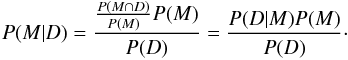 (1)In the context of Bayesian inference, M is the model parameter, D is the (observed) data and
-
P(M | D)is the posterior probability function, i.e. the probability of themodel parameter given the data,
-
P(D | M)is the likelihood, i.e. the probability of the data given the model parameter,
-
P(M)is the prior function, i.e. the probability of the model parameter,
-
and P(D) is the evidence that serves as a normalisation constant in this context because it does not depend on the model parameter.
The likelihood function per se is not a probability distribution of the model parameters that we seek to derive but it describes how likely each value of an observable is given a model. To derive the probability distribution of the model parameters, i.e. the posterior probability distribution, we apply Bayes’ theorem. In case of a uniform prior function, P(M) = const., the likelihood is the posterior probability distribution and Bayesian inference reduces to a maximum likelihood approach.
2.2. Bayesian stellar parameter determination
In the case of stellar parameter determination, the data d are now an nobs-dimensional vector containing the nobs observables like luminosities L, effective temperatures Teff, surface abundances, etc.3 The model parameter m for rotating single stars is a 4-dimensional vector consisting of the initial mass Mini, the initial rotational velocity at the equator vini, the initial chemical composition/metallicity Z and the stellar age τ. Further physics that alters the evolution of stars, like magnetic fields or duplicity, may be added to the stellar models and hence to the model parameters if needed. The model parameters uniquely map to the observables; e.g. stellar models predict luminosities, effective temperatures, etc. for given stellar initial conditions and age, m = (Mini,vini,Z,τ) → d(m) = (L,Teff,...). The reverse mapping is not always unique as evident from Fig. 2 where stellar tracks of different stars cross each other in the HRD, i.e. different model parameters, m, can predict the same observables d.
Bayes’ theorem in terms of probability density functions reads, analogously to Eq. (1), 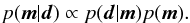 (2)The proportionality constant follows from the normalisation condition,
 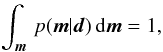 (3)where dm = dMini dvini dZ dτ. To compute p(m | d) we must define the likelihood and prior functions, which we do in the following two sections.
2.3. Likelihood function
We assume two-piece Gaussian likelihood functions to compute the posterior probability distribution according to Bayes’ theorem, Eq. (1). The probability density function of an observed quantity di with 1σ uncertainties + σp,i and −σm,i is then, ![Mathematical equation: \begin{eqnarray} p(d_{\rm i}|\vec{m})\equiv L_{i}=\frac{2}{\sqrt{2\pi}(\sigma_{m,i}+\sigma_{p,i})}\exp\left[-\frac{\left(d_{i}-d_{i}(\vec{m})\right)^{2}}{2\sigma_{i}^{2}}\right],\label{eq:pdf-gaussian} \end{eqnarray}](/articles/aa/full_html/2014/10/aa24286-14/aa24286-14-eq40.png) (4)with
(4)with 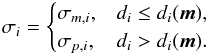 (5)If σm,i = σp,i, the likelihood function (Eq. (4)) reduces to the usual Gaussian distribution function. We assume that all nobs observables are statistically independent, i.e. they are assumed to be uncorrelated. The full likelihood function p(d | m) needed in Eq. (2) is then the product of the individual probability density functions Li of the observed data di given the model parameters m,
  (6)We further define the usual χ2,
  (7)which is useful later on.
Whenever only lower or upper limits of observables are known, we use a step function as the likelihood instead of the Gaussian function from Eq. (4). This means that all values above the lower limit and all values below the upper limit, respectively, are equally probable.
In Eq. (6) we assume that the observables are not correlated, which may lead to a loss of information. For example, effective temperatures and surface gravities that are inferred from models of stellar spectra calculated with a stellar atmosphere code are typically correlated. They are correlated in the sense that fitting a spectral line equally well with a hotter effective temperature requires a larger gravity. Such correlations are not accounted for in our current approach because the needed information is usually not published. The correlations are valuable because they contain information to constrain stellar parameters better and may thus result in smaller uncertainties. In principle correlations can readily be incorporated in our approach by including the covariance matrix in the likelihood function.
2.4. Prior functions
The prior functions contain our a priori knowledge of the model parameters m (i.e. Mini,vini,Z,τ). The prior functions do not include our knowledge of stellar evolution such as how much time stars spend in different evolutionary phases. This knowledge, that essentially is also a priori, enters our approach through the stellar models (Sect. 2.5). As for the likelihood function, we assume that the individual model parameters are independent such that the prior function splits into a product of four individual priors for the four model parameters,  (8)Our a priori knowledge of initial masses, i.e. the initial mass prior ξ(Mini), is given by the initial mass function. The initial mass function is commonly expressed as a power-law function,
  (9)with slope γ. The slope is γ = −2.35 for a Salpeter initial mass function (Salpeter 1955), meaning that lower initial masses are more probable/frequent than higher. Alternative parameterisations of the initial mass function may be used as well (see e.g. the review by Bastian et al. 2010). A uniform mass function, i.e. ξ(Mini) = const., may be used if no initial mass shall be preferred a priorly.
As an initial rotational velocity prior, θ(vini), we use observed distributions of stellar rotational velocities such as those found by Hunter et al. (2008) for O and B-type stars in the Milky Way and Magellanic Clouds. For MW and LMC stars, the observed Hunter et al. (2008) distributions follow a Gaussian distribution with mean of 100 km s-1 and standard deviation 106 km s-1 and for SMC stars a Gaussian distribution with mean 175 km s-1 and standard deviation 106 km s-1. Other observed rotational velocity distributions of OB stars are equally well suited as priors; e.g. the distributions found by Conti & Ebbets (1977), Howarth et al. (1997), Abt et al. (2002), Martayan et al. (2006, 2007), Penny & Gies (2009), Huang et al. (2010), Dufton et al. (2013) or Ramírez-Agudelo et al. (2013). We note that the observed distributions of rotational velocities are not necessarily the initial distributions that are actually required as prior function (see de Mink et al. 2013). A uniform prior, i.e. every initial rotational velocity is a priori equally probable, may be used as well.
The metallicity prior ψ(Z) has yet no influence because the metallicity is not a free model parameter in the currently supported stellar model grids. In principle, any probability distribution such as a uniform or Gaussian distribution is suited to describe a priori knowledge of the metallicity of a star under investigation. The prior can, for example, encompass knowledge of a spread in metallicity of a population of stars (e.g. Bergemann et al. 2014).
The age prior ζ(τ) is set by the star formation history of the region to which an observed star belongs. If the observed star is a member of a star cluster that formed in a single starburst, the age prior may be a Gaussian distribution with mean equal to the age of the cluster and width corresponding to the duration of the star formation process. A uniform age prior corresponds to assuming a constant star formation rate in the past such that all ages are a priori equally probable.
It is typically assumed that the inclination of a star with respect to our line-of-sight does not affect observables except for projected rotational velocities, vsini. This assumption breaks down for rapid rotators because their equators are cooler than their poles as a result of a distortion of the otherwise spherically symmetric shape of a star by the centrifugal force. The inferred effective temperature and luminosity are then a function of the inclination angle of the star towards our line-of-sight. The latter effect is beyond the scope of this paper. However, projected rotational velocities are often determined from stellar spectra. Whenever vsini measurements are compared to stellar models, we take the equatorial rotational velocities of the models and combine them with any possible orientation of the star in space, i.e. with any possible inclination angle, to derive the vsini values. By doing so, we introduce a fifth model parameter, the inclination angle i, and have to define the appropriate inclination prior, φ(i). Our assumption that the rotation axes of stars are randomly oriented in space results in inclination angles that are not equally probable. It is, for example, more likely that a star is seen equator-on (i = 90°) than pole-on (i = 0°) because the solid angle of a unit sphere, dΩ ∝ sini di, of a region around the equator is larger than that of a region around the pole. The inclination prior is then,  (10)and the full prior in Eq. (2) reads
  (11)Note that the functional form of the priors may predict non-zero probabilities for values of the model parameters that are physically meaningless. A Gaussian vini prior may result in non-zero probabilities for negative rotational velocities and a Gaussian age prior in non-zero probabilities for negative ages. Ideally, the prior functions should be properly truncated and renormalised to allow only for meaningful values of the model parameters. However, we can skip this step because the stellar model grids ensure that we only analyse physically meaningful values of the model parameters and the application of Bayes’ theorem as in Eq. (2) requires a proper renormalisation anyhow such that we can simply work with priors that are not properly normalised but describe relative differences correctly.
By default, Bonnsai assumes a Salpeter initial mass prior, uniform priors in vini, Z and age and that stellar rotation axes are randomly oriented in space.
2.5. Stellar model grids
Currently, Bonnsai supports the stellar models of Brott et al. (2011a) and Köhler et al. (2014) summarised in Table 1. Bonnsai follows a grid-based approach, i.e. we compute the posterior probability distribution by sampling models from a dense, precomputed and interpolated grid. The model grids have a resolution in initial mass of ΔMini = 0.2 M⊙, in age of Δτ = 0.02 Myr and in initial rotational velocity of Δvini = 10 km s-1. The model grids Bonn MW, LMC and SMC with their different initial mass coverage contain about 7.5, 20 and 8 million stellar models, respectively. If projected rotational velocities are matched to stellar models, we probe ten inclination angles from 0° to 90°. The model grids are computed by a linear interpolation of the stellar models of Brott et al. (2011a) and Köhler et al. (2014) with the technique described in Brott et al. (2011b).
The stellar model grids contain our (a priori) knowledge of stellar evolution. For example, the density of the stellar models is indicative of the time spent by the models in different evolutionary phases and thus ensures that this knowledge is properly taken into account in our approach.
2.6. Goodness-of-fit
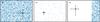 |
Fig. 1 Hypothetical model grid coverage of three observations. The resolution of the model grid is high compared to the observed uncertainties in the left panel a) and the models sample the observation well. The model grid is sparse in the middle panel b) such that the model density is not enough to resolve the 1σ uncertainties of the observations – reliable model parameters cannot be determined. In the right panel c), the models are physically unable to match the observations, i.e. the resolution of the model grid is high compared to the observed uncertainties but the models do not probe the observed region of the parameter space. |
A crucial aspect of any fitting procedure is to check the goodness of the fit (e.g. when fitting a straight line to data points that may actually follow an exponential distribution). Typically the χ2 of the fit is used as the goodness of the fit. Similarly, we have to check whether the stellar models fitted to observations are a good representation of the observations for the determined model parameters m.
As an example, consider a star in the HR diagram that lies more than 5σ bluewards of the zero-age main-sequence and is compared to non-rotating, main-sequence single star models. Our Bayesian approach presented so far would return model parameters although the models are actually unable to reach the observed position of the star in the HR diagram.
In general, the stellar models may fail to match an observation because
-
the star is not covered by the underlying stellar model grid,
-
physics is missing in the stellar models, e.g. magnetic fields, a different treatment of rotation and rotational mixing or duplicity,
-
there are problems with the calibrations of e.g. convective core overshooting, the efficiency of rotational mixing or stellar winds,
-
there are difficulties with the methods from which observables like the surface gravity are derived (e.g. stellar atmosphere models),
-
there are problematic observations like unseen binary companions that lead to misinterpretation of fluxes and spectra.
The goodness of a fit is often checked by eye. Besides a by-eye method, we develop objective and robust tests that allow us to reject the determined model parameters for a given significance level. By default, we use a significance level of α = 5% in our tests as commonly adopted in statistics.
Within our approach, stellar models might be unable to match observations not only because of the reasons given above but also because of a too low resolution of the model grid. We illustrate these cases in Fig. 1. The left panel of Fig. 1 contains a hypothetical observation including error bars and a hypothetical coverage of the observed parameter space by a stellar model grid. It is evident that the models densely cover the observation. The resolution of the model grid, i.e. the average distance between adjacent models, is small compared to the observational uncertainties. In the middle panel of Fig. 1, the stellar model grid in principle covers the observations but the model grid is sparse compared to the observational uncertainties. In order to determine reliable model parameters, the resolution of the model grid needs to be increased. Such situations are encountered whenever the observational uncertainties are so accurate that the observations including their error bars fall in between model grid points. In the right panel of Fig. 1, the model grid is dense compared to the observational uncertainties but the models are unable to match the observations. The resolution of the model grid could be infinite but the models would still not reproduce the observations. We not only want to identify situations as in Figs. 1b and c but also want to be able to distinguish between these situations.
To test whether the resolution of the stellar model grid is sufficient to determine reliable model parameters, we investigate the average spacing of those ten models that are closest to the best-fitting model. We take the nearest neighbours of each of the eleven models and compute the average differences of each observable and the average χ2 of these pairs. We define as our resolution criterion that the average differences are less than one fifth of the corresponding 1σ uncertainties. This ensures that there are about ten models within 1σ of each observable and that we know how significant the χ2 of the best fitting model is with respect to the resolution of the stellar model grid.
Once it is ensured that the resolution of the model grid is sufficient, we test whether the stellar models are able to match the observations. One straightforward way to judge the goodness of the estimated parameters is to do a classical χ2-hypothesis test (Pearson’s χ2-hypothesis test). The χ2 of the best-fitting model,  , is compared to the maximum allowable
  for a given significance level α, where the maximum allowable is such that the integrated probability of the χ2-distribution for
  is equal to the significance level. This means that there is a probability less than α that
  for the best-fitting stellar model. The χ2-distribution is defined by the degrees of freedom which, in our case, is given by the number of observables. If some observables are dependent on each other, i.e. if some observables can be derived from others as is the case for surface gravity, mass and radius or luminosity, effective temperature and radius, the χ2-test gives a too large , i.e. the test is performed with an effectively smaller significance level.
The χ2-test only incorporates the best-fitting stellar model. In a Bayesian analysis there are not only the model parameters of the best-fitting stellar model but the full posterior probability distribution of the model parameters that do not necessarily peak at the best-fitting model parameters. We make use of this by conducting a posterior predictive check. The idea is to compare the predictions of the stellar models for the estimated model parameters to the observations to check whether the predictions are in agreement with the observations. If they are not in agreement, the estimated model parameters and hence the stellar models cannot reproduce/replicate the observations. In Bayesian statistics, the predictions of the models for the observables are called replicated observables, drep, and are computed from the full posterior probability distribution, p(m | d), 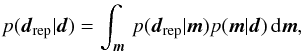 (12)where p(drep | d) is the probability distribution of the replicated observables (given the original observables) and p(drep | m) is the probability of the replicated parameters drep given a stellar model with parameters m (i.e. p(drep | m) consists, in our case, of delta-functions). From the likelihood function (Eq. (6)) and the posterior predictive probability distribution of the replicated observables (Eq. (12)), we compute the probability distributions p(Δdi | d) of the differences between the replicated and original observables, Δdi ≡ drep,i − di. If the stellar models can reproduce the observations, the differences between replicated and original observables have to be consistent with being zero. We define the differences to be consistent with zero if the integrated probabilities for Δdi> 0 and Δdi< 0 are both larger than the significance level α for all observables di, i = 1...nobs, i.e.
 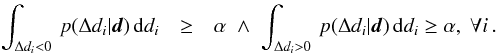 (13)In other words, we say that the stellar models cannot reproduce the observations if the probability that the model prediction of any quantity is larger or smaller than the observational value is ≥95% (≥1 − α with α = 5%).
Besides these automated and objective tests, we check the coverage of the observed parameter space graphically in diagrams similar to the illustrations in Fig. 1. We place one dot for each stellar model together with the observables and their uncertainties into two-dimensional projections of the parameter space of the observables. This results in nobs(nobs + 1)/2 projections for nobs observables from which the resolution can be assessed as well as whether the models are able to reproduce the observations (see Fig. 6 below for an example).
2.7. Our new approach in practice
In practice we perform the following steps:
-
1.
We select all stellar models from a database (model grid) that arewithin 5σi of all observables. The pre-selectionreduces the parameter space of the stellar models
 that needs to be scanned and thus accelerates the analysis.
 -
2.
We scan the pre-selected model parameter space and compute for each model the posterior probability according to Eq. (2). The posterior probability consists of the likelihood from Eq. (6) and a weighting factor that gives the probability of finding a stellar model with the given model parameters, m. The weighting factor consists of two contributions: first, it takes into account the prior function from Eq. (11) factoring in our a priori knowledge about the probability of finding a particular stellar model and, second, the volume ΔV = ΔMini Δvini ΔZ Δτ Δi that a particular stellar model covers in the model grid. The latter allows us to use non-equidistant model grids.
-
3.
We renormalise the posterior probabilities such that Eq. (3) is fulfilled and create 1D and 2D probability functions/maps for the model parameters m by marginalisation, i.e. by projecting the posterior probability distribution onto, e.g., the Mini axis or into the vini − Mini plane. Additionally we use Eq. (12) to derive probability functions/maps of any stellar parameter to e.g. predict yet unobserved surface nitrogen abundances of the stellar models for the estimated model parameters.
-
4.
The resolution and goodness-of-fit tests are conducted.
-
5.
The 1D probability functions are analysed to compute the mean, median and mode including their 1σ uncertainties.
3. Testing Bonnsai with mock stars
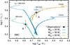 |
Fig. 2 Position of the mock stars, Star A and Star B, in the HR diagram compared to rotating and non-rotating stellar evolutionary models of Brott et al. (2011a) of SMC composition. The dots on the stellar tracks are equally spaced by 0.25 Myr. |
In the following sections, we apply Bonnsai to the two SMC mock stars, Star A and Star B, whose position in the HR diagram is shown in Fig. 2 together with SMC stellar evolutionary models of Brott et al. (2011a). We analyse Star A in Sect. 3.1 and Star B in 3.2.
3.1. Mock Star A
Mock Star A has an effective temperature of Teff = 43 200 ± 2500 K and a luminosity of log L/L⊙ = 5.74 ± 0.10 (Fig. 2). Its position in the HR diagram is equally well matched by an initially rapidly (424 km s-1) rotating 35 M⊙ star and a non-rotating 50 M⊙ star. The initial rapid rotator starts out evolving chemically homogeneously. Rotationally induced mixing brings helium, synthesized by hydrogen burning in the stellar core, to the surface which in turn reduces the electron scattering opacity. Therefore, it stays more compact, evolves towards hotter effective temperatures and becomes more luminous than its non-rotating counterpart. It is tempting to conclude that both evolutionary scenarios are equally likely because both fit the position of the star in the HR diagram equally well. However, this is a biased view that does not take a priori knowledge of stars and stellar evolution into account – we can actually exclude the rapidly rotating 35 M⊙ star with more than 95% confidence as we show below.
There are two different sources of a priori knowledge, namely that of (a) the model parameters, i.e. what we know about the initial mass, age, initial rotational velocity and metallicity of the star before analysing it; and (b) stellar evolution. The former enters our approach through the prior functions (Sect. 2.4) and the latter through the stellar models used to compute the likelihood (Sect. 2.3). From the point of view of the prior functions, 35 M⊙ models are preferred over 50 M⊙ because of the IMF, but moderately rotating 50 M⊙ models over rapidly rotating 35 M⊙ stars because of observed distributions of stellar rotation rates. From the point of view of stellar models, the 50 M⊙ track is preferred because the 50 M⊙ model spends more time at the observed position in the HR diagram than the 35 M⊙ model that is close to the end of its main-sequence evolution where evolution is more rapid. The 50 M⊙ models are also preferred because there are many models of that mass with different initial rotational velocities that reach the observed position in the HR diagram while there is only a narrow range of initial rotation rates of 35 M⊙ models that match the observations.
The a priori knowledge allows us to quantify how likely both models are. Only additional observables that are sensitive to rotation enable us to fully resolve the degenerate situation.
In the following, we match Star A against the SMC models of Brott et al. (2011a), choose a Salpeter mass function as initial mass prior and a uniform age prior. We vary the initial rotational velocity prior and use an additional constraint on the surface helium abundance to show their influence on the posterior probability distributions. The resolution test, the χ2-hypothesis test and the posterior predictive checks are passed in all cases. We present a summary of our test cases in Table 2.
3.1.1. Uniform initial rotational velocity prior
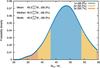 |
Fig. 3 Initial mass posterior probability distribution of mock Star A from Fig. 2. The shaded regions give the 1σ, 2σ and 3σ confidence regions. |
At first we apply a uniform vini prior, i.e. we assume that all initial rotational velocities are a priori equally probable. The resulting posterior probability distribution of the initial mass is shown in Fig. 3 as a histogram with a binwidth of 0.2 M⊙. The mean, median and mode are given with their 1σ uncertainties (the confidence level is indicated in parentheses). The most probable initial mass is  , the most probable age is
  and the initial rotational velocity is unconstrained, i.e. its posterior probability distribution is uniform until it steeply drops-off at vini ≳ 400 km s-1 (left panel in Fig. 4). The likelihood of a 35 M⊙ star is small. It is only within the 3σ uncertainty despite the Salpeter IMF prior that prefers lower initial masses. The reason why the 50 M⊙ models are favoured over rapidly rotating 35 M⊙ stars is best seen in the vini − Mini plane of the posterior probability distribution in Fig. 4. Only a small subset of 35 M⊙ fast rotators, those with vini ≳ 400 km s-1, reach the observed position in the HR diagram and thus contribute to the posterior probability distribution of the initial mass in Fig. 3. The range of initial rotational velocities of stars around 50 M⊙ that contribute to the posterior probability is much larger and has thus a correspondingly larger weight (Fig. 4). In conclusion, both the 35 and 50 M⊙ models reproduce the position in the HR diagram equally well but it is much more likely that the star is a 50 M⊙ star: 35 M⊙ models are excluded with a confidence of more than 97.5%.
As evident from this example, the (marginalised) posterior distributions contain a wealth of information that is partly lost when looking only at the summary statistics, e.g. the mode and confidence levels. We therefore encourage all Bonnsai users to first inspect the marginalised posterior probability distributions before making use of the summary statistics.
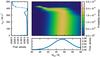 |
Fig. 4 Posterior probability map of the vini–Mini plane (middle panel) adopting a Salpeter initial mass function as Mini prior and a uniform prior for vini. One dimensional posterior probability distributions of initial rotational velocities vini (left panel) and initial masses Mini (bottom panel) are also given. |
3.1.2. Gaussian initial rotational velocity prior
We now change the initial rotational velocity prior to show its influence on the posterior probability. We use the observationally determined distribution of rotational velocities of SMC early B-type stars from Hunter et al. (2008) as a prior. This distribution is well approximated by a Gaussian with mean ⟨vrot⟩ = 175 km s-1 and standard deviation σv = 106 km s-1. The distribution disfavours slow (≲100 km s-1) and fast rotators (≳250 km s-1) compared to the uniform vini prior. This is reflected in the vini − Mini plane of the posterior probability in Fig. 5. Slow and fast rotators are now less likely than before with the uniform vini prior. The posterior probability function of the initial mass and age are however nearly unaffected: the most likely initial mass is  . Fast-rotating 35 M⊙ stars are now even less likely because the chosen prior favours moderate rotators. The most likely initial rotational velocity now is
  , i.e. it follows the vini prior both in the mean value and the uncertainty because it is otherwise unconstrained in this example (Sect. 3.1.1).
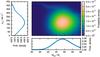 |
Fig. 5 As Fig. 4 but using as vini prior the observed distribution of rotational velocities of SMC early B-type stars from Hunter et al. (2008). |
3.1.3. Including the surface helium mass fraction
The degeneracy in HR diagrams (Fig. 2) that arises from rotational mixing can be removed if observables that are sensitive to rotation are incorporated in the analysis. We use observed surface helium mass fractions, Y, as an additional constraint to demonstrate this (the initial mass fraction of the SMC models of Brott et al. 2011a is Yini = 0.2515). The surface helium abundance is sensitive to rotation as rotational mixing brings more helium to the surface the faster the star rotates.
A surface helium mass fraction of Y ≤ 0.3 rules out rapid rotators (≳350 km s-1) because their surfaces are enriched in helium to more than 30% in mass. When assuming a uniform vini prior, the most likely initial mass is  , i.e. slightly larger than before because rapid rotators are totally excluded and not only suppressed as in Sect. 3.1.2 without the additional surface helium mass fraction constraint and a Gaussian vini prior.
Contrarily, a surface helium mass fraction of Y ≥ 0.4 allows only for rapid rotators because stars rotating initially slower than about 350 km s-1 do not enrich their surfaces by more than 40% in helium at the observed position in the HR diagram. So even assuming that the initial rotational velocities are distributed according to Hunter et al. (2008) – a Gaussian distribution that highly suppresses rapid rotators – results in a most likely initial rotational velocity of  . Consequently, the most likely initial mass is lower, namely
  , and the most likely age is older, namely
  .
.
3.2. Mock Star B
Next we consider the mock Star B with a luminosity of log L/L⊙ = 5.45 ± 0.10, effective temperature Teff = 60 200 ± 3500 K and surface helium mass fraction Y = 0.25 ± 0.05 (Fig. 2). Only rapid rotators evolving chemically homogeneously reach the position of Star B in the HR diagram. Main-sequence SMC models of Brott et al. (2011a) at that position in the HR diagram are significantly enriched with helium at their surface,  (Yini = 0.2515). Contrarily, our mock Star B has the initial helium abundance, thus the stellar models cannot reproduce the star. In the following, we show how such situations are robustly identified within Bonnsai using the goodness-of-fit criteria from Sect. 2.6 after ensuring that the resolution of the model grid is sufficiently high.
3.2.1. Resolution and χ2–hypothesis test
In Fig. 6 we show the stellar model coverage of the parameter space of the observables. As described in Sect. 2.7, stellar models are chosen within 5σ of the observations from the model database, i.e. the luminosities of the stellar models are in the range log L/L⊙ = 4.95 − 5.95, the effective temperatures in Teff = 42 700 − 77 700 K and the surface helium mass fractions in Y = 0.00 − 0.50. There are no stellar models in the direct vicinity of the observation because only those stars that are highly enriched with helium at their surface () are found at the observed position in the HR diagram.
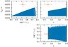 |
Fig. 6 Coverage of the projected parameter space of the observables of our mock Star B (Sect. 3.2). One dot for each stellar model and the observables including their 1σ uncertainties are plotted. |
Projections like those in Fig. 6 can not be readily used as a criterion to accept a Bonnsai solution but should only be used as an analysis tool. The best-fitting stellar model might be far away from the observation (e.g. 5σ) while all projections homogeneously and densely cover the observation. This can happen whenever the stellar models cover the surface of the nobs-dimensional parameter space but not the inside. The projections are then homogeneously filled with stellar models but the closest model is still far away from the observation.
In the present case, the automatic resolution test as described in Sect. 2.6 confirms the visual impression of Fig. 6 that the resolution of the stellar model grid is sufficiently high, i.e. that the observables, including their error bars, do not fall between model grid points. An insufficient resolution as a reason for not finding stellar models close to the observation can be excluded and the results of our analysis do not suffer from resolution problems.
The maximum allowable χ2 for a significance level α = 5% and three degrees of freedom is  . The χ2 of the best-fitting stellar model is
  . We therefore conclude that the stellar models are unable to explain the observables with a confidence of ≥95%.
3.2.2. Posterior predictive check
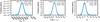 |
Fig. 7 Probability distributions of the differences of the replicated and original observables of our mock Star B (left panel: effective temperature; middle panel: luminosity; right panel: surface helium mass fraction). The stellar models predict effective temperatures that are significantly cooler than the observations and are thus not able to reproduce the star. |
In a Bayesian analysis we not only test the best fitting model but use the full posterior probability distribution to evaluate the goodness of the fit. From the obtained model parameters, we compute the model predictions, i.e. the probability distributions, of the observables effective temperature, luminosity and surface helium mass fraction, that are called replicated observables. The probability distributions of the replicated observables are then compared to those of the original observations, i.e. to the individual likelihood functions, Li (Eq. (4)), to check whether the predictions of the models for the obtained model parameters are in agreement with the observations. To that end, we compute the probability distributions of the differences of replicated and original observables which we show in Fig. 7. We find that the effective temperatures deviate by ΔTeff = Teff,rep − Teff,obs = −11 921 ± 3735 K such that the replicated effective temperatures are cooler than the observed temperatures in more than 99% of the cases – the stellar models can clearly not reproduce the observations. The replicated luminosities and surface helium mass fractions are in agreement with the observations (Δlog L/L⊙ = 0.10 ± 0.13 and ΔY = −0.01 ± 0.06; Fig. 7).
4. Testing stellar evolution models with eclipsing binaries
In the previous sections we show that our new method provides stellar parameters including robust uncertainties and reliably identifies stars that cannot be reproduced by stellar models when applied to mock data (Sect. 3). One of the primary goals of Bonnsai is to test the physics in stellar models by matching the models to observations in a statistically sound way. For that it is necessary to have well determined stellar parameters that – ideally – do not rely on extensive modelling and/or calibrations. Eclipsing, double-lined spectroscopic binaries and interferometric observations of single stars are prime candidates for this purpose.
We use Bonnsai in combination with precise measurements of stellar masses and radii of Milky Way binaries (Torres et al. 2010) to test the Milky Way stellar models of Brott et al. (2011a). The stellar masses and radii of the Milky Way binary components are determined from observed radial-velocity curves and light curves. We call masses and radii determined in this way dynamical masses and dynamical radii. The surface gravities, log g, follow directly from the measured dynamical masses and radii. Additionally, the stellar bolometric luminosities follow from the Stefan-Boltzmann law if the effective temperatures are known as well. The latter typically rely on multi-band photometry and calibrations, individual spectra or a comparison of the spectral energy distributions obtained by narrow band filters with stellar atmosphere models (spectro-photometry).
Observed stellar parameters of those Milky Way binaries in the sample of Torres et al. (2010) that we use to test Bonnsai and the stellar models of Brott et al. (2011a).
The Torres et al. (2010) sample of Milky Way binary stars is an updated extension of the sample of Andersen (1991). All binary stars are analysed homogeneously and dynamical masses and radii are known to better than 3%. We work with a subsample of the Torres et al. (2010) sample, namely with all stars that are within the mass range covered by our Milky Way stellar models. We extend the published stellar models of Brott et al. (2011a) by unpublished ones down to 4 M⊙ to increase our binary sample size by three. We describe our method to test the stellar models in Sect. 4.1, explain why stellar rotation needs to be accounted for in Sect. 4.2, present the results of our test in Sect. 4.3 and compare effective temperatures and bolometric luminosities predicted by the models to the observed values in Sect. 4.4.
4.1. Description of our test
The primary and secondary stars in binaries can be assumed to be coeval. We use this condition to test stellar models by comparing the ages determined individually for the primary and secondary star of each binary. The ages inferred for the primary and secondary star may deviate if the physics and calibrations of the stellar models are not accurate. This or a similar test is often applied to binaries in order to test stellar evolution and investigate convective core overshooting (see e.g. Andersen 1991; Schroder et al. 1997; Pols et al. 1997; Clausen et al. 2010; Torres et al. 2010, 2014, and references therein).
In case of observed dynamical masses and radii, the stellar ages are constrained through the time dependence of stellar radii because the masses of stars in the binary sample of Torres et al. (2010) hardly change with time. However, stellar radii, R, depend not only on age but on a variety of parameters,  such as – in addition to age τ – mass M, rotational velocity vrot, metallicity Z and the treatment of convection, indicated here by the convective mixing length parameter αML and the convective core overshooting length lov. The mixing length parameter, αML, plays only a minor role in the hot stars considered here. Besides the dynamically measured masses and radii, we use, if available, the observed projected rotational velocities vsini to determine stellar ages (Table 3). The parameters radius, mass and rotational velocity are fixed within their uncertainties by the observations and the derived stellar ages depend on the remaining parameters. That is, our test probes the chemical composition (metallicity) and the implementation and calibration of rotation and convection in the stellar models. The metallicities are also known to a certain degree because the binary sample consists of Milky Way stars.
Because of the precise observations, we use denser stellar model grids than those available by default in the Bonnsai web-service. With the higher resolution our resolution test, the χ2-hypothesis test and our posterior predictive check are passed by all stars.
Our test loses significance if the stars in a binary have very similar masses and radii because the ages derived for such similar stars have to be the same no matter which stellar models and calibrations are used. In the following we therefore cite the mass ratios q of secondary to primary star to easily spot binaries with similar stellar components.
We compare the stars in the binaries to stellar evolutionary models of single stars. This assumption is good as long as the past evolution of the stars is not influenced significantly by binary interactions. Past mass transfer episodes are not expected to have occurred in our binary sample because all the stars are on the main-sequence and presently do not fill their Roche lobes. Tidal interactions, however, have influenced the binaries and affect stellar radii in two ways: (1) tides spin stars up or down which consequently changes their radii by rotational mixing and centrifugal forces; (2) tides dissipate energy inside stars, thereby giving rise to an additional energy source that might increase stellar radii. All binary stars in Torres et al. (2010) whose radii are larger than about 25% of the orbital separation are circularised, implying that the stellar rotation periods are synchronised with the orbital periods because synchronisation is expected to precede circularisation. Once the binaries are synchronised and circularised, no torques act on the stars and tides no longer influence the evolution until stellar evolution either changes the spin period of the stars or the orbit by e.g. wind mass loss such that tides are active again. We have to keep this in mind when comparing the observations to single star models that do not take tidal evolution into account.
4.2. The role of rotation in Milky Way binaries
The stars with known rotation rates in our sample have projected rotational velocities vsini between 20 and 230 km s-1. The associated centrifugal forces lead to larger stellar radii. Within the Roche model, we approximate by how much stellar radii change as a function of rotational velocity. The Roche potential ψ(r,ϑ) of a star with mass M rotating with frequency Ω = 2π/Ps (Ps being the rotation period) is given by  (14)where r is the radial distance and ϑ the polar angle, G is the gravitational constant and mr is the mass within radius r. The Roche potential evaluated at the stellar pole (r = Rp, ϑ = 0) and at the stellar equator (r = Re, ϑ = π/ 2) are equal because the stellar surface is on an equipotential. Equating ψ(R,0) = ψ(R,π/ 2),
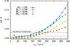 |
Fig. 8 Relative radius difference of zero-age, rotating and non-rotating stellar models from Brott et al. (2011a) as a function of initial rotational velocity vini and initial stellar mass Mini. |
introducing the break-up or critical rotational frequency  (i.e. Keplerian frequency at the equator) and Γ = Ω/Ωcrit, we have for the relative difference of the equatorial and polar radius
  (15)The polar radius Rp is not explicitly affected by rotation and hence it can be viewed as the radius of a star in absence of rotation (centrifugal forces do not act in the direction of the rotation axis). Hence, Eq. (15) provides an estimate of the relative increase in equatorial radius of stars rotating with a fraction Γ of critical rotation. The equatorial radius increases by 3% if the star rotates with about 25% of critical rotation.
In Fig. 8 we show the increase of the equatorial stellar radii of rotating zero-age main-sequence stars compared to non-rotating stars (ΔR/R ≡ [Rrot − Rnon − rot] /Rnon − rot) as a function of initial rotational velocity vini and initial stellar mass Mini. Stars that have masses ≤10 M⊙ and rotate with about 100 km s-1 have radii increased by about 1%. The radii are increased by more than 3% if stars rotate faster than about 200 km s-1. Given that dynamical radii in Torres et al. (2010) are all known to better than 3% and often to about 1%, our estimates show that, at such accuracies, rotation has to be considered to accurately test the stellar models.
4.3. The ages of primary and secondary stars
We determine stellar parameters of the binary stars from dynamical masses, dynamical radii and projected rotational velocities (Table 3). The latter are not available for the binaries V1034 Sco, V478 Cyg, CW Cep and DI Her, so we determine their stellar parameters from their dynamical masses and radii alone. Our determined initial mass, age, initial rotational velocity, effective temperature, surface gravity and luminosity are summarised in Table 4 including their (mostly) 1σ uncertainties (see caption of Table 4). We also indicate the approximate fractional main-sequence age, τ/τMS, of the stars in 5% steps. The main-sequence lifetimes, τMS, of the stellar models are determined from the obtained initial mass and initial rotational velocity.
The ages τA and τB of the primary and secondary star of binaries from Table 4 are plotted against each other in Fig. 9. If the stellar models were a perfect representation of the observed stars, the ages of the binary components should agree within their 1σ uncertainties in 68.3%, i.e. in 12–13 of the 18 cases. A first inspection reveals that the ages of the binary components agree well within their uncertainties, except for one >6σ outlier, V1388 Ori. We do not have an explanation for the discrepant ages of V1388 Ori. Perhaps the metallicity of this star differs from solar, which may induce an age difference. Alternatively, the formation history of the system may be peculiar.
Stellar radii grow only slowly in the beginning of a stellar life but more quickly when approaching the end of the main-sequence evolution. For example, a non-rotating 10 M⊙ Milky Way star of Brott et al. (2011a) has increased its radius by about 40% at half of its main-sequence life but by about 230% towards its end. Hence, the accuracy with which ages can be determined from dynamical masses and radii depends strongly on the fractional main-sequence age of stars and becomes better the more evolved a star is. Because of this the age of CV Vel (τ/τMS ≈ 60%) is determined to about 3% whereas the age of DI Her (τ/τMS ≈ 5 − 10%) is only determined to about 50–60%, despite an accuracy of 1–2% in stellar masses and radii in both cases.
We quantify the age differences, Δτ = τA − τB, of the primary and secondary stars and evaluate whether the age differences deviate significantly from zero. As noted in Sect. 4.1, our test loses significance if both stars in a binary are too similar, therefore we exclude those binaries from our analysis that have mass ratios larger than 0.97. This holds for the binaries V478 Cyg, CV Vel and MU Cas (the largest mass ratio of the remaining binaries, namely that of EM Car and DW Car, is 0.94). We also exclude the outlier V1388 Ori. The mean, relative age difference of the remaining 14 binaries is ⟨Δτ/δΔτ⟩ = −0.09 ± 0.43 (95% CI), where δΔτ are the 1σ uncertainties of the age differences Δτ and the uncertainty ±0.43 is the 95% confidence interval of the standard error  with σ = 0.82 being the standard deviation of the relative age differences and n = 14 the sample size. Further χ2- and t-tests confirm, with a confidence level of 95% (p-values of 0.85 and 0.47, respectively), that the age differences are consistent with being zero (mean age difference ⟨Δτ⟩ = 0.9 ± 2.3 Myr, 95% CI).
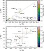 |
Fig. 9 Ages of primary (τA) and secondary (τB) stars determined from dynamical masses, dynamical radii and (if available) projected rotational velocities vsini. The colour coding indicates the mass ratios of secondary (MB) to primary (MA) stars. Squares and filled circles show binaries for which vsini measurements are available and are lacking to derive stellar ages, respectively. The bottom panel is a zoom into the age range 0 − 12.5 Myr of the top panel. |
Convective core overshooting influences stellar radii most strongly towards the end of the main-sequence evolution and has little influence on unevolved stars. A test with a 5 M⊙ Milky Way star with an overshooting of 0.5 pressure scale heights compared to no overshooting shows that the stellar radii differ by less than 3–4% for fractional main-sequence ages younger than 30–40%. The maximum radii reached during the main-sequence evolution at fractional main-sequence ages of 98–99% differ by 53%, i.e. the model with overshooting has a radius larger by a factor of 1/(1 − 0.53) ≈ 2.1. In the following we assume that stars with fractional main-sequence ages less than 35% can be viewed as being unaffected by convective core overshooting. Hence, by restricting the test to those binaries in which the primary stars have fractional main-sequence ages younger than about 35%, i.e. to the binaries V3903 Sgr, V578 Mon, DW Car, QX Car, AG Per, DI Her and V760 Sco, we mainly probe the combination of metallicity and rotation in our models. The mean, relative age difference of this subsample of binary stars is ⟨Δτ/δΔτ⟩ = 0.14 ± 0.73 (95% CI) and χ2- and t-tests confirm, with a 95% confidence level (p-values of 0.54 and 0.30, respectively), that the age differences are consistent with zero (mean age difference ⟨Δτ⟩ = 2.4 ± 4.2 Myr, 95% CI). We find no significant evidence for a correlation between the inferred age- and observed mass-differences of the binary stars.
Iron abundances, total metallicities ZBrott as given in Brott et al. (2011a) and the corresponding metallicities Zκ of the opacity tables used in the Brott et al. (2011a) models.
Our test with the subsample of binaries that are not expected to be influenced by convective core overshooting shows that the Milky Way stellar models of Brott et al. (2011a), with their metallicity and calibration of rotation, reproduce the massive (4.5 − 28 M⊙) Milky Way binaries in the sample of Torres et al. (2010). This might come as a surprise because the models are computed for a metallicity of Z = 0.0088, which is small compared to current estimates of the metallicity of the Sun (Z⊙ = 0.014 − 0.020; Grevesse & Sauval 1998; Asplund et al. 2009). Though the total metallicity in the models of Brott et al. (2011a) is rather low compared to that of the Sun, the iron abundance is not. The opacities in the models are interpolated linearly in the iron abundances from standard OPAL opacity tables (Iglesias & Rogers 1996). The iron abundance in the Brott et al. (2011a) models is log (Fe/H) + 12 = 7.40 (Table 5) which is close to the iron abundance of log (Fe/H) + 12 ≈ 7.50 in the Sun (e.g. Grevesse & Sauval 1998; Asplund et al. 2009), hence the structures of stars from Brott et al. (2011a) follow those of stars with a solar-like composition.
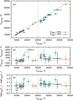 |
Fig. 10 Comparison of observed Teff,obs with predicted effective temperatures Teff,theo for stars in our Milky Way binary sample and its consequence for stellar luminosities (cf. Tables 3 and 4). Panel a) shows a direct comparison of the observed and predicted effective temperatures, panel b) the differences of these temperatures ΔTeff = Teff,obs − Teff,theo as a function of observed effective temperature and panel c) the resulting differences of the observed and predicted bolometric luminosities Δlog L = log Lobs − log Ltheo. The squares show stars with fractional main-sequence ages τ/τMS younger than 35% (models not influenced by core overshooting) while the filled circles represent τ/τMS> 35% (models influenced by core overshooting). |
Rotation increases the stellar radii at a level which is comparable to that of the uncertainties of the radii (Fig. 8) and thus must be accounted for when testing stellar models (Sect. 4.2). Rotating stars are larger than non-rotating stars and hence reach the observed radii earlier in their evolution. Stellar ages inferred from rotating stellar models are therefore systematically younger than those inferred from non-rotating stellar models. To quantify the systematic age shift, we determine the ages of all 36 stars in our sample using only the non-rotating Milky Way stellar models of Brott et al. (2011a). We find a mean, relative age difference of  (95% CI) where the error is again the 95% confidence interval of the standard error. The ages inferred from rotating stellar models are younger than those from non-rotating models for all stars.
4.4. Effective temperatures and bolometric luminosities
The effective temperatures of stars in the Milky Way binary sample of Torres et al. (2010) are independent observables. The effective temperatures mainly follow from multi-band photometry, calibrations with respect to spectral types and colours, individual stellar spectra and spectral energy distributions. Once the effective temperatures are known, the bolometric luminosities are derived using the Stefan Boltzmann law and the dynamical radii. Besides determining, e.g., stellar ages, we further compute the posterior probability distributions of the effective temperatures of stars from the measured dynamical masses, radii and projected rotational velocities. We then compare the predictions of the stellar models in terms of effective temperatures and bolometric luminosities to the observations (Fig. 10). In the following we exclude V1388 Ori because our stellar models cannot reproduce this binary.
We find that the observed effective temperatures and hence bolometric luminosities of our stars are in agreement with the predictions of the stellar models of Brott et al. (2011a) for observed effective temperatures Teff,obs< 25 000 K (⟨ΔTeff⟩ = 133 ± 188 K, 95% CI; ⟨Δlog L/L⊙⟩ = 0.01 ± 0.02 dex, 95% CI). However, the observed effective temperatures are on average hotter by 1062 ± 330 K (95% CI) and the bolometric luminosities are consequently larger by 0.06 ± 0.02 dex (95% CI) for Teff,obs> 25 000 K than predicted by the stellar models.
The convective core overshooting in our models is not responsible for the discrepant effective temperatures for Teff,obs> 25 000 K. The average difference between observed and predicted effective temperatures of those stars whose radii are not influenced yet by convective core overshooting (stars with fractional main-sequence ages τ/τMS ≤ 35%) is −88 ± 377 K (95% CI) for Teff,obs< 25 000 K and 758 ± 371 K (95% CI) for Teff,obs> 25 000 K. The average differences in effective temperatures of stars expected to be influenced by core overshooting (τ/τMS> 35%) are 183 ± 496 K (95% CI) for Teff,obs< 25 000 K and 1213 ± 461 K (95% CI) for Teff,obs> 25 000 K.
The cause of the discrepant effective temperatures in stars hotter than 25 000 K, i.e. earlier than B1–2V or more massive than about 10 M⊙, is unknown. We speculate that the discrepancy is partly explained by calibrations becoming less accurate for more massive stars. To understand this, we recall how such calibrations are obtained in practice. In cool stars, fundamental effective temperatures, i.e. that do not rely on any modelling, can be determined from bolometric fluxes Fbol that are derived from spectral energy distributions and from interferometric measurements of stellar angular diameters θ (![Mathematical equation: \hbox{$F_{\mathrm{bol}}=[\theta/2]^{2}\sigma T_{\mathrm{eff}}^{4}$}](/articles/aa/full_html/2014/10/aa24286-14/aa24286-14-eq657.png) , where σ is the Stefan Boltzmann constant). Such fundamental measurements of effective temperatures are more complicated and practically impossible in hot stars because they radiate a substantial fraction of their light in the ultraviolet (UV) that is difficult to access observationally (most UV space telescopes cannot observe shortward of 90 nm which is the wavelength at which a black body of Teff ≈ 32 000 K radiates most of its energy). Bolometric fluxes of hot stars are therefore difficult to measure directly and stellar atmosphere models are often used to predict the flux in the far UV. Instead of this procedure, model atmosphere computations are applied to infer effective temperatures directly from spectra and to establish the calibrations with spectral types and colours. The derived effective temperatures are therefore dependent on the treatment of, for instance, non-LTE effects, line blanketing, and stellar winds. Compared to these model atmospheres, the boundary conditions of the stellar structure models are relatively simple and this may be a cause of the discrepant effective temperatures.
, where σ is the Stefan Boltzmann constant). Such fundamental measurements of effective temperatures are more complicated and practically impossible in hot stars because they radiate a substantial fraction of their light in the ultraviolet (UV) that is difficult to access observationally (most UV space telescopes cannot observe shortward of 90 nm which is the wavelength at which a black body of Teff ≈ 32 000 K radiates most of its energy). Bolometric fluxes of hot stars are therefore difficult to measure directly and stellar atmosphere models are often used to predict the flux in the far UV. Instead of this procedure, model atmosphere computations are applied to infer effective temperatures directly from spectra and to establish the calibrations with spectral types and colours. The derived effective temperatures are therefore dependent on the treatment of, for instance, non-LTE effects, line blanketing, and stellar winds. Compared to these model atmospheres, the boundary conditions of the stellar structure models are relatively simple and this may be a cause of the discrepant effective temperatures.
5. Conclusions
With the advent of large stellar surveys on powerful telescopes and advances in analysis techniques of stellar atmospheres more is known about stars than just their position in the Hertzsprung−Russell (HR) diagram – rotation rates, surface gravities and abundances of many stars are derived. Therefore, the comparison of observations to theoretical stellar models to infer essential quantities like initial mass or stellar age and to test stellar models has to be done in a multidimensional space spanned by all available observables. To that end we develop Bonnsai4, a Bayesian method that allows us to match all available observables simultaneously to stellar models taking the observed uncertainties and prior knowledge like mass functions properly into account. Our method is based on Bayes’ theorem from which we determine full (posterior) probability distributions of the stellar parameters such as initial mass and stellar age. The probability distributions are analysed to infer the model parameters including robust uncertainties. Bonnsai securely identifies cases where the observed stars are not reproduced by the underlying stellar models through χ2-hypothesis tests and posterior predictive checks. We test Bonnsai with mock data to demonstrate its functionality and to show its capabilities.
We apply Bonnsai to the massive star subsample (≥4 M⊙) of the Milky Way binaries of Torres et al. (2010). The masses and radii of the binaries are known to better than 3%. For each of the 36 binary components in this sample, we determine the initial masses, ages, fractional main-sequence ages and initial rotational velocities from the observed masses, radii and, if available, projected rotational velocities applying the stellar models of Brott et al. (2011a). We find that the Milky Way stellar models of Brott et al. (2011a) result in stellar ages for 17 binaries that are equal within the uncertainties. There is no statistically significant age difference (95% confidence level). We find that Bonnsai, in combination with the Milky Way stellar models of Brott et al. (2011a), can not fit one binary, V1388 Ori, for which the ages of both stars differ by >6σ.
We further compare the effective temperatures predicted by the stellar models to the observed effective temperatures. The predicted effective temperatures agree with the observed within their uncertainties for observed effective temperatures Teff,obs ≤ 25 000 K. The observed effective temperatures are hotter by 1063 ± 330 K (95% CI) than the effective temperatures of the models when Teff,obs> 25 000 K. The cause of this discrepancy is unknown but may be connected to the complexities of the atmospheres of hot OB stars. The systematically hotter temperatures result in stars being brighter by 0.06 ± 0.02 dex (95% CI) compared to the stellar models.
The Bonnsai approach is flexible and can be easily extended and applied to different fields in stellar astrophysics. In its current form, Bonnsai allows us to compare observed stellar surface properties to models of massive, rotating, main-sequence single stars. Asteroseismology nowadays offers a look into the interiors of stars. By extending the stellar models to asteroseismic observables, Bonnsai could make use of these observables as well to constrain stellar models. Similarly, Bonnsai can be extended to also match pre main-sequence stars, post main-sequence stars, low mass stars, binary stars, stars of varying metallicities etc. to corresponding stellar models. Our statistical approach also enables the calibration of stellar parameters such as convective core overshooting including robust uncertainties and to analyse whole stellar populations to, e.g., unravel initial mass functions and star formation histories in a statistically sound way while properly taking observable uncertainties into account.
Sloan Digital Sky Survey (SDSS), Sloan Extension for Galactic Understanding and Exploration (SEGUE/SDSS), Galactic O Star Spectroscopic Survey (GOSSS), RAdial Velocity Experiment (RAVE), Spectroscopic Survey of Galactic O and WN stars (OWN), Instituto de Astrofísica de Canarias OB star survey (IACOB).
What we call observables are actually not observables but quantities derived from observations, e.g. from modelling of stellar spectra. For clarity we nevertheless use the phrase observables in this paper.
The Bonnsai web-service is available at http://www.astro.uni-bonn.de/stars/bonnsai
Acknowledgments
We thank Selma de Mink, Luca Fossati, Jonathan Mackey, Oscar Ramírez-Agudelo, Hugues Sana, Richard Stancliffe, Frank Tramper and the VFTS consortium for stimulating discussions, constructive feedback and testing the Bonnsai web-service. In particular, we thank Claudia McCain for her help regarding the web-service. We further thank an anonymous referee for constructive suggestions that helped to improve the presentation of the paper. F.R.N.S. acknowledges the fellowship granted by the Bonn-Cologne Graduate School of Physics and Astronomy (BCGS) through the excellence initiative of the German Research Foundation (DFG). R.G.I. and H.H.B.L. thank the Alexander von Humboldt foundation.
References
- Abt, H. A., Levato, H., & Grosso, M. 2002, ApJ, 573, 359 [NASA ADS] [CrossRef] [Google Scholar]
- Andersen, J. 1991, A&AR, 3, 91 [Google Scholar]
- Asplund, M., Grevesse, N., Sauval, A. J., & Scott, P. 2009, ARA&A, 47, 481 [NASA ADS] [CrossRef] [Google Scholar]
- Barbá, R. H., Gamen, R., Arias, J. I., et al. 2010, in Rev. Mex. Astron. Astrofis. Conf. Ser., 38, 30 [Google Scholar]
- Bastian, N., Covey, K. R., & Meyer, M. R. 2010, ARA&A, 48, 339 [NASA ADS] [CrossRef] [Google Scholar]
- Bazot, M., Bourguignon, S., & Christensen-Dalsgaard, J. 2012, MNRAS, 427, 1847 [NASA ADS] [CrossRef] [Google Scholar]
- Bergemann, M., Ruchti, G. R., Serenelli, A., et al. 2014, A&A, 565, A89 [NASA ADS] [CrossRef] [EDP Sciences] [Google Scholar]
- Brott, I., de Mink, S. E., Cantiello, M., et al. 2011a, A&A, 530, A115 [NASA ADS] [CrossRef] [EDP Sciences] [Google Scholar]
- Brott, I., Evans, C. J., Hunter, I., et al. 2011b, A&A, 530, A116 [NASA ADS] [CrossRef] [EDP Sciences] [Google Scholar]
- Burnett, B., & Binney, J. 2010, MNRAS, 407, 339 [NASA ADS] [CrossRef] [Google Scholar]
- Casagrande, L., Schönrich, R., Asplund, M., et al. 2011, A&A, 530, A138 [NASA ADS] [CrossRef] [EDP Sciences] [Google Scholar]
- Clausen, J. V., Frandsen, S., Bruntt, H., et al. 2010, A&A, 516, A42 [NASA ADS] [CrossRef] [EDP Sciences] [Google Scholar]
- Conti, P. S., & Ebbets, D. 1977, ApJ, 213, 438 [NASA ADS] [CrossRef] [Google Scholar]
- da Silva, L., Girardi, L., Pasquini, L., et al. 2006, A&A, 458, 609 [NASA ADS] [CrossRef] [EDP Sciences] [Google Scholar]
- De Gennaro, S., von Hippel, T., Jefferys, W. H., et al. 2009, ApJ, 696, 12 [NASA ADS] [CrossRef] [Google Scholar]
- de Mink, S. E., Langer, N., Izzard, R. G., Sana, H., & de Koter, A. 2013, ApJ, 764, 166 [NASA ADS] [CrossRef] [Google Scholar]
- Dib, S. 2014, MNRAS, 444, 1957 [NASA ADS] [CrossRef] [MathSciNet] [Google Scholar]
- Evans, C. J., Lennon, D. J., Smartt, S. J., & Trundle, C. 2006, A&A, 456, 623 [NASA ADS] [CrossRef] [EDP Sciences] [Google Scholar]
- Dufton, P. L., Langer, N., Dunstall, P. R., et al. 2013, A&A, 550, A109 [NASA ADS] [CrossRef] [EDP Sciences] [Google Scholar]
- Evans, C. J., Smartt, S. J., Lee, J.-K., et al. 2005, A&A, 437, 467 [NASA ADS] [CrossRef] [EDP Sciences] [Google Scholar]
- Evans, C. J., Taylor, W. D., Hénault-Brunet, V., et al. 2011, A&A, 530, A108 [NASA ADS] [CrossRef] [EDP Sciences] [Google Scholar]
- Gilmore, G., Randich, S., Asplund, M., et al. 2012, The Messenger, 147, 25 [NASA ADS] [Google Scholar]
- Grevesse, N., & Sauval, A. J. 1998, Space Sci. Rev., 85, 161 [NASA ADS] [CrossRef] [Google Scholar]
- Gruberbauer, M., Guenther, D. B., & Kallinger, T. 2012, ApJ, 749, 109 [NASA ADS] [CrossRef] [Google Scholar]
- Howarth, I. D., Siebert, K. W., Hussain, G. A. J., & Prinja, R. K. 1997, MNRAS, 284, 265 [NASA ADS] [CrossRef] [Google Scholar]
- Huang, W., Gies, D. R., & McSwain, M. V. 2010, ApJ, 722, 605 [NASA ADS] [CrossRef] [Google Scholar]
- Hunter, I., Lennon, D. J., Dufton, P. L., et al. 2008, A&A, 479, 541 [NASA ADS] [CrossRef] [EDP Sciences] [Google Scholar]
- Iglesias, C. A., & Rogers, F. J. 1996, ApJ, 464, 943 [NASA ADS] [CrossRef] [Google Scholar]
- Jørgensen, B. R., & Lindegren, L. 2005, A&A, 436, 127 [NASA ADS] [CrossRef] [EDP Sciences] [Google Scholar]
- Köhler, K., Langer, N., de Koter, A., et al. 2014, A&A, submitted [Google Scholar]
- Maíz Apellániz, J., Sota, A., Walborn, N. R., et al. 2011, in Highlights of Spanish Astrophysics VI, eds. M. R. Zapatero Osorio, J. Gorgas, J. Maíz Apellániz, J. R. Pardo, & A. Gil de Paz, 467 [Google Scholar]
- Maíz Apellániz, J., Sota, A., Morrell, N. I., et al. 2013, in Massive Stars: From alpha to Omega [Google Scholar]
- Martayan, C., Frémat, Y., Hubert, A.-M., et al. 2006, A&A, 452, 273 [NASA ADS] [CrossRef] [EDP Sciences] [Google Scholar]
- Martayan, C., Frémat, Y., Hubert, A.-M., et al. 2007, A&A, 462, 683 [NASA ADS] [CrossRef] [EDP Sciences] [Google Scholar]
- Penny, L. R., & Gies, D. R. 2009, ApJ, 700, 844 [NASA ADS] [CrossRef] [Google Scholar]
- Petit, V., & Wade, G. A. 2012, MNRAS, 420, 773 [NASA ADS] [CrossRef] [Google Scholar]
- Pols, O. R., Tout, C. A., Schroder, K.-P., Eggleton, P. P., & Manners, J. 1997, MNRAS, 289, 869 [NASA ADS] [CrossRef] [Google Scholar]
- Pont, F., & Eyer, L. 2004, MNRAS, 351, 487 [NASA ADS] [CrossRef] [Google Scholar]
- Ramírez-Agudelo, O. H., Simón-Díaz, S., Sana, H., et al. 2013, A&A, 560, A29 [NASA ADS] [CrossRef] [EDP Sciences] [Google Scholar]
- Salpeter, E. E. 1955, ApJ, 121, 161 [Google Scholar]
- Schönrich, R., & Bergemann, M. 2014, MNRAS, 443, 698 [NASA ADS] [CrossRef] [Google Scholar]
- Schroder, K.-P., Pols, O. R., & Eggleton, P. P. 1997, MNRAS, 285, 696 [NASA ADS] [CrossRef] [Google Scholar]
- Serenelli, A. M., Bergemann, M., Ruchti, G., & Casagrande, L. 2013, MNRAS, 429, 3645 [NASA ADS] [CrossRef] [Google Scholar]
- Shkedy, Z., Decin, L., Molenberghs, G., & Aerts, C. 2007, MNRAS, 377, 120 [NASA ADS] [CrossRef] [Google Scholar]
- Simón-Díaz, S., & Herrero, A. 2014, A&A, 562, A135 [NASA ADS] [CrossRef] [EDP Sciences] [Google Scholar]
- Simón-Díaz, S., Castro, N., Garcia, M., Herrero, A., & Markova, N. 2011, Bull. Soc. Roy. Sci. Liege, 80, 514 [Google Scholar]
- Steinmetz, M., Zwitter, T., Siebert, A., et al. 2006, AJ, 132, 1645 [NASA ADS] [CrossRef] [Google Scholar]
- Takeda, G., Ford, E. B., Sills, A., et al. 2007, ApJS, 168, 297 [NASA ADS] [CrossRef] [Google Scholar]
- Torres, G., Andersen, J., & Giménez, A. 2010, A&ARv, 18, 67 [Google Scholar]
- Torres, G., Vaz, L. P. R., Sandberg Lacy, C. H., & Claret, A. 2014, AJ, 147, 36 [NASA ADS] [CrossRef] [Google Scholar]
- van Dyk, D. A., Degennaro, S., Stein, N., Jefferys, W. H., & von Hippel, T. 2009, Ann. Appl. Statist., 3, 117 [Google Scholar]
- von Hippel, T., Jefferys, W. H., Scott, J., et al. 2006, ApJ, 645, 1436 [NASA ADS] [CrossRef] [Google Scholar]
- Walmswell, J. J., Eldridge, J. J., Brewer, B. J., & Tout, C. A. 2013, MNRAS, 435, 2171 [NASA ADS] [CrossRef] [Google Scholar]
- Weisz, D. R., Fouesneau, M., Hogg, D. W., et al. 2013, ApJ, 762, 123 [NASA ADS] [CrossRef] [Google Scholar]
- Yanny, B., Rockosi, C., Newberg, H. J., et al. 2009, AJ, 137, 4377 [NASA ADS] [CrossRef] [Google Scholar]
All Tables
Initial mass ranges Mini, age ranges and initial rotational velocity ranges vini of the Bonn Milky Way (MW), Large Magellanic Cloud (LMC) and Small Magellanic Cloud (SMC) stellar models (Brott et al. 2011a; Köhler et al. 2014).
Observed stellar parameters of those Milky Way binaries in the sample of Torres et al. (2010) that we use to test Bonnsai and the stellar models of Brott et al. (2011a).
Iron abundances, total metallicities ZBrott as given in Brott et al. (2011a) and the corresponding metallicities Zκ of the opacity tables used in the Brott et al. (2011a) models.
All Figures
|
Fig. 1 Hypothetical model grid coverage of three observations. The resolution of the model grid is high compared to the observed uncertainties in the left panel a) and the models sample the observation well. The model grid is sparse in the middle panel b) such that the model density is not enough to resolve the 1σ uncertainties of the observations – reliable model parameters cannot be determined. In the right panel c), the models are physically unable to match the observations, i.e. the resolution of the model grid is high compared to the observed uncertainties but the models do not probe the observed region of the parameter space. |
| In the text | |
|
Fig. 2 Position of the mock stars, Star A and Star B, in the HR diagram compared to rotating and non-rotating stellar evolutionary models of Brott et al. (2011a) of SMC composition. The dots on the stellar tracks are equally spaced by 0.25 Myr. |
| In the text | |
|
Fig. 3 Initial mass posterior probability distribution of mock Star A from Fig. 2. The shaded regions give the 1σ, 2σ and 3σ confidence regions. |
| In the text | |
|
Fig. 4 Posterior probability map of the vini–Mini plane (middle panel) adopting a Salpeter initial mass function as Mini prior and a uniform prior for vini. One dimensional posterior probability distributions of initial rotational velocities vini (left panel) and initial masses Mini (bottom panel) are also given. |
| In the text | |
|
Fig. 5 As Fig. 4 but using as vini prior the observed distribution of rotational velocities of SMC early B-type stars from Hunter et al. (2008). |
| In the text | |
|
Fig. 6 Coverage of the projected parameter space of the observables of our mock Star B (Sect. 3.2). One dot for each stellar model and the observables including their 1σ uncertainties are plotted. |
| In the text | |
|
Fig. 7 Probability distributions of the differences of the replicated and original observables of our mock Star B (left panel: effective temperature; middle panel: luminosity; right panel: surface helium mass fraction). The stellar models predict effective temperatures that are significantly cooler than the observations and are thus not able to reproduce the star. |
| In the text | |
|
Fig. 8 Relative radius difference of zero-age, rotating and non-rotating stellar models from Brott et al. (2011a) as a function of initial rotational velocity vini and initial stellar mass Mini. |
| In the text | |
|
Fig. 9 Ages of primary (τA) and secondary (τB) stars determined from dynamical masses, dynamical radii and (if available) projected rotational velocities vsini. The colour coding indicates the mass ratios of secondary (MB) to primary (MA) stars. Squares and filled circles show binaries for which vsini measurements are available and are lacking to derive stellar ages, respectively. The bottom panel is a zoom into the age range 0 − 12.5 Myr of the top panel. |
| In the text | |
|
Fig. 10 Comparison of observed Teff,obs with predicted effective temperatures Teff,theo for stars in our Milky Way binary sample and its consequence for stellar luminosities (cf. Tables 3 and 4). Panel a) shows a direct comparison of the observed and predicted effective temperatures, panel b) the differences of these temperatures ΔTeff = Teff,obs − Teff,theo as a function of observed effective temperature and panel c) the resulting differences of the observed and predicted bolometric luminosities Δlog L = log Lobs − log Ltheo. The squares show stars with fractional main-sequence ages τ/τMS younger than 35% (models not influenced by core overshooting) while the filled circles represent τ/τMS> 35% (models influenced by core overshooting). |
| In the text | |
Current usage metrics show cumulative count of Article Views (full-text article views including HTML views, PDF and ePub downloads, according to the available data) and Abstracts Views on Vision4Press platform.
Data correspond to usage on the plateform after 2015. The current usage metrics is available 48-96 hours after online publication and is updated daily on week days.
Initial download of the metrics may take a while.