| Issue |
A&A
Volume 570, October 2014
|
|
|---|---|---|
| Article Number | A111 | |
| Number of page(s) | 22 | |
| Section | Astrophysical processes | |
| DOI | https://doi.org/10.1051/0004-6361/201424083 | |
| Published online | 03 November 2014 | |
Relativistic magnetic reconnection in collisionless ion-electron plasmas explored with particle-in-cell simulations
1
École Normale Supérieure, Lyon, CRAL, UMR CNRS 5574, Université de
Lyon,
69364
Lyon Cedex 07,
France
e-mail:
This email address is being protected from spambots. You need JavaScript enabled to view it.
2
CSCS Lugano, via Trevano 131, 6900
Lugano,
Switzerland
Received: 28 April 2014
Accepted: 27 July 2014
Abstract
Magnetic reconnection is a leading mechanism for magnetic energy conversion and high-energy non-thermal particle production in a variety of high-energy astrophysical objects, including ones with relativistic ion-electron plasmas (e.g., microquasars or AGNs), a regime where first principle studies are scarce. We present 2D particle-in-cell (PIC) simulations of low β ion-electron plasmas under relativistic conditions, i.e., with inflow magnetic energy exceeding the plasma restmass energy. We identify outstanding properties: (i) For relativistic inflow magnetizations (here 10 ≤ σe ≤ 360), the reconnection outflows are dominated by thermal agitation instead of bulk kinetic energy. (ii) At high inflow electron magnetization (σe ≥ 80), the reconnection electric field is sustained more by bulk inertia than by thermal inertia. It challenges the thermal-inertia paradigm and its implications. (iii) The inflows feature sharp transitions at the entrance of the diffusion zones. These are not shocks but results from particle ballistic motions, all bouncing at the same location, provided that the thermal velocity in the inflow is far lower than the inflow E × B bulk velocity. (iv) Island centers are magnetically isolated from the rest of the flow and can present a density depletion at their center. (v) The reconnection rates are slightly higher than in non-relativistic studies. They are best normalized by the inflow relativistic Alfvén speed projected in the outflow direction, which then leads to rates in a close range (0.14–0.25), thus allowing for an easy estimation of the reconnection electric field.
Key words: plasmas / magnetic reconnection / relativistic processes / methods: numerical / instabilities
© ESO, 2014
1. Introduction
Magnetic reconnection has been the focus of extended studies since its first introduction by Giovanelli (1947, 1948) to explain the sudden release of energy in solar flares. The term itself was coined by Dungey (1958). It is now the key ingredient for theories of coronal heating, solar flares and jets, and coronal mass ejections in the Sun (Priest 1987), of magnetic storms and substorms in the Earth magnetosphere (Paschmann et al. 2013), and for the behavior of fusion plasmas with, for instance, the sawtooth oscillation in tokamaks (Biskamp 2000). Space physics proves that magnetic reconnection can quickly convert magnetic energy into kinetic energies (bulk flow, heat, non-thermal particles) with fast variability and high efficiency.
Such attributes made it attractive for high-energy astrophysics to explain, for example, radiation (Romanova & Lovelace 1992) and flares (Giannios et al. 2009) in active galactic nuclei (AGNs) jets or in gamma-ray bursts (Lyutikov 2006a; Lazar et al. 2009), the heating of AGN and microquasar coronae and associated flares (Di Matteo 1998; Merloni & Fabian 2001; Goodman & Uzdensky 2008; Reis & Miller 2013), the flat radio spectra from galactic nuclei and AGNs (Birk et al. 2001), the heating of the lobes of giant radio galaxies (Kronberg et al. 2004), the σ-paradox and particle acceleration at pulsar wind termination shocks (Kirk & Skjæraasen 2003; Pétri & Lyubarsky 2007; Sironi & Spitkovsky 2011), GeV flares from the Crab nebula (Cerutti et al. 2012a,b, 2013), transient outflow production in microquasars and quasars (de Gouveia dal Pino & Lazarian 2005; de Gouveia Dal Pino et al. 2010; Kowal et al. 2011; McKinney et al. 2012; Dexter et al. 2014), gamma-ray burst outflows and non-thermal emissions (Drenkhahn & Spruit 2002; McKinney & Uzdensky 2012), X-ray flashes (Drenkhahn & Spruit 2002), soft gamma-ray repeaters (Lyutikov 2006b; Uzdensky 2011), flares in double pulsar systems (Lyutikov & Lazarian 2013), or energy extraction in the ergosphere of black holes (Koide & Arai 2008).
As pointed out by Uzdensky (2006), magnetic reconnection is of dynamical importance in any environment both where magnetic fields dominate the energy budget, so that the energy transfer can have dynamical and observable consequences, and where the rates of reconnection are fast. The latter is known to hold both in collisionless plasmas (Birn et al. 2001) and in collisional plasmas, either via turbulence (Lazarian & Vishniac 1999; Lapenta & Lazarian 2012; Lazarian et al. 2012), or via plasmoid induced reconnection (Uzdensky et al. 2010; Zanotti & Dumbser 2011; Loureiro et al. 2007, 2012).
Many of these environments are collisionless (Ji & Daughton 2011), so that fast reconnection must be triggered and sustained by non-ideal terms other than collisional ones, which implies kinetic processes on scales close to the electron inertial length or Larmor radius, with particles largely out of equilibrium and possibly comprising high-energy tails. These non-ideal terms can be linked to particle inertia and wave-particle resonant interactions or to finite Larmor radius effects in magnetic field gradients. Simulation studies thus require full kinetic codes, such as Vlasov solvers or particle-in-cell algorithms.
Most of the above environments are also relativistic, either because of relativistic velocities (bulk flows or currents) or because the thermal kinetic energy and/or the magnetic energy density exceeds the restmass energy of the particles. The latter translates into an inflow magnetization larger than unity,  , with s denoting ions or electrons. This magnetic energy can be transferred to the particles, and because it is greater than the particles restmass, relativistic particles are expected. The relation h0,out,sΓout,s = 1 + σin,s, with h0,out,s the enthalpy and Γout,s the bulk Lorentz factor of the reconnection outflow (see Sect. 3.4, Eq. (11)), indeed shows that either relativistic temperatures (h0,out,s> 1) or relativistic bulk velocities (Γout,s> 1) are obtained for the outflows. The relevant magnetization is thus not that of the plasma, which is low because of the ion mass, but that of each species taken individually.
Studies of relativistic reconnection are scarcer than their non-relativistic counterparts (for the latter, see the reviews by Birn & Priest 2007; Treumann & Baumjohann 2013), and they mainly deal with pair plasmas. For relativistic pair plasmas, they include analytical works (Tenbarge et al. 2010; Kojima et al. 2011) and Sweet-Parker-like analysis (Blackman & Field 1994; Lyutikov & Uzdensky 2003; Lyubarsky 2005), 2D MHD simulations (Watanabe & Yokoyama 2006; Zenitani et al. 2011a; Takahashi et al. 2011; Zanotti & Dumbser 2011; Takamoto 2013; Baty et al. 2013), two-fluid simulations (Zenitani et al. 2009a,b), test-particle simulations (Bulanov & Sasorov 1976; Romanova & Lovelace 1992; Larrabee et al. 2003; Cerutti et al. 2012a), 1D PIC simulations (Pétri & Lyubarsky 2007), 2D PIC simulations (Jaroschek et al. 2008; Sironi & Spitkovsky 2011; Bessho & Bhattacharjee 2012; Cerutti et al. 2012b, 2013; Zenitani & Hoshino 2001, 2005a, 2007, 2008; Zenitani & Hesse 2008), and 3D PIC simulations (Zenitani & Hoshino 2008, 2005b; Sironi & Spitkovsky 2011, 2014; Kagan et al. 2013; Cerutti et al. 2014). Relativistic reconnection in ion-electron plasmas has been studied less. We find a test-particle simulation (Romanova & Lovelace 1992), a resolution of the diffusion equation (Birk et al. 2001), and a discussion by Sakai et al. (2002) in a 2D PIC simulation of laser fusion beams.
The focus of the present work is on relativistic reconnection, as compared to non-relativistic studies, and on ion-electron plasmas, as compared to pair plasmas. Our goals are to carve out aspects that are particular to this regime, to shed light on the underlying physical causes, and to ultimately put our findings in the, admittedly speculative, larger astrophysical context of microquasar and AGN disk coronae and magnetospheres, and of other possible environments with ion-electron relativistic plasmas. Part of our results are also of interest for pair plasmas and for non-relativistic cases.
In Sect. 2 we describe the simulation setup and parameters. Section 3 presents the results of simulations with antiparallel asymptotic magnetic fields. We investigate the structure of the two-scale diffusion region in Sect. 3.2, and explain why we see sharp transitions at the entrance of this region. Next, we turn to the relativistic Ohm’s law. In non-relativistic reconnection, non-ideal terms are dominated by thermal inertia, i.e., by the divergence of off-diagonal elements of the pressure tensor. There are, however, PIC studies (see references of Sect. 3.3) suggesting that for relativistic reconnection, thermal inertia can be dominated by bulk inertia. In Sect. 3.3 we show that this is the case in our simulations with large inflow magnetization. We demonstrate in Sect. 3.8 that this is to be expected on the basis of an analytical model. Concerning the reconnection outflows, mass and energy conservation imply that relativistic inflow magnetization results in relativistic temperatures and/or relativistic bulk velocities in the outflows, but say nothing about the balance between the two. In Sect. 3.4 we show that in our simulations, thermal energy largely dominates the bulk kinetic energy. We demonstrate analytically in Sect. 3.8 that this is to be expected for large inflow magnetization, under the assumption that thermal inertia significantly contributes in Ohm’s law. This is an important question that has observational consequences. In Sect. 3.5 we detail the structure of the magnetic islands and of their central density dips and isolated centers. Section 3.6 studies the reconnection electric field. The relevant normalization is non-trivial for relativistic setups, and we propose to use the relativistic Alfvén speed in the inflow, which leads to rates in a close range. Section 4 highlights differences resulting from the presence of a guide magnetic field. We summarize and conclude our work in Sect. 5 and discuss applications to astrophysical objects.
2. Problem setup
2.1. Description of the relativistic Harris equilibrium
We use the explicit particle-in-cell code Apar-T, presented and tested in Melzani et al. (2013). Broadly speaking, it is a parallel electromagnetic relativistic 3D PIC code with a staggered grid, where the fields are integrated via Faraday and Maxwell-Ampère equations, currents computed by a charge conserving volume weighting (CIC), and fields interpolated accordingly.
The simulations start from a Harris equilibrium, which is a solution of the Vlasov-Maxwell system. The magnetic field is  (see Figs. 1 or 2 for axis orientation), and is sustained by a population of electrons and ions of equal number density ncs(x) = ncs(0) / cosh2(x/L) (cs stands for current sheet), flowing with bulk velocities Ue and Ui = −Ue in the ± y directions. We denote the associated Lorentz factors by Γe and Γi. Each species follows a Maxwell-Jüttner distribution (Eq. (A.1)) of normalized temperature Θs = 1 /μs = Ts/msc2.
We derived the equilibrium relations for relativistic temperatures and current drift speeds, as well as for arbitrary ion to electron mass ratios and temperature ratios, in Melzani et al. (2013). Details specific to the present application can be found in Appendix A. The equilibrium depends on the ratio ωce/ωpe, with ωpe = (ncs(0)e2/ (ϵ0me))1 / 2 the electron plasma pulsation defined with the lab-frame number density ncs(0) (not including background particles), and ωce = eB0/me the electron cyclotron pulsation in the asymptotic magnetic field (not including the guide field, e> 0). Our simulations are, however, not loaded exactly with the equilibrium values, but with a temperature and current speed uniformly in excess of ~ 10% in order to shorten the otherwise rather long stable phase.
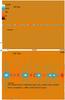 |
Fig. 1 Electron number density in the whole simulation domain, at two different times. From run ωce/ωpe = 3, |
We also set a background plasma of number density (for electrons or for ions) nbg and of temperature Tbg,e for electrons and Tbg,i for ions. Finally, a guide magnetic field is sometimes considered, i.e., a uniform component  . Adding the background plasma or the guide field does not change the Harris equilibrium.
2.2. Magnetization and energy fluxes
There are several ways to characterize the magnetization of the configuration. The ratio ωce/ωpe has no direct physical meaning and is mostly used as a simulation label. The magnetization  of the background plasma species s is the ratio of the energy flux in the reconnecting magnetic field to that in the particles (restmass, thermal, bulk). The electromagnetic energy flux is the Poynting flux. Far from the current sheet, it reads as
 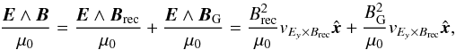 (1)where
  and vEy × Brec = Ey/Brec. This splitting of the energy flux into two contributions, one from the magnetic field that will reconnect, the other from the guide field that will mostly be compressed, is possible only if the electric field is normal to B, which is indeed the case in the ideal outer area because of the tendency of the plasma to screen parallel electric fields. For the particles, the energy flux of species s is (Eq. (B.9))
  (2)with nlab,s the particle number density in the lab frame (=Γs times that in the comoving frame), ⟨ ·⟩ s denoting an average over momentum of the distribution function, ms the particle mass,
  their bulk velocity, Γs the associated Lorentz factor, and h0,s their comoving enthalpy (drawn in Fig. B.1 for a thermal distribution). All in all, the magnetization of species s is
  (3)with
  the magnetization of the plasma without taking temperature effects and relativistic bulk motion into account:
  (4)If
(4)If  exceeds unity, then it is possible to pass to the particles an amount of energy from the reconnecting field that exceeds their restmass; i.e., it is possible to obtain relativistic particles. We do not include the guide field
  in the definition of the magnetization because it is mostly compressed and does not transfer energy to the particles.
 |
Fig. 2 Zoom around a X point showing various fluid quantities. From run ωce/ωpe = 3, |


Finally, the total magnetization of the plasma is 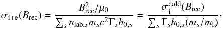 (5)In the inflow part of our simulations, we have h0,i ~ 1, h0,e < 2.6, and mi = 25me for the range of background temperatures considered here, so that the particle energy flux is largely dominated by the restmass energy flux of the ions, which is
  , and has no temperature dependence. We thus have
  , and σi + e is not a good representative of the electron physics and of the possibility that they are relativistically magnetized. The inflow magnetizations in our simulations are presented in Table 2.
2.3. Alfvén velocities
We give the definitions of the Alfvén speeds that will be used to discuss the normalization of the reconnection electric field in Sect. 3.6. They are reported in Table 2. The Alfvén velocity in the inflow plasma, far from the current sheet, is expressed in the comoving plasma frame and is, respectively in the non-relativistic and relativistic cases, 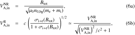 where σi + e(Btot) is to be expressed in the comoving frame (Eq. (5) with nlab,s = n0,bg the comoving density and Γs = 1), and where
  . For the relativistic expression 6b, the first equality is general and derived from the relativistic ideal MHD description (Gedalin 1993), while the second holds only because mi ≫ me so that the total enthalpy is dominated by the ion contribution. When there is a guide magnetic field, we show in Sect. 4.3 that it is relevant to project the Alfvén speed into the direction of the reconnecting magnetic field (
 ), i.e., to consider
  with tanθ = BG/B0.
A hybrid Alfvén speed is often defined in the literature as depending on the asymptotic magnetic field (without the guide field) and on the comoving density at the center of the current sheet: 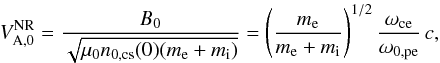 (7)where a subscript 0 indicates a comoving quantity. Its relativistic generalization is denoted by
  and is obtained with Eq. (6b) but with parameters of the plasma at the center of the current sheet in the magnetization.
2.4. Simulation parameters and resolution tests
The physical parameters of the main simulations are given in Tables 1 and 2. We consider a mass ratio mi/me = 25, except for one simulation with pairs. The background plasma number density is nbg = 0.1ncs(0) or 0.3ncs(0). Its temperature is varied between Tbg = 1.5 × 10⁷K (2.5 × 10⁻³mec2) and 3 × 10⁹K (0.5 mec2). The magnetization depends on the ratio ωce/ωpe = 1, 3, or 6, leading to inflow magnetizations between 10 and 260 for electrons, or 0.4 and 14 for ions. The current sheet is either of initial halfwidth L = 0.5di = 2.5de or L = 1di in the ωce/ωpe = 6 case, with de, di the inertial lengths defined at current sheet center. We stress that for relativistic temperatures the sheet width in terms of Larmor radii will not be the same for simulations with different ωce/ωpe (Eq. (A.5)); see L/rce in Table 1.
The numerical resolution is set by the number of cells nx per electron inertial length de, by the number of timesteps nt per electron plasma period 2π/ωpe, and by the number of computer particles (the so-called superparticles) per cell ρsp. The quantities de, ωpe, and ρsp are defined at t = 0 at the center of the current sheet, where the particle density is highest. For the simulations of Table 2, we take nx = 9 and nt = 150 (250 for ωce/ωpe = 6). We checked with a simulation with twice this resolution (ωce/ωpe = 3, nx = 18, nt = 250) that all of the presented results are not affected1.
Parameters of the current sheet.
Physical input parameters of the simulations and resulting magnetizations of the background plasma.
Concerning the number of superparticles per cell, the simulations of Table 2 use ρsp = 1820 (1090 for nbg/ncs(0) = 0.3). For the case nbg/ncs(0) = 0.1, this corresponds to 1650 electron and ion superparticles per cell for the plasma of the current sheet and to 170 for the background plasma. The density profile of the current sheet plasma is set by changing the number of superparticles per cell when going away from the center. We stressed in Melzani et al. (2013, 2014a) that because of their low numbers of superparticles per cell when compared to real plasmas, PIC simulations present high levels of collisionality. One should thus ensure that collisionless kinetic processes remain faster than collisional effects (e.g., for thermalization), essentially by taking a large enough number ΛPIC of superparticles per Debye sphere. For example, with Θe = 2.4 the electron Debye length is 20 cells large, and we have initially at the center of the current sheet: ΛPIC ~ 364 × 20 × 20 = 7.3 × 10⁵ superparticles. For a background plasma with Tbg = 2 × 10⁸ K: ΛPIC = 133. We performed a simulation identical to the one with ωce/ωpe = 3, nbg/ncs(0) = 0.1, Tbg = 2 × 10⁸ K, but with half the superparticles, and found no change in the results. It shows that the main simulations use large enough ρsp.
Boundaries are periodic along z and y. At the top and bottom x boundaries, we use reflective boundaries; i.e., we place a perfectly conducting wall that reflects waves and particles. The number of cells for the standard simulations is 4100 × 6144. The length along y is of no dynamical importance, and the dimensions correspond to a 2D simulation with 455 initial electron inertial lengths along x and 683 along z, typically with 4 × 10⁹ superparticles. It takes 70 Tpe for light waves to start from the current sheet, reflect at the ± x boundaries, and come back to the sheet. for, respectively, simulations with ωce/ωpe = 1, 3, 6. The light travel time in the z direction is longer. Except for run ωce/ωpe = 1, all the analyses presented here are for shorter times and are thus not affected by boundaries. To check this, we performed a larger simulation with 8000 × 10 240 cells (i.e., 888 × 1138 initial electron inertial length) for the case ωce/ωpe = 3, nbg/ncs(0) = 0.1, Tbg = 2 × 10⁸ K, with the same nt, nx, ρsp. The corresponding light-crossing time is now  . All the results are the same, which shows that we do not suffer from boundary effects.
3. Results with no guide field
This section explores results for simulations with no guide field, where the magnetic field above and below the current sheet is antiparallel.
3.1. Overall structure and evolution
We first summarize the general picture, raising important points that are explained in the next sections. The initial kinetic equilibrium is unstable to the collisionless tearing mode, which in all presented simulations is triggered by the noise level and by the slightly out-of-equilibrium initial state. We have studied in detail the linear phase of this instability with PIC simulations (Melzani et al. 2013) for pair plasmas and found growth rates within 5% of the analytical derivations of Pétri & Kirk (2007) made on the basis of a linearization of the Vlasov-Maxwell system. Physically, the instability is driven by the particles freely bouncing in the layer of magnetic field reversal (Coppi et al. 1966), with a mechanism similar to a filamentation instability: perturbations in Bx and Bz lead to a bunching of the particles, which in turn increase the magnetic field perturbation. It leads to the formation of alternating X and O points, here with no privileged location because we impose no localized initial perturbation (Fig. 1).
With the appearance of X and O points, the magnetic flux variations across fixed contours induce an out-of-plane electric field  , which amplifies the initial current along −y, which in turn increases the magnetic field in order to cancel out the former magnetic flux variations and prevent reconnection. However, non-ideal processes forbid an ideal plasma response and allow the triggering of reconnection and the existence of a finite electric field at the current sheet center, where ideal Ohm’s law would otherwise read Ey = 0. This electric field Ey is at the heart of the reconnection process, because it is responsible for the transfer of energy from the magnetic field to particles in the diffusion region. We detail Ohm’s law and the contribution of each non-ideal term in Sect. 3.3.
Plasma and magnetic fields decouple in the non-ideal region, and flux tubes can “reconnect”, producing new flux tubes strongly bent that accelerate the plasma outward in the  directions, thus producing the exhaust outflows. This depletion of particles and/or the spreading of the electric field Ey outside the current sheet create an inflow from the ideal zone toward the current sheet: particles E × B drift at a speed
  . The incoming particles are then accelerated along
  by Ey once they enter the non-ideal region where they are unmagnetized (because there E>B). The structure of this central region is investigated in Sect. 3.2.
The exhaust outflows, which in the MHD view are driven by the magnetic field tension force, are produced by particles accelerated by Ey along and then slowly rotating owing to the increasingly strong magnetic field Bx as one goes away from the X point (Fig. 3). As they do so, particles still gain energy as long as  . The energy content of these outflows comprises a Poynting flux, bulk kinetic energy, and thermal energy, with respective weights that depend on the background plasma parameters, as studied in Sect. 3.4. The balance between inflow and outflow can lead to a steady state Sweet-Parker-like configuration, depending on the conditions.
In the configuration of the simulations the initial perturbation is not localized in space, so that several X points appear, with islands inbetween that collect the flux of particles and of the reconnected magnetic field. The islands are trapped between two exhausts, and the bulk energy of the outflows is converted into heat by random scatterings in the complex electric and magnetic structures at the island entrance and inside the islands (Fig. 10), however with particle distributions that are not necessarily thermal (see Sect. 3.5). The islands grow and, since they are threaded by parallel currents (along  ), attract each other via the Lorentz force and merge, thus growing even more. As time goes on, the island number dwindles and the space inbetween them increases, forming elongated current sheets composed of a X point surrounded by two elongated exhausts (see Fig. 2). We stop the simulations when only two or three islands remain.
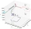 |
Fig. 3 Typical trajectory for a particle, here an electron. Note the Speiser-like oscillatory motion inside the current sheet. Axis scales are given in cell numbers, with 9 cells representing one initial electron inertial length de. Dot colors are the particle Lorentz factor. Solid lines are projections onto the x-y, y-z, and z-x planes. The y direction is not described in the simulations and is here reconstructed on the basis of an invariance of the electromagnetic fields along y. |
3.2. Inflow: two-scale diffusion region and sharp transitions
We now examine the inflow of plasma into the diffusion region. In the literature, for antiparallel reconnection (i.e., no guide field), its width is found to scale with the particles inertial length, a result that we show to also hold for relativistic reconnection in Sect. 3.2.1. The originality of the following results is the formation of a very sharp transition at the entrance of the diffusion regions, which we explore in Sect. 3.2.2.
3.2.1. Width of the diffusion region
The diffusion region is, by definition, the area where impeding mechanisms (which can be collisions, inertia and collective interactions, or finite Larmor effects) prevent the particles from responding in an ideal way to the electric fields induced by magnetic flux variations. The magnetic field and the plasma are then not coupled anymore, the former can freely diffuse, and reconnection can start or be sustained. Defining the diffusion region is thus a matter of finding the area where the non-ideal processes dominate ideal behavior.
Defining unambiguous criteria to identify this region is a complex subject (Ishizawa & Horiuchi 2005; Klimas et al. 2010), especially in the presence of a guide field (Hesse et al. 2002, 2004; Liu et al. 2014) in 3D simulations (Pritchett 2013) or in asymmetric configurations (Zenitani et al. 2011b). In our case, as we show in Sect. 3.2.2, there is a sharp increase in particle density when the inflow plasma reaches the central part, where particles are retained by bouncing motions around the reversing magnetic field. It is associated with a sharp drop in inflow velocity, a rise in temperature, and a violation of the frozen-in relation  . We identify the diffusion region with this area of increased density.
 |
Fig. 4 Cut along x through the X point for four simulations, as indicated in the insets. The times are |
Because of their lighter mass and fastest response, electrons remain frozen to the magnetic field longer than ions. The ion diffusion region is thus larger than the electron one. In all the antiparallel simulations, we find the expected two-scale (ion and electron) diffusion region. It can be seen in Fig. 4, where we present a cut along x through an X point at a given time for different simulations. The width δs of the diffusion region is roughly given by the inertial length ds of the corresponding species, defined with the particle density at the center of the diffusion region, i.e., 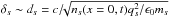 , with throughout all simulations 0.5 ≤ δi/di ≤ 1 and 1 ≤ δe/de ≤ 1.5 (Fig. 5). This is also the scaling found in PIC simulations of non-relativistic ion-electron magnetic reconnection (e.g., Pritchett 2001; Klimas et al. 2010).
In the case of hot background electrons (Tbg,e = 3 × 10⁹ K, with a corresponding background plasma βe = 1.1 × 10⁻²), the transition is less sharp, and the width is larger than the inertial length. The sharpness is discussed in Sect. 3.2.2, and the larger extent is expected because inflowing particles have faster speeds, and thus larger Larmor radii and larger bouncing motions. The width δs should thus also depend on the βs parameter of the inflow.
3.2.2. Sharpness of the inflow boundaries
We see from Fig. 4 that the boundary of the diffusion region, defined by the increase in particle number density, is very sharp in some cases (especially for the case ωce/ωpe = 3 with a cold background plasma). These sharp transitions are not the trace of a shock between the incoming plasma and the over-dense diffusion region. First, because the inflow bulk velocity is not supersonic, in the sense that we have  , with Cfms the phase speed of waves propagating perpendicular to the magnetic field B0, i.e., the fast magnetosonic velocity in MHD (Alfvén and slow waves do not propagate perpendicularly to B0). Second, because the width of the transition between inflow plasma and diffusion region plasma is, in the sharpest case, less than an electron inertial length, while we know that the thermalization of a cold inflow by collisionless kinetic processes occurs on a width of some inertial length, also with the formation of a precursor upstream (e.g., Plotnikov et al. 2013) that is not seen here. Third, because there is no variations in the magnetic field across the sharp particle density variation.
Instead, we explain these sharp transitions by quasi-ballistic motions of the particles entering the diffusion region. Figure 6 shows some particle trajectories: they travel toward the diffusion region because of the electric field E with a guiding center velocity given by vE × B = E × B/B2, then they reach the magnetic field reversal, overshoot to the other side because of their inertia, turn around the increasingly strong magnetic field, and then oscillate around the B = 0 line before being ejected toward the islands (because they have a high vy in the Bx field, see Sect. 3.1 and Fig. 3 for a trajectory in 3D). This explains the fluid point of view of Fig. 4 well: averaging over particles to obtain the fluid particle number density or fluid velocity, the sharpness of the transitions comes from all particles of the same species turning around at roughly the same location.
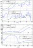 |
Fig. 5 Width of the diffusion region δs, and inertial length ds measured at the center of the diffusion region, for ions and electrons. Panels a) are for the simulation with ωce/ωpe = 3, |
 |
Fig. 6 Trajectories of a sample of particles, and on the right fluid velocities and current for a cut through the X point. |
It also explains the M shape of the particle densities of Fig. 4. Particles spend more time at the edge of the diffusion region, when turning back, than at the center, hence the peaks at the edges and the depletion at the center. The fluid velocity profiles are also well explained by the particle view. We note that an M shape is also reported in the context of the inversion electric field layer (Chen et al. 2011, and references therein). Here we do not find any trace of the inversion layer in the electric field. A possible explanation may be that our electrons are relativistic.
Concerning the sharp transitions, the question is thus to know why and under which conditions all the particles of a species turn back at the same location. They will do so if they all enter the diffusion region with the same velocity, i.e., if their thermal velocity is lower than their bulk velocity:  . Table 3 presents the ratio
  for the different simulations of Fig. 4. For a given magnetization, here ωce/ωpe = 3, we clearly see a correlation between a small and a sharp transition. In particular, in the case with very hot electrons (
 ) and relatively cold ions (
 ), the electron particle number and velocities present smooth variations, while the same curves for ions do exhibit sharp transitions. This is in accordance with the explanation of sharp transitions by the cold nature, in terms of the ratio
  , of the inflowing plasma.
The influence of the magnetization on the sharpness of the transitions is seen by comparing the two first simulations of Table 3, with ωce/ωpe = 1 and 3 and same ratio (plotted in the top part of Fig. 4). A smaller magnetization implies a smoother shape. We understand this as a consequence of particles turning back on a scale given by their Larmor radii in the magnetic field at the sheet entrance, which is smaller when ωce/ωpe is higher.
As a final remark concerning resolution, we note that in the coldest cases, the thermal Larmor radius of the electrons is smaller than a cell length. The resolution of the Larmor radius on the grid is, however, not important for integrating particle trajectories in constant fields, because interpolation of field quantities to particle position then provides the same (constant) values, regardless of the cell size. What matters is the temporal resolution, ωcsΔt < 1 (see Melzani et al. 2013, Sect. 3.1, for a discussion). Here, we have ωcsΔt = 0.04 and 0.12 for ωce/ωpe = 1 or 3. Also, a test run with a spatial and temporal resolution increased by a factor two leads to the same structures.
In summary, the sharp transitions are explained by collective bouncing motions allowed by the cold nature of the inflow:  . Such transitions may also occur in non-relativistic reconnection, but then the inflow speed
  is low and the background plasma should be very cold. They are likely to be more common in relativistic reconnection, where is larger. This may be why, to our knowledge, they have never been reported in other simulations.
Values related to the sharpness of the edge of the diffusion region.
3.3. The relativistic Ohm’s law
We explore the balance of terms in Ohm’s law. The literature concerning 2D non-relativistic reconnection largely shows that for antiparallel reconnection, the dominant term is thermal inertia either in ion-electron (Klimas et al. 2010; Shay et al. 2007; Fujimoto 2009) or pair (Bessho & Bhattacharjee 2005) plasmas, and this is the key element of various analytical models (e.g., Hesse et al. 2011). On the other hand, reconnection with a guide field is sustained by electron bulk inertia on skin-depth scales, and thermal inertia on Larmor radius scales (Hesse et al. 2002, 2004; Liu et al. 2014). Existing studies with relativistic pair plasmas confirm the non-relativistic trend: with no guide field, Hesse & Zenitani (2007), Bessho & Bhattacharjee (2012), and Zenitani et al. (2009a) find a dominating contribution of thermal inertia, while with a guide field Hesse & Zenitani (2007) find a significant contribution of the time derivative of bulk momentum  . Here we explore the situation in ion-electron relativistic plasmas for antiparallel reconnection. We show for the first time in the antiparallel case that bulk inertia contributes at least as much as thermal inertia for high inflow magnetizations. We explain that this is due to a relativistic inflow magnetization in Sect. 3.8.
Ohm’s law is the fluid equation of motion for the lighter particles (the electrons) and is a means to evaluating the relative weight of the different non-ideal terms, allowing reconnection with a simple fluid picture. Understanding the weight and localization of each term is a first step toward building an effective resistivity for fluid models (resistive MHD, two-fluid codes, hybrid codes), where concrete resistive parametrizations can lead to very different behaviors, for instance changing from steady to unsteady states in Zenitani et al. (2009b) or triggering (or not) a Petsheck-like configuration depending on the localization and gradients of the resistivity (Baty et al. 2006).
The relativistic Ohm’s law for electrons is directly derived from the equation of conservation of momentum for the electron fluid, Eq. (B.4), which is itself obtained from Vlasov equation in Appendix B. It reads as 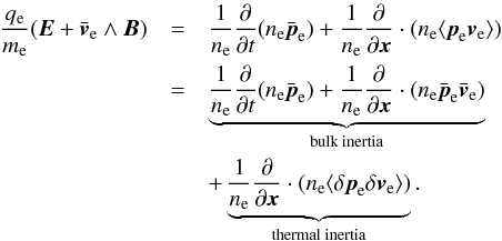 (8)Here we use for simplicity quantities computed in the simulation (or lab) frame; e.g., ne is the electron number density in the labframe (denoted by nlab,e in Appendix B). Brackets ⟨ ·⟩ s or an overbar denote an average in momentum space over the particles distribution function. We also used the definition
  where p = γv is the momentum. The left hand side of Eq. (8) is the ideal part and is set equal to 0 in ideal MHD. On the right hand side are terms linked to finite inertia (i.e., particles do not respond perfectly to the electric field variations because of their inertia):
-
The first term is a part of bulk inertia. However, it vanishes in steady state so we neglect it (validated a posteriori).
-
The second term is inertia linked to the bulk flow and is denoted as bulk inertia. It comes from the overall structure of the flow around the sheet (the profiles of the mean quantities: increase in
 ,
,  ).
). -
The third term is inertia linked to microscopic thermal motion and is denoted as thermal inertia. It comes from the divergence of the off-diagonal terms of the pressure tensor and can be anticipated by a study of the temperature curves.
We analyze Ohm’s law in the direction of the reconnection electric field ( here). Given the invariance along y, the divergence terms have two contributions: ∑ k∂k(pkvy) = ∂x(pxvy) + ∂z(pzvy). A computation of the divergence requires a smoothing of the quantities, especially for the thermal inertia term, which is very noisy.
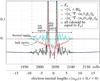 |
Fig. 7 Different components of Ohm’s law (Eq. (8)) for a cut along x through an X point (the same as in Figs. 2, 4 upper right, 8, 9 right, and 10). Run ωce/ωpe = 3, |

We show in Fig. 7 the results for a cut through the X point for the simulation with ωce/ωpe = 3 and Tbg = 1.5 × 10⁷ K ( ). Ohm’s law is satisfied everywhere, except at the sharp transitions at the entrance of the electron diffusion region, where the derivatives diverge. Different areas emerge:
-
The electrons are ideal outside of the ion diffusion region.
-
In the ion diffusion region,
 decreases linearly. The bulk inertia term
  rises linearly to compensate. The term
  wins out over
  . The contribution of the former is understandable when looking at
  and
and  , which increase when we get closer to the sheet in this region (see Fig. 4 for ). The thermal inertia term ∑ k∂k(neδpkδvy) is slightly positive, and partly cancels the contribution of bulk inertia. This cancellation is also reported in Fujimoto (2009) and Klimas et al. (2010) for non-relativistic ion-electron plasmas, and in Bessho & Bhattacharjee (2012) for relativistic pairs. Only ∂x(neδpxδvy) contributes and is negative, which is easily seen when looking at the temperature curves Txy,e and Tzy,e (Fig. 8).
 -
In the electron diffusion region, the
 term vanishes (because B is very weak and
  ). The bulk inertia term is constant and due only to the term , which is expected to contribute, given that
  and
and  in this region (Fig. 9). The other term, , vanishes because
  in this area. The thermal inertia term ∑ k∂k(neδpkδvy) contributes as much as the bulk inertia term. Only ∂x(neδpxδvy) contributes, and it is negative, which is easily seen when looking at the temperature curves Txy,e and Tzy,e in Fig. 8.
A cut along x through other X points in the simulation leads to the same results. Also, a cut along z through the X point reveals that the results of the electron region hold throughout the center of the current sheet, with a slow increase in the term as we get near the islands.
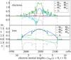 |
Fig. 8 Temperatures for a cut along x through the same X point as in Figs. 2, 4 upper right, 9 right, and 10. Run with ωce/ωpe = 3, |
 |
Fig. 9 Cut along z through the X point. Left: run ωce/ωpe = 1, |

In summary, non-ideal terms in the ion regions are due to bulk inertia and, in the electron diffusion region, to an interestingly equal contribution of bulk and thermal inertia. For other runs with ωce/ωpe = 3 ( to 89), we also find an equal contribution from thermal and bulk inertia. For the most magnetized run, ωce/ωpe = 6 (
 ), the contribution of bulk inertia exceeds that of thermal inertia by a factor 1.5 to 3. We show in Sect. 3.8 with analytical estimations that the high magnetization for electrons indeed allows bulk inertia to overreach thermal inertia, with the former scaling as
  and the latter as
  . This effect is present in our simulations and not in the references previously mentioned with antiparallel fields, because our background electron magnetization is greater. It is thus a new regime that challenges the thermal inertia paradigm at high electron magnetizations. We discuss the possible consequences in Sect. 5.2.
3.4. Outflow: energy content of the exhaust jets
Energy content of the outflows.
It can easily be shown (Sect. 3.4.1) from analytical considerations that the outflows from the diffusion region should have relativistic bulk velocities and/or relativistic temperatures. In our simulation data, the thermal part always clearly dominates the bulk kinetic energy part, and more strongly for more relativistic cases (Sect. 3.4.2). A refined analytical estimate explains why in Sect. 3.8.
3.4.1. A simple analytical estimation
As explained in Sect. 3.1, bipolar outflow jets are naturally produced from each side of the X points. They are clearly visible in Fig. 2. An estimation of the energy content of these outflows can be easily obtained in steady state by using the conservation of particle number and of energy. To do so, we consider that the diffusion region for species s has a length Ds (along z) and a width δs (along x). We generalize the situation to cases where there is a guide field BG. We denote quantities entering (leaving) this region by a subscript “in” (“out”, respectively).
Conservation of particle number (Eq. (B.3)) gives nin,svin,sDs = nout,svout,sδs. Regarding energy conservation (Eq. (B.9)), the inflow energy flux includes the particle energies, and the reconnecting and guide field Poynting fluxes (Eqs. (1) and (2)):  . We assume that in the outflow the energy in the reconnected magnetic field B0 is negligible compared to particle energy, so that the energy flux is
  . Equating the two fluxes and combining this with the conservation of particle number, we obtain
  (9)with
  . The guide field is usually merely compressed, so that 1 − α ≃ 0.
Equation (9) is independent of the p dependence of the distribution function fs. However, some insight can be gained by considering a distribution that is isotropic in the comoving frame, for which we have the result  , with h0 the comoving enthalpy (as defined and pictured for a Maxwell-Jüttner distribution in Fig. B.1), and
  . If, in addition, we neglect the contribution of the guide field and assume an inflow plasma with non-relativistic temperatures and non-relativistic velocities, Eq. (9) becomes 2
 (11)We underline that the magnetization
  is to be taken at the entrance of the diffusion region of species s, where it can differ from its asymptotic value because of a decrease in magnetic field and particle number density (as in Fig. 4).
From Eq. (11), we clearly see that for a relativistic inflow plasma where B2/μ0>nmc2 and hence  , magnetic reconnection is expected to produce outflows with either relativistic bulk velocities (Γout,s> 1) or relativistic temperatures (h0,out,s> 1), or both. We also see that since
  , electrons will be more accelerated/heated than ions and that relativistic electrons (
 ) can be expected even at low ion magnetizations (
 ).
).
3.4.2. Results from simulations
We first check whether the energy estimate of Eqs. (9) and (11) holds in all simulations. This is the case up to a factor ≲ 2. An only approximate correspondence is to be expected because this relation assumes a simple geometry with, in particular, a constant inflow velocity along the diffusion region and no energy exchange between the species. For example, in Fig. 4, for ωce/ωpe = 3 and Tbg = 1.5 × 10⁷ K, we measure  in the inflow for ions and 6.2 for electrons, while at the outflow maximal velocity (Fig. 9) we have
  for ions and 13 for electrons. These orders of magnitude hold for all cases.
A more refined analysis of the energy content of the outflow, split into its thermal and bulk contributions, can be performed. To do so, we decompose the particle energy flux as (see Appendix B) ![Mathematical equation: \begin{equation} \label{equ:particles_energy_flux} \begin{aligned} n_s \langle &\gamma m_s c^2 \vec{v}\rangle_s = n_s m_sc^2 h_{0,\mathrm{out},s} \Gamma_{\mathrm{out},s} \bar{\vec{v}}_{\mathrm{out},s} \\ &= n_s m_sc^2 \bar{\vec{v}}_{\mathrm{out},s} \left[1 + (\Gamma_{\mathrm{out},s}-1) + \Gamma_{\mathrm{out},s}(h_{0,\mathrm{out},s}-1)\right]. \end{aligned} \end{equation}](/articles/aa/full_html/2014/10/aa24083-14/aa24083-14-eq299.png) (12)On the right hand side, the first term is the restmass energy flux and is the same as from the inflow. The second is the kinetic energy of a cold bulk flow of velocity
(12)On the right hand side, the first term is the restmass energy flux and is the same as from the inflow. The second is the kinetic energy of a cold bulk flow of velocity  . The third is the energy transported by thermal motions in the plasma restframe and by pressure work, and we denote it as the enthalpy flux. We note that these definitions match those of Zenitani et al. (2009a), who performed a similar analysis with two-fluid simulations of relativistic reconnection in pair plasmas.
We measure the maximum outflow velocity  , deduce the Lorentz factor Γout,s, measure the maximum in momentum
  , and compute the enthalpy
  . From these values, we estimate in Table 4 the balance of particle energy between each of the terms of Eq. (12).
In all cases, a large fraction of the particle energy flux is in thermal kinetic energy, not in bulk flow kinetic energy. For electrons, we see that the thermal part clearly dominates more as one increases the relativistic nature of the inflow (e.g., 69% in the thermal part for the less relativistic case, 99% for the most relativistic). This is also the case for ions: from 80% to 92% in the thermal part as the ion magnetization increases. The Tbg,i = 2 × 10⁸ K case is exceptional with 91% in the thermal energy, but this high percentage is likely explained by interactions with the hot electrons Tbg,e = 3 × 10⁹ K. We explain why thermally dominated outflows are expected at high inflow magnetization with a refined analytical model in Sect. 3.8.
3.5. Islands structure
Turning to the magnetic islands, we emphasize that they are magnetically isolated, have an M-shaped density distribution, and are hot with anisotropic temperatures. After being expelled along ± z in the outflow, the particles meet the magnetic islands that separate each pair of X points. The islands are initially formed by the tearing of the current sheet. They then consist only of particles of the current sheet, plus those of the background plasma that were inside the current sheet location. Small at the beginning, they grow by collecting particles from the outflows at their periphery and by merging with other islands. A remarkable property is that particles from the background plasma cannot enter the islands, but are scattered by the strong magnetic field structure surrounding the island and circle around it. Consequently, the particles at the island centers remain the same throughout the whole simulation, even after many island-merging events. This matter is explored in more detail in Melzani et al. (2014b). We stress here two main points.
First, the trapped particles are heated by the island contraction (which occurs when two islands merge), so that the central temperatures are very high for both species, highly anisotropic (Figs. 9 and 10), with a dominance of Tzz. The island centers are also where the currents are the strongest.
Second, as said above, most of the inflowing background particles populate a region around the center, while the central part of the island mainly consists of particles originally from the current sheet. As a result, the surrounding part becomes denser than the isolated central part after some time. A cut along z through an island center indeed (Fig. 9) reveals, for the particle density, an M shape with a central dip and two shoulders. This may explain observed density dips at the center of magnetic islands during magnetotail reconnection events (Khotyaintsev et al. 2010), without invoking island merging or particle escape along the flux tube.
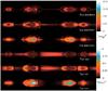 |
Fig. 10 Temperatures for same simulation and time as in Figs. 2, 4 upper right, 8, and 9 right. Note the different units for ions and electrons. Since mic2 = 25mec2, the ions are actually hotter than the electrons. |
3.6. Reconnection electric field and reconnection rate
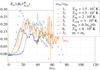 |
Fig. 11 Time evolution of the normalized reconnection electric field |

The rate of variation in magnetic field flux across an X point,  , is equal in 2D configurations to the y component Ey of the electric field at the X-point location. In addition, dΦBz/ dt is in part determined by the outflow velocity, because the latter sets the rate at which magnetic field is extracted from around the X point (see, e.g., in a resistive MHD context, Borovsky & Hesse 2007; Cassak & Shay 2007). Since one expects
  in non-relativistic setups, the reconnection rate Ey is usually normalized either to
  , with
  the hybrid Alfvén speed of Eq. (7), or to
  , with
  the Alfvén speed in the inflow of Eq. (6a). These normalizations are chosen so that the normalized rate, E∗ = Ey/B0VA, stays close to the same set of values. For example, it has been shown that it gives identical results when varying the mass ratio (e.g., Hesse et al. 1999; or Ricci et al. 2002, 2003, for mi/me = 25,180,1836 with an implicit PIC code)3.
In the following we turn to our relativistic case and ask whether a normalization can be found that confines the range of values for E∗ in a narrow range and relaxes to the above normalization in the non-relativistic case. We argue here that the normalization by the hybrid Alfvén speed is not relevant, because it does not depend on the particle number density of the inflow, while the ratio Ey/B0 clearly does. This is seen for the simulation with nbg = 0.3ncs(0), for which Ey/B0 peaks at 0.13c, compared to the otherwise identical simulation with nbg = 0.1ncs(0), where Ey/B0 peaks at 0.20c. On the other hand, the inflow Alfvén speed  , and thus leads to closer normalized rates. We consequently exclude hybrid quantities for normalization.
In a relativistic configuration, the non-relativistic Alfvén speed can increase to infinity. However, the ratio Ey/B0 is also the E × B velocity of the incoming plasma and cannot exceed the speed of light. The normalizing Alfvén velocity should thus also saturate to some value, which is why we choose to normalize the electric field by  (13)with
  the relativistic Alfvén speed in the inflow (Eq. (6b)), which cannot exceed c. The time evolution of E∗ is shown in Fig. 11. Several comments can be made.
First, the rate E∗ is not sensitive to the background plasma temperatures, as can be seen for the simulations ωce/ωpe = 3, nbg = 0.1ncs(0), no guide field, and Tbg = 1.5 × 10⁷, 2 × 10⁸ and 3 × 10⁹ K. This contrasts with the interpretation of Hesse & Zenitani (2007), who attribute a lower rate to a higher inflow temperature. In addition to the temperatures, the magnetization of their simulation also changes and may also affect the rates. Coming back to our simulations, we note that we use very low background plasma β (< 10-2, Table 2) and that a weak plasma β dependence is expected for higher values (e.g., TenBarge et al. 2014, have rates E∗ multiplied by ~ 2 when β passes from 0.01 to 1).
Second, the reconnection rate for the simulation with a higher background particle density (nbg = 0.3ncs(0), E∗ = 0.18) remains lower than its counterpart with nbg = 0.1ncs(0) (E∗ = 0.23). This is in line with the pair plasma simulations of Bessho & Bhattacharjee (2012) who found a similar rate for nbg = 0.1ncs(0) (E∗ = 0.19) and a higher rate for nbg = 0.01ncs(0) (E∗ = 0.36). The reconnection rate thus increases with decreasing background plasma density, which is also coherent with the β dependence mentioned above.
Finally, the normalization leads to very similar values of E∗ for the relativistic cases (ωce/ωpe = 3 or 6), with E∗ = 0.17−0.24, but to a significantly lower rate for the less relativistic case (ωce/ωpe = 1), with E∗ = 0.14. More generally, the values for the relativistic cases are higher than those reported in the literature for undriven, symmetric reconnection with zero guide field in non-relativistic ion-electron plasmas. For the peak values of E∗ (once normalized in the same way as here) we can cite: Birn et al. (2001); Pritchett (2001): 0.09, Fujimoto (2006, 2009): 0.15, Daughton et al. (2006): 0.08, Klimas et al. (2010): 0.07−0.09, and the theoretical work of Hesse et al. (2009a,b) predicting a maximum rate of 0.28. Our results thus suggest higher rates for relativistic reconnection, which is already seen in relativistic simulations of pair plasmas with, e.g., Zenitani & Hoshino (2007) (E∗ = 0.2), Cerutti et al. (2012b) (E∗ = 0.17), or Bessho & Bhattacharjee (2012) (E∗ = 0.19 and 0.36).
In conclusion, the relativistic Alfvén speed of the inflow provides the best normalization for the reconnection electric field, in that it is robust from non-relativistic to relativistic flows. Corresponding rates are in a close range (0.14–0.25), which is higher than the rates found in non-relativistic simulations with the same normalization (0.07–0.15). The rate does not depend on the inflow temperature at low β, but is nevertheless not universal: it decreases with increasing background particle number density. Generalization to the presence of a guide field is discussed in Sect. 4.3.
3.7. Hall field and dispersive waves
We can see in Fig. 4 that inside the ion-diffusion region, but outside of the electron-diffusion region, ions have a low fluid velocity, while electrons still E × B drift toward their diffusion region. This results in a net current roughly given by  , which is the Hall current. This current continues along the magnetic separatrices in the outflow direction, and is at the origin of a quadripolar magnetic field directed along
 . This Hall magnetic field, with the quadripolar structure, is present in our simulations. It has a weak intensity (between 1% and 10% of B0). The charge separation between electrons and ions (Fig. 4) also leads to the creation of a Hall electric field directed along
  in the x < 0 region and
  in the x < 0 region. Both the magnetic and electric Hall fields are absent in a simulation with pairs.
The difference in the dynamical response of ions and electrons also allows the existence of waves with a quadratic dispersion relation, ω ∝ k2, below ion scales (either whistler waves or kinetic Alfvén waves, see Rogers et al. 2001). Observations of the same reconnection rate for any simulation model allowing these waves (PIC, electron-MHD, Hall-MHD, two-fluid with and without electron inertia, hybrid simulations, see Birn et al. 2001; Shay et al. 2007; Rogers et al. 2001), as well as theoretical considerations, have led to the thesis that these waves are essential to allow for fast reconnection rates. However, this view is questioned by a number of simulations that do not support quadratic dispersive waves, but still support fast rates (hybrid simulations with no Hall term, pair plasmas, or strong guide field regime, see Karimabadi et al. 2004; Bessho & Bhattacharjee 2005; Daughton et al. 2006; Daughton & Karimabadi 2007; Liu et al. 2014). It is thus interesting to see whether our simulation data can provide any further insight into the matter.
A prediction of the dispersive wave physics is that the reconnection rate is controlled solely by the ion physics and not by the electrons. According to Daughton et al. (2006), it should be independent of the electron diffusion region length. We could, however, not reproduce their analysis because the electron diffusion zone length is, in our case, limited by the standing islands. It cannot stretch to high values, so we are unable to conclude for or against of the dispersive wave paradigm.
However, we underline that the simulation with mi/me = 1 that we performed features an identical (and even slightly greater, Fig. 11) reconnection rate than simulations with mi/me = 25. It thus points toward a negligible influence of the dispersive waves or to another mechanism that allows fast rates in pair plasmas.
3.8. Simulation-based scaling analysis
The energy content of the outflows and the balance between thermal and bulk inertia in Ohm’s law were explored through the simulations in Sects. 3.3 and 3.4. The aim of the present section is to investigate these points with a simple analytical model in order to gain physical insight into these phenomena and to extrapolate our simulation results to a larger parameter space.
We extend the analytical results of Sect. 3.4.1, where particle number and energy conservation allowed an estimation of the quantity h0,out,sΓout,s (Eqs. (9) or (11)) by now also using the equation of conservation of momentum (Eq. (B.4)).
3.8.1. Thermal versus bulk electron inertia
We first investigate the relative weight of thermal and bulk electron inertia. At the center of the electron diffusion region, we learn from Sect. 3.3 that the reconnection electric field is sustained by electron thermal and bulk inertia, with only the terms ∂x(ne ⟨ δpxδvy ⟩) and  contributing to either one of them, respectively.
-
Concerning thermal inertia, the temperature tensor is defined via Eq. (B.10), so that ⟨ δpxδvy ⟩ = c2Θxy,e/ Γe. We see in Fig. 8 that Θxy,e is linear in the electron diffusion region. It vanishes at the center because there the distribution function fe is symmetric with respect to vx. It is maximal at the diffusion region edge with a value
 . Consequently, we approximate the thermal inertia contribution by
  , where δe is the width of the electron diffusion region.
 -
For the bulk inertia term, we use the fact that
 rises linearly from the center to its maximum value denoted by
  over a distance De/ 2 and that
  has a vanishing derivative at the center (Fig. 9). Consequently, it can be estimated as
  .
.
All in all, from Ohm’s law (Eq. (8)), the electric field at the center of the diffusion region is 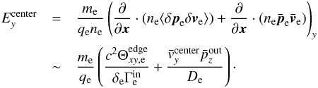 (14)The next step is to use the constancy of Ey, which is respected well in the simulations:
  . We note, however, that at the entrance of the diffusion regions B is different than the asymptotic value B0 and that the E × B drift does not strictly hold (see Fig. 4). If we introduce the inertial length in the inflow,
  , and the inflow magnetization
  , we ultimately obtain
  (15)We now proceed to derive approximate scaling relations for cases where either thermal or bulk inertia dominate the reconnection electric field.
-
First, if thermal inertia dominates over bulk inertia, then Eq. (15) gives
 (16)There are thus several factors contributing to . The diffusion zone width δe is dynamically set during the reconnection process. It can be close to the particles gyroradius at the center of the current sheet or to the plasma inertial length at the center of the current sheet. In all our simulations, we find that the latter assumption holds throughout time to within a factor 2 (Sect. 3.2.1), and in any case,
  is expected to be of order unity. The inflow speed is set by the reconnection electric field,
 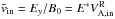 with E∗ the normalized reconnection rate (which lies in the range 0.1−0.25, Sect. 3.6) and the relativistic Alfvén speed in the inflow. For relativistic setups we thus have
  . The inflow magnetization can be arbitrarily large. It is thus the main actor in producing relativistic temperatures, and thermal inertia scales as
  .
. -
Second, the term corresponding to bulk inertia in Eq. (15) can be estimated with the help of Eq. (9) (with
 ,
,  , and neglecting the guide field):
  (17)The ratio δe/De is of order 1 / 10 in our simulations. If we neglect the term
  , which is of order unity for non-relativistic inflow temperatures, we see that bulk inertia scales with .
In conclusion, thermal inertia scales at most as , and bulk inertia as . Consequently, regarding the non-ideal terms in Ohm’s law in the electron diffusion region, we expect bulk inertia to outweight thermal inertia at high inflow electron magnetization.
3.8.2. Energy content of the outflows
We now turn to the energy content of the outflows to see whether we can explain their thermally dominated character for relativistic runs. The temperature in the outflows is dominated by Θxx,e or Θyy,e, which we denote by  . We first have to link to . The outflow temperature at the center of the diffusion region is roughly constant along z throughout the area of linear increase of
  (Fig. 9), because particles on their way from the X point to the exhaust mainly turn into the reconnected magnetic field and thus do not really gain thermal agitation, but convert it from one component of Θ to another. We can thus assume
  . We now would like to assume
  . This indeed holds for electrons in the case of Fig. 8. However, this does not hold in all simulations, and is between 1 / 10 to 10 times
  . This is due to the different origin of these components: reflects particles in Speiser orbits going up and down along x with a zero bulk x velocity, while reflects the asymmetry of the distribution function with respect to vx due to the newly entering particles at the edge of the diffusion zone.
With the previous remark in mind, we still make the hypothesis  . Next, if we assume that thermal inertia contributes significantly in Ohm’s law, we obtain, with the scaling of Eq. (16),
 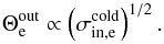 (18)For relativistic temperatures we have
  (Fig. B.1), so that with Eq. (18) we see that a relativistic inflow magnetization implies
  . On the other hand, energy conservation gives, in its simplest form (Eq. (11) with
  ):
): 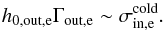 (19)Thus,
  (20)We finally turn to the ratio of energy fluxes in the outflow. We see with Eq. (12) that the flux associated with kinetic bulk energy is Γout,e − 1. With Eq. (20) (and for Γout,e ≫ 1), this flux is
  . The flux associated with thermal kinetic energy and pressure work is h0,out,eΓout,e − 1, and with Eq. (19) we have
 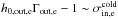 . The ratio of thermal-to-bulk energy fluxes is thus
  , meaning that relativistic inflow magnetization inevitably implies reconnection exhausts dominated by thermal energy, which is what we see in our simulations (Table 4), even if the scalings derived here do not hold exactly because of the many assumptions involved.
In conclusion, we have shown that under the hypothesis of non-ideal effects sustained by thermal inertia, relativistic inflow magnetizations produce thermally dominated outflows. The physical reason is that the reconnection electric field Ey is large in the inflow region, so that thermal inertia must be high in order to sustain Ey in the central region, which implies high temperatures.
However, we also demonstrated that thermal inertia is not expected to dominate for very relativistic inflows. When this is the case, there is no constraints from Ohm’s law on the temperature, and we cannot decide on the ratio of thermal to bulk energy fluxes. Since this ratio is (h0,out,eΓout,e − 1) / (Γout,e − 1) ~ h0,out,e, a relativistic outflow temperature on the order of mec2 suffices to give thermally dominated outflows.
For our simulations, thermal inertia contributes equally or less than bulk inertia (Sect. 3.3), but still significantly, so that the outflows are thermally dominated.
4. Effects of a guide field
Except in special configurations, the generic reconnection geometry involves asymptotic fields that are not antiparallel. An angle different from 180° can be described by the addition of a uniform guide magnetic field to the antiparallel configuration. Such configurations have been largely studied in the non-relativistic case (e.g., Pritchett & Coroniti 2004; Drake et al. 2005; Goldman et al. 2011; Le et al. 2013; Graf von der Pahlen & Tsiklauri 2014), and feature significant differences with the antiparallel case. Here we only focus on the reconnection rates and on the island structure, and postpone a study of other points to a future publication. We present results from two simulations, with BG = 0.5B0 and BG = B0.
4.1. Overall structure
 |
Fig. 12 Top: simulation with |


We first stress that because of the presence of the guide field, in both cases BG = 0.5B0 and B0, the relation B>E holds everywhere through time and space, hence also the relation B>Eperp (with Eperp the component perpendicular to B). Consequently, particle acceleration is not possible in directions perpendicular to B and is only allowed along the field lines at places where E·B ≠ 0. Such parallel electric fields are allowed by the non-idealness of the plasma response,  , and are indeed found at and around the X points.
Just as in the zero guide field case, the plasma accelerated by Ey is slowly deviated by the reconnected Bx component, which produces outflows directed along ± z. However, particles from these outflows feel the Lorentz force from the guide field, and their trajectories are tilted against the z axis, as is evident in Fig. 12. Reversing the guide field from  to tilts them in the opposite direction. We underline that while the tilt angle is indeed smaller for a smaller guide field, it also depends on the background plasma pressure, as shown by TenBarge et al. (2014).
In the present case,  . Electrons are thus accelerated along the field lines in the direction. Their motion along the field lines results in a projected (x-z plane) motion directed toward positive z where
  (i.e., in the x> 0 area), or toward negative z where
  (i.e., in the x < 0 area). It results in large and fast electron flows above and below the current sheet, and to a rotation around the islands in a direction opposed to cyclotron gyration. Ions are accelerated toward and counterstream with respect to the electrons.
Particles reaching the central part are accelerated along y by Ey and, because they always feel a magnetic field B>E, they are guided by the magnetic field and spend more time in the acceleration region for strong BG (Fig. 13). Consequently, is greater than with no guide field under similar conditions, and reaches high values on a larger area (compare in Figs. 2 and 12).
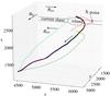 |
Fig. 13 Typical trajectory for a particle, here an electron, for simulation with |
4.2. Islands’ structure
The structure of the islands resembles the no guide field case: their centers are composed of particles initially in the current sheet, with background particles only circling at the periphery. They are the hottest and strongest current-carrying part of the simulations. There are, however, important differences.
First, the inclination of the outflows makes the island asymmetric, with electrons rotating around in a direction opposite to that of ions (when looking at the motion projection in the x-z plane). Second, as islands form and contract, the guide magnetic field is compressed and increases in strength. In the simulation with BG = 0.5B0, it passes from 0.5B0 initially to 1.8−2.1B0 in the islands, while in the simulation with BG = B0, it passes from B0 initially to 2.1−2.4B0 in the islands. Third, because of the strong magnetic field along y, temperatures are isotropized along x and z. (In the no guide field case we had Θzz ~ 2Θxx.) Here Θzz ≃ Θyy ≃ Θxx, equal to up to 4 for electrons and 0.2 for ions. This is a value close to the average (Θzz + Θyy + Θxx) / 3 of the zero guide field case. Off-diagonal terms are an order of magnitude smaller.
4.3. Reconnection electric field and reconnection rate
In the normalization of Sect. 3.6,  , the Alfvén velocity includes the total magnetic field
  ). In the presence of a guide field (α ≠ 0), Alfvén waves propagating along the magnetic field do so in a direction that makes an angle θ = arctanα with the outflow direction . As we explained in Sect. 3.6, the reconnection electric field is in part set by the velocity at which the field lines are extracted from the X point, i.e., by the outflow velocity. This outflow velocity is mostly set by the projection of the Alfvén speed onto the outflow direction (Eq. (10) in the non-relativistic limit, Eq. (9) in the general case). Consequently, it seems justified to normalize the electric field with the projection of the Alfvén speed onto the direction, i.e., to use
 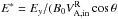 ).
).
Figure 14 shows the time evolution of E∗ for three simulations with BG/B0 = 0, 0.5, 1, with otherwise identical parameters. The peak reconnection rate decreases when the guide field increases: 0.24, 0.22, and 0.20. This is also the kind of dependence found in PIC simulations of ion-electron, non-relativistic reconnection (Ricci et al. 2003; Huba 2005; TenBarge et al. 2014; Liu et al. 2014), relativistic pair reconnection (Hesse & Zenitani 2007), or two-fluid simulations of relativistic reconnection (Zenitani et al. 2009a)4. Consequently, relativistic reconnection in ion-electron plasmas does not bring new effects in this respect. However, we underline that the normalization used here allows minimizing the scatter in E∗ for the various simulations.
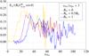 |
Fig. 14 Time evolution of the normalized reconnection electric field |


5. Summary and discussion
5.1. Summary
We investigate magnetic reconnection in low β ion-electron plasmas (mass ratio of 25) with 2D PIC simulations, under relativistic conditions, i.e., the magnetic energy of the inflowing plasma exceeds its restmass energy. The simulations start from a Harris kinetic equilibrium with no localized perturbation. For diagnostics and analytical models, we use momentum and energy fluid equations based on lab-frame quantities (Appendix B). They have the advantage of being valid regardless of the particle distribution function, while the usual relativistic fluid equations using comoving quantities are restricted to isotropic comoving distribution functions.
For antiparallel reconnection, the structure of the diffusion region has a width (in the inflow direction) δs given by the respective inertial length ds of the species s, measured at the center of the diffusion region. A high inflow temperature increases this width. At the entrance of the diffusion regions for simulations at low background β ≤ 2.5 × 10⁻³, we find sharp transitions in the fluid quantities that were not reported elsewhere. We argue that they are not shocks. Instead, they occur when the inflowing particles have a thermal velocity that is far lower than their bulk E × B velocity, so that they enter the diffusion region with the same velocity and bounce back at the same location. We stress that these sharp transitions are not a feature of relativistic reconnection, because they depend only on the cold nature of the inflow. However, the phenomenon should be more common in relativistic reconnection because then the inflow bulk velocity vE × B ~ E/B is large.
We detail the balance of terms in the relativistic Ohm’s law for antiparallel reconnection. The ion diffusion region is dominated by bulk inertia (as defined in Eq. (8)). In the electron diffusion region, bulk inertia contributes equally or more than thermal inertia. The latter result challenges the thermal-inertia-dominated paradigm that holds for non-relativistic or mildly relativistic antiparallel reconnection. We show analytically that a significant contribution of bulk inertia is to be expected whenever the inflow magnetization  (cold, meaning that the temperature is not taken into account, see Eq. (4)) of the electrons is high, because then bulk inertia
 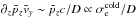 can exceed thermal inertia
  . This is a new result that should hold for any large electron magnetization.
For the reconnection outflows we analytically show from mass and energy conservation that reconnection is expected to produce relativistic outflow temperatures and/or relativistic outflow bulk velocities. From simulations we find that outflow thermal energy dominates over bulk kinetic energy (from 70% to 99%, for simulations with increasing background magnetization). A more refined analytical analysis shows that this is expected if the reconnection electric field is sustained by thermal inertia. If bulk inertia dominates the thermal inertia, as expected at very high inflow magnetization, then our simple analytical model does not allow a conclusion about the cold or hot nature of the outflows. Also, our simulations do not probe high enough electron magnetizations to reach this regime: at  , thermal inertia contributes 50% of the reconnection electric field, and this fraction goes down to 25−40% at
  , which is significant enough for the hypothesis of Erec sustained by thermal inertia to hold.
For the islands we show that, with or without a guide field, their centers consist mainly of particles initially in the current sheet that were gathered inside the island during the tearing instability, that do not mix with the background plasma even after many island merging events. Particles of the background plasma cannot reach the inner parts because of the strong magnetic field surrounding the islands, and thus circle around the central part. As a result, the central part is less dense than its immediate surrounding. This may explain observed density dips at the center of magnetic islands during magnetotail reconnection events (Khotyaintsev et al. 2010), without invoking island merging or particle escape along the flux tube. Islands are also the hottest parts of the flow, with fully anisotropic temperatures in the antiparallel case, and distributions close to gyrotropic with a guide field.
We argue that the reconnection rates are to be normalized by the asymptotic magnetic field and relativistic Alfvén speed in the inflow, projected onto the outflow direction if there is a guide field:  . This leads to rates in a narrow range: E∗ peaks between 0.14–0.25. However, we stress that there is no universal value for E∗ as defined here or elsewhere. First, because other studies show that it depends on the inflow plasma β (increasing with decreasing β). Here we find no dependence on the background plasma temperature, but smaller rates for larger particle number densities. Second, we find larger rates for the relativistic setups (0.18−0.25) than for the mildly relativistic case (0.15). These rates are also larger than those reported in the literature for ion-electron non-relativistic reconnection (0.07−0.15 for Birn et al. 2001; Pritchett 2001; Fujimoto 2006, 2009; Daughton et al. 2006; Klimas et al. 2010). This points toward relativistic reconnection being slightly faster than non-relativistic reconnection. This trend is reinforced by simulations in relativistic pair plasmas (E∗ = 0.3 in our case or, e.g., 0.17−0.36 for Zenitani & Hoshino 2007; Bessho & Bhattacharjee 2012; Cerutti et al. 2012b). We note that this is against the interpretation of Hesse & Zenitani (2007) of a smaller rate for more relativistic setups. Third, we confirm that a guide field leads to a smaller normalized rate.
We explore the consequences of adding a guide magnetic field. The flow structure is strongly disturbed for two reasons: the Lorentz force associated with the guide field, and the relation E < B everywhere. The acceleration region is now defined by the condition E·B ≠ 0. Inflowing ion and electron Larmor radii are smaller than the island scales or magnetic gradient scales, and remain so even after the acceleration phase by Erec, because this phase conserves the perpendicular-to-B momentum. Particles thus remain tied to the field lines everywhere, including in the acceleration region where they spend more time before being deviated in the outflows.
5.2. Discussion and astrophysical outlook
This study may serve as microphysics input for analyses on larger scales concerning magnetic energy conversion in relativistic ion-electron plasmas, as should be encountered in the coronae of AGN and microquasar accretion flows, in the lobe of radio galaxies or inside relativistic jets from AGNs or GRBs. We now discuss such applications and give estimates for key parameters in these objects: magnetic field B, electron number density ne, magnetizations  (where cold means that only the rest mass energy is taken into account, Eq. (4)), with s = i, e for ions or electrons, and Alfvén speeds
  . The properties of magnetic reconnection as studied here only depend on the inflow magnetization and temperatures, regardless of the real values of B and ne. This is true at least as long as effects such as pair creation and annihilation, radiative braking, or Compton drag on the electrons, can be neglected (see Melzani et al. 2014b, for a discussion on these effects).
5.2.1. Toward a new regime: non-dissipative reconnection?
Our finding of a reconnection electric field sustained equally or more by bulk inertia than by thermal inertia for large inflow electron magnetization ( ), and the extrapolation of Sect. 3.8, indicate that bulk inertia might end up dominating at even higher inflow electron magnetizations. This was also envisioned by Hesse & Zenitani (2007), and reconnection in such a regime would bear significant differences with the standard picture. However, we nuance the assertion of Hesse & Zenitani (2007) that reconnection would then be a reversible process: as underlined in Sect. 3.8, the reconnection outflows may be thermally dominated even when bulk inertia dominates Ohm’s law. A definite answer to these questions requires very high magnetizations, which we can hardly reach with a PIC code and which may require relativistic gyrokinetic codes.
Highly magnetized environments, such as pulsar winds near the termination shock ( , Bucciantini et al. 2011; Sironi & Spitkovsky 2011), or other objects with
  discussed in what follows, are likely to support this reconnection regime. We note that magnetar magnetospheres, even if they feature magnetizations exceeding (Lyutikov & Lazarian 2013), support a very different reconnection regime due to pair and photon creations (Uzdensky 2011).
5.2.2. Large scale transient outflow production, the example of microquasars
We have shown that the reconnection outflows are thermally dominated, with a bulk Lorentz factor not necessarily increasing with the inflow magnetization and featuring low values (1.63 at most, Table 4). However, applications to large scale outflows triggered by reconnection events require some care. The outflows studied in the present manuscript originate in the electron diffusion region, and feature ion/electron decoupling. At larger distances, if not bounded by the islands and by our periodic setup, electrons and ions are expected to couple and to follow the ideal MHD dynamic. The scale on which they can propagate is fixed by larger scales than simulated here.
On the other hand, it is expected and observed (Khotyaintsev et al. 2006) that magnetic energy conversion also takes place along the magnetic separatrices far away from the dissipation region, on length scales of hundreds of ion inertial lengths. This conversion occurs through instabilities that produce thermal and non-thermal electrons (Drake et al. 2005; Egedal et al. 2009, 2012), and through the complex structure of collisionless nonlinear waves (slow shock, compound wave, rotational wave) by which the magnetized inflowing plasma transits to the hot and unmagnetized outflow on MHD scales (Liu et al. 2012; Higashimori & Hoshino 2012). It is this large-scale outflow that should be identified as the transient reconnection-driven jets in microquasar models (de Gouveia dal Pino & Lazarian 2005; de Gouveia Dal Pino et al. 2010; Kowal et al. 2011; McKinney et al. 2012; Dexter et al. 2014). In the magnetosphere close to the black hole, de Gouveia dal Pino & Lazarian (2005) estimate on the basis of an analytical model, ne ~ 5 × 1015 cm-3, B ~ 7 × 10⁷ G, which gives electron and ion magnetizations  and
and  , and an Alfvén speed
  . This is clearly in the relativistic regime. The energy content of the large scale outflows in this case has not been studied, but we can expect from the collisionless slow shocks or rotational discontinuities at the separatrices, to produce a thermally dominated outflow. It may not be so for other jet production mechanisms, and could help distinguishing in favor or against reconnection scenarios.
Another unknown is what becomes of the ambient plasma that is expelled by the first reconnected field lines ahead of the dipolarization front. In our study, it would correspond to half of a magnetic island, ejected out of the simulation box. The ambient plasma would be the plasma from the current sheet trapped in the island. As we demonstrate, this plasma does not mix with the reconnected plasma and is simply compressed and heated (see Vapirev et al. 2013, for a 3D case where instabilities imply magnetic to kinetic energy conversion). In an open configuration, it would be at the head of the large scale outflow.
5.2.3. Plasma heating in AGN and microquasar coronae and in galaxy radio lobes
Photon emission in the hard state of microquasars and AGNs is believed to come from inverse-Compton scattering of seed photons by the electrons of a corona. To achieve this, these electrons must reach temperatures on the order of 109 K, i.e., Θe = Te/mec2 ~ 0.2. A non-thermal population of electrons is also required by the observation of MeV photons (Poutanen & Veledina 2014). A proposed mechanism for plasma heating is by magnetic reconnection (Di Matteo 1998; Merloni & Fabian 2001; Reis & Miller 2013). The plasma Alfvén speed estimated by these authors lies in the range 0.03c–0.3c. Associated electron magnetizations are  , which is in the range of the present study. A crucial question is the energy distribution between ions and electrons: if most of the magnetic energy goes to ions, and because of the low collisionality of these dilute environments, a large temperature difference can be sustained (Di Matteo et al. 1997). Our study shows that ions are slightly more heated than electrons. This can be seen with the temperatures of Figs. 8–10, and 12. More generally, the kinetic energy of the particles trapped in the magnetic islands is distributed as 55% for ions and 45% for electrons, and the kinetic energy of the particles from the background plasma that are accelerated when reaching the current sheet is also distributed as 60% for ions and 40% for electrons (for details see Melzani et al. 2014b). The energy distribution by acceleration processes far downstream of the diffusion region requires another study.
Similar questions arise concerning the heating of the lobes of radio galaxies (Kronberg et al. 2004). There, n ~ 3 × 10⁻⁶ cm-3 for the number densities, and B ~ 5 μG for the equipartition magnetic field with values that can be locally ten times higher, which gives magnetizations  and Alfvén speeds ~ 0.02c − 0.2c. Our conclusion for the energy repartition between ions and electrons also holds.
5.2.4. Flares and “mini”-jets in extragalactic jets and in GRBs
Flare-like activity in the GeV–TeV range is observed from extragalactic jets and may possibly be explained by local reconnection events inside the jet, which produce smaller jets (the reconnection exhausts) which in turn radiate the expected photons (Giannios et al. 2009). This γ-ray emission region may be located close to the black hole ( < 0.05 pc, Giroletti et al. 2004), where B ~ 0.02−0.2 G and the plasma magnetization is high. For example, Giannios et al. (2009) take  , which leads to
  and VA ~ c. This is in the regime where bulk inertia should dominate in Ohm’s law. Also, Giannios et al. (2009) use energy considerations to estimate that the blobs emitted from the reconnection exhausts should be ~ 1014 cm, i.e., based on its estimated particle density, 1010 ion inertial lengths. Here again, the physics far from the dissipation region should play an important role in producing such large scale structures.
5.2.5. Radio emission from extragalactic jets
Another case for relativistic magnetic reconnection is inside jets from AGNs on scales of 10−100 kpc. Radio spectra may be explained by radiation linked to reconnection events (Romanova & Lovelace 1992). Observations of AGN jets indicate B ~ 10−30 μG, n ~ 0.8−5 × 10⁻⁸ cm-3, and electron magnetizations in the range  (Schwartz et al. 2006), which implies ion magnetizations
  and Alfvén speeds ~ 0.5−0.8c. Again, our results apply in these cases, and in particular the electron magnetizations are in the very relativistic range where bulk inertia should dominate in Ohm’s law.
5.2.6. High-energy particle production
The proposed normalization of the reconnection rate,  ) with the relativistic inflow Alfvén speed, leads to E∗ in a close range (0.14−0.25), and because it only relies on inflow quantities, it allows for an easy prediction of the reconnection electric field. In particular, the ratio Erec/B0 is a key quantity for estimating the time scale of energy dissipation or the maximum energy gain for particles. It is interesting to notice that for very relativistic plasmas, saturates at c, so that Erec/B0 saturates at ~ 0.2c. It may imply that the hardness of the high-energy tails saturates. We explore these matters in a forthcoming paper (Melzani et al. 2014b). Briefly, we find for a given species a power-law tail whenever its background magnetization is relativistic (above a few), with an index depending mainly on the inflow magnetization.
5.2.7. Other complications
We finally point out that the present study is oversimplified in many respects. Magnetic reconnection in magnetized coronae and jets probably often implies asymmetric plasmas from each side of the current sheet, guide fields (Aunai et al. 2013; Hesse et al. 2013; Eastwood et al. 2013), and also normal fields (along  here) reminiscent of the ambient magnetic field. The last point has been studied in the context of the Earth magnetotail (Pritchett 2005a, 2010; Sitnov & Swisdak 2011). Also, the initial conditions chosen in the simulations are arbitrary and do not necessarily reflect the real environments. Explored alternatives to the Harris sheet include X-point collapse (e.g., Graf von der Pahlen & Tsiklauri 2014) or force-free equilibrium (e.g., Liu et al. 2014) and show little differences with the Harris case. However, 3D initial configurations should also be considered, because in a real environment most of the energy dissipation may occur at 3D nulls, involving for example spine-fan reconnection, or at quasi-separatrix layers (Birn & Priest 2007; Pontin 2011). Few kinetic simulations exist for such setups (Baumann & Nordlund 2012; Olshevsky et al. 2013). A related point is the external forcing, i.e., the large scale plasma flow that can increase the magnetic field gradients and trigger reconnection. Studies (Pei et al. 2001; Pritchett 2005b; Ohtani & Horiuchi 2009; Klimas et al. 2010) show that the reconnection rate E∗ is then fixed by the boundary conditions, and is thus larger than the spontaneous rate. The timescale of the forcing also proves to be important (Pei et al. 2001). These considerations, as well as some of the points made earlier on, highlight the multiscale nature of reconnection in the context of concrete astrophysical objects – and demonstrate the need for corresponding multiscale simulation studies, a field still in its infancy (e.g., Horiuchi et al. 2010; Innocenti et al. 2013)
Another central question is the validity of the 2D findings in three dimensions. Magnetic islands then become extended filaments, modulated or broken by instabilities in the third dimension or by a lack of coherence of the tearing instability (Daughton et al. 2011; Kagan et al. 2013; Markidis et al. 2013). It may imply more mixing of the current sheet particles with those of the background plasma. Concerning the validity of our claims on Ohm’s law, 3D PIC simulations in non-relativistic plasmas have shown that anomalous resistivity due to microinstabilities remains a negligible dissipation mechanism in the diffusion region (Liu et al. 2013; Karimabadi et al. 2013), where the reconnection electric field is still sustained by thermal electron inertia. The scaling analysis of Sect. 3.8 should thus remain valid, as should the conclusion that bulk inertia dominates at high inflow magnetization.
Throughout this section, “all the results” means the time evolution of the reconnection rate and of the width of the diffusion zone for electrons and ions, the distribution functions of high-energy particles, the temperature curves in the diffusion zone, the energy content in the outflows, as well as the relative weight of the terms in Ohm’s law.
We note that the non-relativistic limit of Eq. (11), with h0,out,s ~ 1 and  , is
, is
 (10)
where
(10)
where  is the non-relativistic inflow Alfvén speed with only the mass of species s. It only comprises the component B0, so that if there is a guide field, this is the projection of the total Alfvén speed onto the outflow direction .
However, going down to mi/me = 1 leads to less systematic results. For example, Fujimoto (2009) reports E∗ = 0.15 for mi/me = 100 and 0.08 for pairs. Liu et al. (2014) report close rates for mi/me = 1 and 25. Here we performed a simulation with mi/me = 1 and find a peak reconnection rate E∗ = 0.30, which is greater than for mi/me = 25 (Fig. 11).
We note, however, that in asymmetric reconnection the rate increases with the guide field strength, see Aunai et al. (2013), Hesse et al. (2013).
Acknowledgments
We thank the referee, D. Uzdensky, for comments that allowed to significantly improve the manuscript. M. Melzani would like to thank H. Baty, B. Cerutti, and M. E. Innocenti for stimulating discussions. The simulations were performed using HPC resources from GENCI (Grand Équipement National de Calcul Intensif) at CINES, CCRT, and IDRIS under the allocation x2013046960. Tests were conducted at pôle scientifique de modélisation numérique, PSMN, at the École Normale Supérieure de Lyon, whose staff we thank for their steady technical support. This work has been financially supported by the Programme National Hautes Energies (PNHE).
References
- Aunai, N., Hesse, M., Zenitani, S., et al. 2013, Phys. Plasmas, 20, 022902 [NASA ADS] [CrossRef] [Google Scholar]
- Barkov, M., Komissarov, S. S., Korolev, V., & Zankovich, A. 2014, MNRAS, 438, 704 [NASA ADS] [CrossRef] [Google Scholar]
- Baty, H., Priest, E. R., & Forbes, T. G. 2006, Phys. Plasmas, 13, 022312 [NASA ADS] [CrossRef] [Google Scholar]
- Baty, H., Petri, J., & Zenitani, S. 2013, MNRAS, 436, L20 [NASA ADS] [CrossRef] [Google Scholar]
- Baumann, G., & Nordlund, Å. 2012, ApJ, 759, L9 [NASA ADS] [CrossRef] [Google Scholar]
- Bessho, N., & Bhattacharjee, A. 2005, Phys. Rev. Lett., 95, 245001 [NASA ADS] [CrossRef] [Google Scholar]
- Bessho, N., & Bhattacharjee, A. 2012, ApJ, 750, 129 [NASA ADS] [CrossRef] [Google Scholar]
- Birk, G. T., Crusius-Wätzel, A. R., & Lesch, H. 2001, ApJ, 559, 96 [NASA ADS] [CrossRef] [Google Scholar]
- Birn, J., Drake, J. F., Shay, M. A., et al. 2001, J. Geophys. Res., 106, 3715 [Google Scholar]
- Birn, J., & Priest, E. R. 2007, Reconnection of magnetic fields : magnetohydrodynamics and collisionless theory and observations (Cambridge University Press) [Google Scholar]
- Biskamp, D. 2000, Magnetic Reconnection in Plasmas, ed. D. Biskamp, (Cambridge University Press) [Google Scholar]
- Blackman, E. G., & Field, G. B. 1994, Phys. Rev. Lett., 72, 494 [NASA ADS] [CrossRef] [Google Scholar]
- Borovsky, J. E., & Hesse, M. 2007, Phys. Plasmas, 14, 102309 [NASA ADS] [CrossRef] [Google Scholar]
- Bucciantini, N., Arons, J., & Amato, E. 2011, MNRAS, 410, 381 [Google Scholar]
- Bulanov, S. V., & Sasorov, P. V. 1976, Sov. Astron., 19, 464 [Google Scholar]
- Cassak, P. A., & Shay, M. A. 2007, Phys. Plasmas, 14, 102114 [NASA ADS] [CrossRef] [Google Scholar]
- Cerutti, B., Uzdensky, D. A., & Begelman, M. C. 2012a, ApJ, 746, 148 [Google Scholar]
- Cerutti, B., Werner, G. R., Uzdensky, D. A., & Begelman, M. C. 2012b, ApJ, 754, L33 [NASA ADS] [CrossRef] [Google Scholar]
- Cerutti, B., Werner, G. R., Uzdensky, D. A., & Begelman, M. C. 2013, ApJ, 770, 147 [NASA ADS] [CrossRef] [Google Scholar]
- Cerutti, B., Werner, G. R., Uzdensky, D. A., & Begelman, M. C. 2014, ApJ, 782, 104 [NASA ADS] [CrossRef] [Google Scholar]
- Chen, L.-J., Daughton, W. S., Lefebvre, B., & Torbert, R. B. 2011, Phys. Plasmas, 18, 012904 [NASA ADS] [CrossRef] [Google Scholar]
- Coppi, B., Laval, G., & Pellat, R. 1966, Phys. Rev. Lett., 16, 1207 [NASA ADS] [CrossRef] [Google Scholar]
- Daughton, W., & Karimabadi, H. 2007, Phys. Plasmas, 14, 072303 [NASA ADS] [CrossRef] [Google Scholar]
- Daughton, W., Scudder, J., & Karimabadi, H. 2006, Phys. Plasmas, 13, 072101 [NASA ADS] [CrossRef] [Google Scholar]
- Daughton, W., Roytershteyn, V., Karimabadi, H., et al. 2011, Nature Phys., 7, 539 [Google Scholar]
- de Gouveia dal Pino, E. M., & Lazarian, A. 2005, A&A, 441, 845 [NASA ADS] [CrossRef] [EDP Sciences] [Google Scholar]
- de Gouveia Dal Pino, E. M., Piovezan, P. P., & Kadowaki, L. H. S. 2010, A&A, 518, A5 [NASA ADS] [CrossRef] [EDP Sciences] [Google Scholar]
- Dexter, J., McKinney, J. C., Markoff, S., & Tchekhovskoy, A. 2014, MNRAS, 440, 2185 [NASA ADS] [CrossRef] [Google Scholar]
- Di Matteo, T. 1998, MNRAS, 299, L15 [NASA ADS] [CrossRef] [Google Scholar]
- Di Matteo, T., Blackman, E. G., & Fabian, A. C. 1997, MNRAS, 291, L23 [NASA ADS] [CrossRef] [Google Scholar]
- Drake, J. F., Shay, M. A., Thongthai, W., & Swisdak, M. 2005, Phys. Rev. Lett., 94, 095001 [NASA ADS] [CrossRef] [PubMed] [Google Scholar]
- Drenkhahn, G., & Spruit, H. C. 2002, A&A, 391, 1141 [NASA ADS] [CrossRef] [EDP Sciences] [Google Scholar]
- Dungey, J. W. 1958, in Electromagnetic Phenomena in Cosmical Physics, ed. B. Lehnert, IAU Symp., 6, 135 [Google Scholar]
- Eastwood, J. P., Phan, T. D., Øieroset, M., et al. 2013, Plasma Phys. Control. Fusion, 55, 124001 [NASA ADS] [CrossRef] [Google Scholar]
- Egedal, J., Daughton, W., Drake, J. F., Katz, N., & Lê, A. 2009, Phys. Plasmas, 16, 050701 [NASA ADS] [CrossRef] [Google Scholar]
- Egedal, J., Daughton, W., & Le, A. 2012, Nature Phys., 8, 321 [Google Scholar]
- Fujimoto, K. 2006, Phys. Plasmas, 13, 072904 [NASA ADS] [CrossRef] [Google Scholar]
- Fujimoto, K. 2009, Phys. Plasmas, 16, 042103 [NASA ADS] [CrossRef] [Google Scholar]
- Gedalin, M. 1993, Phys. Rev. E, 47, 4354 [NASA ADS] [CrossRef] [Google Scholar]
- Giannios, D., Uzdensky, D. A., & Begelman, M. C. 2009, MNRAS, 395, L29 [NASA ADS] [CrossRef] [Google Scholar]
- Giovanelli, R. G. 1947, MNRAS, 107, 338 [NASA ADS] [CrossRef] [Google Scholar]
- Giovanelli, R. G. 1948, MNRAS, 108, 163 [NASA ADS] [CrossRef] [Google Scholar]
- Giroletti, M., Giovannini, G., Feretti, L., et al. 2004, ApJ, 600, 127 [NASA ADS] [CrossRef] [Google Scholar]
- Goldman, M. V., Lapenta, G., Newman, D. L., Markidis, S., & Che, H. 2011, Phys. Rev. Lett., 107, 135001 [NASA ADS] [CrossRef] [Google Scholar]
- Goodman, J., & Uzdensky, D. 2008, ApJ, 688, 555 [NASA ADS] [CrossRef] [Google Scholar]
- Graf von der Pahlen, J., & Tsiklauri, D. 2014, Phys. Plasmas, 21, 012901 [Google Scholar]
- Hesse, M., & Zenitani, S. 2007, Phys. Plasmas, 14, 112102 [Google Scholar]
- Hesse, M., Schindler, K., Birn, J., & Kuznetsova, M. 1999, Phys. Plasmas, 6, 1781 [Google Scholar]
- Hesse, M., Kuznetsova, M., & Hoshino, M. 2002, Geophys. Res. Lett., 29, 1563 [NASA ADS] [CrossRef] [Google Scholar]
- Hesse, M., Kuznetsova, M., & Birn, J. 2004, Phys. Plasmas, 11, 5387 [Google Scholar]
- Hesse, M., Zenitani, S., Kuznetsova, M., & Klimas, A. 2009a, Phys. Plasmas, 16, 102106 [NASA ADS] [CrossRef] [Google Scholar]
- Hesse, M., Zenitani, S., Kuznetsova, M., & Klimas, A. 2009b, Phys. Plasmas, 16, 129906 [NASA ADS] [CrossRef] [Google Scholar]
- Hesse, M., Neukirch, T., Schindler, K., Kuznetsova, M., & Zenitani, S. 2011, Space Sci. Rev., 160, 3 [NASA ADS] [CrossRef] [Google Scholar]
- Hesse, M., Aunai, N., Zenitani, S., Kuznetsova, M., & Birn, J. 2013, Phys. Plasmas, 20, 061210 [NASA ADS] [CrossRef] [Google Scholar]
- Higashimori, K., & Hoshino, M. 2012, J. Geophys. Res., 117, 1220 [Google Scholar]
- Horiuchi, R., Usami, S., Ohtani, H., & Moritaka, T. 2010, Plasma Fusion Res., 5, 2006 [NASA ADS] [CrossRef] [Google Scholar]
- Huba, J. D. 2005, Phys. Plasmas, 12, 012322 [NASA ADS] [CrossRef] [Google Scholar]
- Innocenti, M. E., Lapenta, G., Markidis, S., Beck, A., & Vapirev, A. 2013, J. Comput. Phys., 238, 115 [NASA ADS] [CrossRef] [Google Scholar]
- Ishizawa, A., & Horiuchi, R. 2005, Phys. Rev. Lett., 95, 045003 [NASA ADS] [CrossRef] [Google Scholar]
- Jaroschek, C. H., Hoshino, M., Lesch, H., & Treumann, R. A. 2008, Adv. Space Res., 41, 481 [NASA ADS] [CrossRef] [Google Scholar]
- Ji, H., & Daughton, W. 2011, Phys. Plasmas, 18, 111207 [NASA ADS] [CrossRef] [Google Scholar]
- Kagan, D., Milosavljević, M., & Spitkovsky, A. 2013, ApJ, 774, 41 [NASA ADS] [CrossRef] [Google Scholar]
- Karimabadi, H., Krauss-Varban, D., Huba, J. D., & Vu, H. X. 2004, J. Geophys. Res., 109, 9205 [CrossRef] [Google Scholar]
- Karimabadi, H., Roytershteyn, V., Daughton, W., & Liu, Y.-H. 2013, Space Sci. Rev., 178, 307 [NASA ADS] [CrossRef] [Google Scholar]
- Khotyaintsev, Y. V., Vaivads, A., Retinò, A., et al. 2006, Phys. Rev. Lett., 97, 205003 [NASA ADS] [CrossRef] [Google Scholar]
- Khotyaintsev, Y. V., Vaivads, A., André, M., et al. 2010, Phys. Rev. Lett., 105, 165002 [NASA ADS] [CrossRef] [Google Scholar]
- Kirk, J. G., & Skjæraasen, O. 2003, ApJ, 591, 366 [NASA ADS] [CrossRef] [Google Scholar]
- Klimas, A., Hesse, M., Zenitani, S., & Kuznetsova, M. 2010, Phys. Plasmas, 17, 112904 [NASA ADS] [CrossRef] [Google Scholar]
- Koide, S., & Arai, K. 2008, ApJ, 682, 1124 [NASA ADS] [CrossRef] [Google Scholar]
- Kojima, Y., Oogi, J., & Kato, Y. E. 2011, A&A, 531, A47 [NASA ADS] [CrossRef] [EDP Sciences] [Google Scholar]
- Kowal, G., de Gouveia Dal Pino, E. M., & Lazarian, A. 2011, ApJ, 735, 102 [NASA ADS] [CrossRef] [Google Scholar]
- Kronberg, P. P., Colgate, S. A., Li, H., & Dufton, Q. W. 2004, ApJ, 604, L77 [NASA ADS] [CrossRef] [Google Scholar]
- Lapenta, G., & Lazarian, A. 2012, Nonlinear Processes Geophys., 19, 251 [NASA ADS] [CrossRef] [Google Scholar]
- Larrabee, D. A., Lovelace, R. V. E., & Romanova, M. M. 2003, ApJ, 586, 72 [Google Scholar]
- Lazar, A., Nakar, E., & Piran, T. 2009, ApJ, 695, L10 [NASA ADS] [CrossRef] [Google Scholar]
- Lazarian, A., & Vishniac, E. T. 1999, ApJ, 517, 700 [NASA ADS] [CrossRef] [Google Scholar]
- Lazarian, A., Eyink, G. L., & Vishniac, E. T. 2012, Phys. Plasmas, 19, 012105 [NASA ADS] [CrossRef] [Google Scholar]
- Le, A., Egedal, J., Ohia, O., et al. 2013, Phys. Rev. Lett., 110, 135004 [NASA ADS] [CrossRef] [Google Scholar]
- Liu, Y.-H., Drake, J. F., & Swisdak, M. 2012, Phys. Plasmas, 19, 022110 [NASA ADS] [CrossRef] [Google Scholar]
- Liu, Y.-H., Daughton, W., Karimabadi, H., Li, H., & Roytershteyn, V. 2013, Phys. Rev. Lett., 110, 265004 [NASA ADS] [CrossRef] [Google Scholar]
- Liu, Y.-H., Daughton, W., Karimabadi, H., Li, H., & Peter Gary, S. 2014, Phys. Plasmas, 21, 022113 [NASA ADS] [CrossRef] [Google Scholar]
- Loureiro, N. F., Schekochihin, A. A., & Cowley, S. C. 2007, Phys. Plasmas, 14, 100703 [NASA ADS] [CrossRef] [Google Scholar]
- Loureiro, N. F., Samtaney, R., Schekochihin, A. A., & Uzdensky, D. A. 2012, Phys. Plasmas, 19, 042303 [NASA ADS] [CrossRef] [Google Scholar]
- Lyubarsky, Y. E. 2005, MNRAS, 358, 113 [NASA ADS] [CrossRef] [Google Scholar]
- Lyutikov, M. 2006a, MNRAS, 369, L5 [NASA ADS] [CrossRef] [Google Scholar]
- Lyutikov, M. 2006b, MNRAS, 367, 1594 [CrossRef] [Google Scholar]
- Lyutikov, M., & Lazarian, A. 2013, Space Sci. Rev., 178, 459 [NASA ADS] [CrossRef] [Google Scholar]
- Lyutikov, M., & Uzdensky, D. 2003, ApJ, 589, 893 [NASA ADS] [CrossRef] [Google Scholar]
- Markidis, S., Henri, P., Lapenta, G., et al. 2013, Phys. Plasmas, 20, 082105 [NASA ADS] [CrossRef] [Google Scholar]
- McKinney, J. C., & Uzdensky, D. A. 2012, MNRAS, 419, 573 [Google Scholar]
- McKinney, J. C., Tchekhovskoy, A., & Blandford, R. D. 2012, MNRAS, 423, 3083 [NASA ADS] [CrossRef] [Google Scholar]
- Melzani, M., Walder, R., Folini, D., & Winisdoerffer, C. 2014a, Int. J. Mod. Phys. Conf. Ser., 28, 60194 [CrossRef] [Google Scholar]
- Melzani, M., Walder, R., Folini, D., Winisdoerffer, C., & Favre, J. M. 2014b, A&A, 570, A112 [NASA ADS] [CrossRef] [EDP Sciences] [Google Scholar]
- Melzani, M., Winisdoerffer, C., Walder, R., et al. 2013, A&A, 558, A133 [NASA ADS] [CrossRef] [EDP Sciences] [Google Scholar]
- Merloni, A., & Fabian, A. C. 2001, MNRAS, 321, 549 [NASA ADS] [CrossRef] [Google Scholar]
- Mihalas, D., & Mihalas, B. W. 1984, Foundations of radiation hydrodynamics, eds. D. Mihalas, & B. W. Mihalas (New York: Oxford University Press) [Google Scholar]
- Ohtani, H., & Horiuchi, R. 2009, Plasma and Fusion Research, 4, 24 [NASA ADS] [CrossRef] [Google Scholar]
- Olshevsky, V., Lapenta, G., & Markidis, S. 2013, Phys. Rev. Lett., 111, 045002 [NASA ADS] [CrossRef] [Google Scholar]
- Paschmann, G., Øieroset, M., & Phan, T. 2013, Space Sci. Rev., 178, 385 [NASA ADS] [CrossRef] [Google Scholar]
- Pei, W., Horiuchi, R., & Sato, T. 2001, Phys. Plasmas, 8, 3251 [NASA ADS] [CrossRef] [Google Scholar]
- Pétri, J., & Kirk, J. G. 2007, Plasma Phys. Control. Fusion, 49, 1885 [NASA ADS] [CrossRef] [Google Scholar]
- Pétri, J., & Lyubarsky, Y. 2007, A&A, 473, 683 [NASA ADS] [CrossRef] [EDP Sciences] [Google Scholar]
- Plotnikov, I., Pelletier, G., & Lemoine, M. 2013, MNRAS, 430, 1280 [NASA ADS] [CrossRef] [Google Scholar]
- Pontin, D. I. 2011, Adv. Space Res., 47, 1508 [NASA ADS] [CrossRef] [Google Scholar]
- Poutanen, J., & Veledina, A. 2014, Space Sci. Rev., 1 [Google Scholar]
- Priest, E. R. 1987, Solar magneto-hydrodynamics. (Dordrecht: D. Reidel) [Google Scholar]
- Pritchett, P. L. 2001, J. Geophys. Res., 106, 3783 [Google Scholar]
- Pritchett, P. L. 2005a, J. Geophys. Res., 110, 5209 [CrossRef] [Google Scholar]
- Pritchett, P. L. 2005b, J. Geophys. Res., 110, 10213 [CrossRef] [Google Scholar]
- Pritchett, P. L. 2010, J. Geophys. Res., 115, 10208 [CrossRef] [Google Scholar]
- Pritchett, P. L. 2013, Phys. Plasmas, 20, 061204 [NASA ADS] [CrossRef] [Google Scholar]
- Pritchett, P. L., & Coroniti, F. V. 2004, J. Geophys. Res., 109, 1220 [Google Scholar]
- Reis, R. C., & Miller, J. M. 2013, ApJ, 769, L7 [Google Scholar]
- Ricci, P., Lapenta, G., & Brackbill, J. U. 2002, Geophys. Res. Lett., 29, 3 [Google Scholar]
- Ricci, P., Lapenta, G., & Brackbill, J. U. 2003, Phys. Plasmas, 10, 3554 [NASA ADS] [CrossRef] [Google Scholar]
- Rogers, B. N., Denton, R. E., Drake, J. F., & Shay, M. A. 2001, Phys. Rev. Lett., 87, 195004 [NASA ADS] [CrossRef] [Google Scholar]
- Romanova, M. M., & Lovelace, R. V. E. 1992, A&A, 262, 26 [NASA ADS] [Google Scholar]
- Sakai, J.-I., Saito, S., Mae, H., et al. 2002, Phys. Plasmas, 9, 2959 [NASA ADS] [CrossRef] [Google Scholar]
- Schwartz, D. A., Marshall, H. L., Lovell, J. E. J., et al. 2006, ApJ, 640, 592 [NASA ADS] [CrossRef] [Google Scholar]
- Shay, M. A., Drake, J. F., & Swisdak, M. 2007, Phys. Rev. Lett., 99, 155002 [NASA ADS] [CrossRef] [Google Scholar]
- Sironi, L., & Spitkovsky, A. 2011, ApJ, 741, 39 [NASA ADS] [CrossRef] [Google Scholar]
- Sironi, L., & Spitkovsky, A. 2014, ApJ, 783, L21 [NASA ADS] [CrossRef] [Google Scholar]
- Sitnov, M. I., & Swisdak, M. 2011, J. Geophys. Res., 116, 12216 [CrossRef] [Google Scholar]
- Takahashi, H. R., Kudoh, T., Masada, Y., & Matsumoto, J. 2011, ApJ, 739, L53 [NASA ADS] [CrossRef] [Google Scholar]
- Takamoto, M. 2013, ApJ, 775, 50 [NASA ADS] [CrossRef] [Google Scholar]
- Tenbarge, J. M., Hazeltine, R. D., & Mahajan, S. M. 2010, MNRAS, 403, 335 [NASA ADS] [CrossRef] [Google Scholar]
- Tenbarge, J. M., Daughton, W., Karimabadi, H., Howes, G. G., & Dorland, W. 2014, Phys. Plasmas, 21, 020708 [NASA ADS] [CrossRef] [Google Scholar]
- Treumann, R. A., & Baumjohann, W. 2013, Front. Phys., 1 [Google Scholar]
- Uzdensky, D. A. 2006 [arXiv:astro-ph/0607656] [Google Scholar]
- Uzdensky, D. A. 2011, Space Sci. Rev., 160, 45 [NASA ADS] [CrossRef] [Google Scholar]
- Uzdensky, D. A., Loureiro, N. F., & Schekochihin, A. A. 2010, Phys. Rev. Lett., 105, 235002 [NASA ADS] [CrossRef] [Google Scholar]
- Vapirev, A. E., Lapenta, G., Divin, A., et al. 2013, J. Geophys. Res., 118, 1435 [CrossRef] [Google Scholar]
- Watanabe, N., & Yokoyama, T. 2006, ApJ, 647, L123 [NASA ADS] [CrossRef] [Google Scholar]
- Zanotti, O., & Dumbser, M. 2011, MNRAS, 418, 1004 [NASA ADS] [CrossRef] [Google Scholar]
- Zenitani, S., & Hesse, M. 2008, ApJ, 684, 1477 [NASA ADS] [CrossRef] [Google Scholar]
- Zenitani, S., & Hoshino, M. 2001, ApJ, 562, L63 [NASA ADS] [CrossRef] [Google Scholar]
- Zenitani, S., & Hoshino, M. 2005a, ApJ, 618, L111 [NASA ADS] [CrossRef] [Google Scholar]
- Zenitani, S., & Hoshino, M. 2005b, Phys. Rev. Lett., 95, 095001 [NASA ADS] [CrossRef] [PubMed] [Google Scholar]
- Zenitani, S., & Hoshino, M. 2007, ApJ, 670, 702 [NASA ADS] [CrossRef] [Google Scholar]
- Zenitani, S., & Hoshino, M. 2008, ApJ, 677, 530 [NASA ADS] [CrossRef] [Google Scholar]
- Zenitani, S., Hesse, M., & Klimas, A. 2009a, ApJ, 705, 907 [NASA ADS] [CrossRef] [Google Scholar]
- Zenitani, S., Hesse, M., & Klimas, A. 2009b, ApJ, 696, 1385 [NASA ADS] [CrossRef] [Google Scholar]
- Zenitani, S., Hesse, M., & Klimas, A. 2011a, in AIP Conf. Ser. 1366, eds., V. Florinski, J. Heerikhuisen, G. P. Zank, & D. L. Gallagher, 138 [Google Scholar]
- Zenitani, S., Hesse, M., Klimas, A., & Kuznetsova, M. 2011b, Phys. Rev. Lett., 106, 195003 [NASA ADS] [CrossRef] [Google Scholar]
Appendix A: Relativistic Harris equilibrium
We derived the equilibrium relations for relativistic temperatures and current drift speeds, as well as for arbitrary ion to electron mass ratio and temperature ratio, in Melzani et al. (2013).
Each species follows a Maxwell-Jüttner distribution:  (A.1)with s = i for ions or e for electrons, μs = 1 / Θs = msc2/Ts,
  , and K2 the modified Bessel function of the second kind. We note that fs is indeed normalized with respect to
  to ncs(x) (Melzani et al. 2013), so that the particle density in the simulation frame is ncs(x), and that in the comoving plasma frame of each species is n0,cs(x) = ncs(x) / Γs. Loading the distribution A.1 when both Θs and Us are relativistic is non-trivial, and we use the method explained in Melzani et al. (2013).
For the special case where ions and electrons have the same temperatures, fulfilling Vlasov and Maxwell’s equations leads to 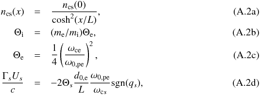 with sgn(qs) the sign of the charge qs, ωcs = eB0/ms the cyclotron pulsation defined in the asymptotic magnetic field B0 (e> 0 here),
 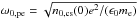 the electron plasma pulsation defined by the comoving number density n0,cs(0) = ncs(0) / Γs at the center of the current sheet, and d0,e = c/ω0,pe the associated inertial length.
Inserting Eqs. (A.2c) into (A.2d), the latter becomes 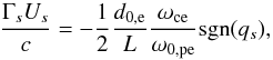 (A.3)so that we see that Eqs. (A.2a)−(A.2c) and (A.3) are well suited to expressing the equilibrium relations in terms of the comoving quantities ωce/ω0,pe and L/d0,e alone. Some manipulations are needed to express everything in terms of the lab-frame quantities ωce/ωpe and L/de, where ωpe is the counterpart of ω0,pe in the simulation frame (
 ), and de = c/ωpe. To do so, we note in Eq. (A.2d) that ω0,ped0,e = c = ωpede, and we express Eq. (A.2c) as Θe = Γe(ωce/ωpe)2/ 4. With this, we obtain
 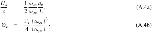 We see from Eq. (A.4a) that we have the condition ωce/ωpe < 2L/de. If this is not the case, the equilibrium cannot be achieved. Why it is so can be seen by rewriting Eq. (A.2d) as Θe = (L/ 2de)(ωce/ωpe)ΓeUe/c: satisfying Vlasov equation is possible only if Θe < (L/ 2de)(ωce/ωpe)Γe, but this is not possible if the pressure balance condition (which is Eq. (A.4b)) requires a temperature exceeding this limit to balance the magnetic field pressure.
As a final note, we express the thermal Larmor radius of the particles, defined as ⟨ (γvperp)2 ⟩ 1 / 2/ωce where ⟨·⟩ is an average over the distribution function, at current sheet center: 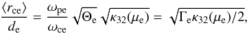 (A.5)where the first part of the equality is general (Melzani et al. 2013), and the second is obtained for the Harris equilibrium using Eq. (A.4b) for the ratio ωce/ωpe. The function κ32 is the plasma comoving enthalpy and is plotted in Fig. B.1. The thermal Larmor radius is consequently temperature dependent via κ32(1 / Θe).
Appendix B: From Vlasov to fluid equations
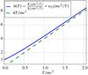 |
Fig. B.1 Normalized comoving enthalpy for species s: h0s = (n0s ⟨ γmsc2 ⟩ s + Ps) / (n0smsc2), for a Maxwell-Jüttner distribution of temperature Ts. For the background plasma temperatures considered in this study, T = (1.5 × 10⁷, 2 × 10⁸, 3 × 10⁹) K, we have for electrons Θe = (2.5 × 10⁻³, 3.4 × 10⁻², 0.51) and corresponding h0e = (1.006, 1.086, 2.57), while h0i ~ 1 always holds for ions. |
Appendix B.1: Fluid equations
Fluid equations employed in numerical codes are usually expressed in terms of comoving quantities, such as, for species s, the comoving particle number density n0s, the comoving enthalpy h0s, the comoving pressure P0s, and in terms of the fluid velocity  and its associated Lorentz factor Γs. The conservation of particle number and of momentum for each species, and of total energy, then read as (see e.g., Mihalas & Mihalas 1984; Barkov et al. 2014)
 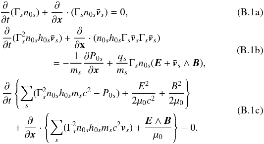 These equations are, however, not well suited to analysis of particle simulations. First, because accessible quantities are those defined in the simulation (or lab) frame, while those in the comoving frame of the plasma must be obtained by a boost at the local mean speed . Second, because they assume a comoving particle distribution that is isotropic in momentum space in order to use a scalar pressure P0s instead of the full pressure tensor and, as we show below, to write relations such as
 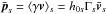 for the mean momentum. This is not the case in the out-of-equilibrium plasmas that we study.
Instead, we derive the fluid equations directly from the collisionless Vlasov equation. The latter reads as 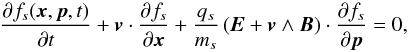 (B.2)where p = γv, and fs is the distribution function in the simulation or lab frame. We denote its counterpart in the comoving frame by f0s.
The first moment (with 1) of Eq. (B.2) gives the equation of conservation of the number of particles:  (B.3)We note that nlab,s = Γsn0s, so that we indeed recover Eq. (B.1).
The second moment (with p) gives the equation of conservation of momentum:  (B.4)We used the definition
  , where p = γv is the momentum, and similarly for δv. Also, ⟨ ·⟩ s denotes an average in p over the distribution function fs. To recover Eq. (B.1a), we use the relation
  for the mean momentum, which is only valid if the comoving distribution f0s is isotropic in p (Melzani et al. 2013). Also, we note that the stress tensor is defined as
  , and is also equal (again if f0s is isotropic) to
 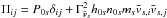 . Inserting these expressions into Eq. (B.4) does lead to Eq. (B.1a). We also note that Eq. (B.4) can be put into a conservative form by using the conservation of momentum for the electromagnetic field, which reads as
 ![Mathematical equation: \appendix \setcounter{section}{2} \begin{equation} \label{equ:field_momentum} \frac{\partial}{\partial t}\epsilon_0(\vec{E}\wedge \vec{B}) - \frac{\partial}{\partial \vec{x}}\cdot \vec{T} = -[\rho \vec{E} + \textbf{j}\wedge \vec{B}], \end{equation}](/articles/aa/full_html/2014/10/aa24083-14/aa24083-14-eq541.png) (B.5)where
(B.5)where  is Maxwell stress tensor, ρ = ∑ sqsnlab,s is the charge density, and
  is the current density. One thus has to sum Eq. (B.4) over all species and then use Eq. (B.5), to obtain
 ![Mathematical equation: \appendix \setcounter{section}{2} \begin{eqnarray} \label{equ:fluid_2_cons} \ \frac{\partial}{\partial t} \left(\epsilon_0 \vec{E}\wedge \vec{B} + \sum_sm_sn_{\mathrm{lab},s}\bar{\vec{p}}_s\right) + \frac{\partial}{\partial \vec{x}}\cdot \left(-\textbf{T} + \sum_sm_sn_{\mathrm{lab},s}\left[\bar{\vec{p}}_s\bar{\vec{v}}_s +\langle \delta \vec{p}_s\delta \vec{v}_s\rangle_s\right]\right) = 0. \end{eqnarray}](/articles/aa/full_html/2014/10/aa24083-14/aa24083-14-eq545.png) (B.6)Finally, multiplying Vlasov Eq. (B.2) by γmsc2 and integrating over p gives the equation of conservation of energy:
(B.6)Finally, multiplying Vlasov Eq. (B.2) by γmsc2 and integrating over p gives the equation of conservation of energy: 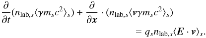 (B.7)The righthand side accounts for the coupling between the species and the electromagnetic fields, and thus possibly with other species via collective interactions. The non-relativistic limit of this equation is easily obtained by making the difference between Eqs. (B.7) and (B.3). Also, Eq. (B.7) can be put into a useful conservative form by expressing its righthand side through the energy equation for the fields, which is
 ![Mathematical equation: \appendix \setcounter{section}{2} \begin{equation} \begin{aligned} \frac{\partial}{\partial t} & \left(\frac{E^2}{2\mu_0c^2}+\frac{B^2}{2\mu_0}\right)+\frac{\partial}{\partial \vec{x}}\cdot \frac{\vec{E}\wedge \vec{B}}{\mu_0} = -\vec{E}\cdot \vec{j} \\[1.5mm] & = -\textbf{E} \cdot \sum_s \int\mathrm{d}^3 \vec{p}f_s (\vec{x}, \vec{p})q_s \vec{v} \\[1.5mm] & = - \sum_s n_\mathrm{lab,s} q_s \langle \vec{v}\cdot \vec{E}\rangle_s. \end{aligned} \end{equation}](/articles/aa/full_html/2014/10/aa24083-14/aa24083-14-eq548.png) (B.8)We thus have to sum Eq. (B.7) for all species, to obtain
(B.8)We thus have to sum Eq. (B.7) for all species, to obtain 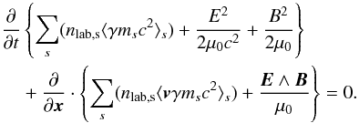 (B.9)To recover Eq. (B.1b), we use the relation
  (Melzani et al. 2013, Table 5), and the relations previously used for
  and nlab,s.
Appendix B.2: Measure of the temperature tensor
The kinetic temperature is a second-order moment of the particle distribution function and is, as such, not always suited to characterizing the velocity distribution of a population strongly out-of-equilibrium. We nevertheless use it as an indication of the thermal energy content of the population, and of the momentum flux transfers, the latter being especially relevant to Ohm’s law. We define the temperature tensor as the ratio of the pressure tensor nlab,sms ⟨ δpsδvs ⟩ s (appearing in the equation of conservation of momentum, Eq. (B.4)), to the comoving particle number density n0s. Since nlab,s = Γsn0,s, the temperature tensor is 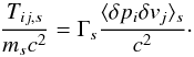 (B.10)For the special case of a Maxwell-Jüttner distribution function of temperature Θs = 1 /μs = Ts/ (msc2), of drift velocity β0,s and associated Lorentz factor Γ0,s, given in the simulation frame by
 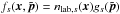 ,
,  , and
, and 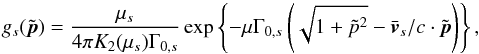 (B.11)we do have (Melzani et al. 2013) ⟨ δpiδvj ⟩ s/c2 = Θsδij/ Γs where δij is Kronecker’s delta. We also note that this distribution is normalized to unity:
  . Based upon these considerations, we measure the temperatures with expression (B.10).
All Tables
Physical input parameters of the simulations and resulting magnetizations of the background plasma.
All Figures
|
Fig. 1 Electron number density in the whole simulation domain, at two different times. From run ωce/ωpe = 3, |
| In the text | |
|
Fig. 2 Zoom around a X point showing various fluid quantities. From run ωce/ωpe = 3, |
| In the text | |
|
Fig. 3 Typical trajectory for a particle, here an electron. Note the Speiser-like oscillatory motion inside the current sheet. Axis scales are given in cell numbers, with 9 cells representing one initial electron inertial length de. Dot colors are the particle Lorentz factor. Solid lines are projections onto the x-y, y-z, and z-x planes. The y direction is not described in the simulations and is here reconstructed on the basis of an invariance of the electromagnetic fields along y. |
| In the text | |
|
Fig. 4 Cut along x through the X point for four simulations, as indicated in the insets. The times are |
| In the text | |
|
Fig. 5 Width of the diffusion region δs, and inertial length ds measured at the center of the diffusion region, for ions and electrons. Panels a) are for the simulation with ωce/ωpe = 3, |
| In the text | |
|
Fig. 6 Trajectories of a sample of particles, and on the right fluid velocities and current for a cut through the X point. |
| In the text | |
|
Fig. 7 Different components of Ohm’s law (Eq. (8)) for a cut along x through an X point (the same as in Figs. 2, 4 upper right, 8, 9 right, and 10). Run ωce/ωpe = 3, |
| In the text | |
|
Fig. 8 Temperatures for a cut along x through the same X point as in Figs. 2, 4 upper right, 9 right, and 10. Run with ωce/ωpe = 3, |
| In the text | |
|
Fig. 9 Cut along z through the X point. Left: run ωce/ωpe = 1, |
| In the text | |
|
Fig. 10 Temperatures for same simulation and time as in Figs. 2, 4 upper right, 8, and 9 right. Note the different units for ions and electrons. Since mic2 = 25mec2, the ions are actually hotter than the electrons. |
| In the text | |
|
Fig. 11 Time evolution of the normalized reconnection electric field |
| In the text | |
|
Fig. 12 Top: simulation with |
| In the text | |
|
Fig. 13 Typical trajectory for a particle, here an electron, for simulation with |
| In the text | |
|
Fig. 14 Time evolution of the normalized reconnection electric field |
| In the text | |
|
Fig. B.1 Normalized comoving enthalpy for species s: h0s = (n0s ⟨ γmsc2 ⟩ s + Ps) / (n0smsc2), for a Maxwell-Jüttner distribution of temperature Ts. For the background plasma temperatures considered in this study, T = (1.5 × 10⁷, 2 × 10⁸, 3 × 10⁹) K, we have for electrons Θe = (2.5 × 10⁻³, 3.4 × 10⁻², 0.51) and corresponding h0e = (1.006, 1.086, 2.57), while h0i ~ 1 always holds for ions. |
| In the text | |
Current usage metrics show cumulative count of Article Views (full-text article views including HTML views, PDF and ePub downloads, according to the available data) and Abstracts Views on Vision4Press platform.
Data correspond to usage on the plateform after 2015. The current usage metrics is available 48-96 hours after online publication and is updated daily on week days.
Initial download of the metrics may take a while.