| Issue |
A&A
Volume 531, July 2011
|
|
|---|---|---|
| Article Number | A47 | |
| Number of page(s) | 5 | |
| Section | Astrophysical processes | |
| DOI | https://doi.org/10.1051/0004-6361/201116562 | |
| Published online | 09 June 2011 | |
Relativistic magnetic reconnection at X-type neutral points
Department of PhysicsHiroshima University, Higashi-Hiroshima 739-8526, Japan
e-mail: This email address is being protected from spambots. You need JavaScript enabled to view it.
Received: 24 January 2011
Accepted: 1 April 2011
Abstract
Context. The relativistic effects in the oscillatory damping of magnetic disturbances near two-dimensional X-points are investigated.
Aims. By taking displacement current into account, we study new features of extremely magnetized systems, in which the Alfvén velocity is almost the speed of light.
Methods. The frequencies of the least-damped mode are calculated using linearized relativistic MHD equations for wide ranges of the Lundquist number S and the magnetization parameter σ.
Results. The oscillation and decay times depend logarithmically on S in the low resistive limit. This logarithmic scaling is the same as for nonrelativistic dynamics, but the coefficient becomes small as ~σ − 1/2 with increasing σ. These timescales approach constant values in the high resistive limit: the oscillation time becomes a few times the light crossing time, irrespective of σ, and the decay time is proportional to σ so is longer for a highly magnetized system.
Key words: magnetohydrodynamics (MHD) / magnetic reconnection / relativistic processes
© ESO, 2011
1. Introduction
The importance of magnetic reconnection manifests itself in various energetic astrophysical phenomena, including relativistic objects such as pulsars, magnetars, active galactic nuclei, and gamma ray bursts. The characteristic propagation velocity for magnetic disturbances, the Alfvén velocity, depends on the magnetization parameter σ: 2σ represents the ratio of the magnetic to the rest-mass energy density of the plasma. When the magnetization parameter σ ≫ 1, the Alfvén velocity is almost the speed of light; the velocity becomes nonrelativistic in the opposite limit, σ ≪ 1. In this paper, we consider some inherently relativistic features that may appear in the magnetic reconnection when σ is large.
In a simple analysis of the Sweet-Parker type reconnection, the structure of the reconnection layer depends on two large dimensionless numbers: σ and the Lundquist (or magnetic Reynolds) number S, an inverse of resistivity (Lyutikov & Uzdensky 2003). For σ ≪ S, the inflow velocity is nonrelativistic, and the reconnection is very similar to the classical Sweet-Parker model. However, for σ ≫ S ≫ 1, the inflow velocity becomes relativistic. Lyubarsky (2005) incorporated the compressibility of matter and found that the inflow velocity is always sub-Alfvénic and remains much less than the speed of light, contradicting Lyutikov & Uzdensky (2003). The reconnection rate is still estimated by substituting c for the Alfvén velocity in the nonrelativistic formula, even in the relativistic regime.
Small differences may also come from assuming a steady state. Numerical simulations of an anti-parallel magnetic configuration in two dimensions have been performed without assuming a steady state using relativistic resistive MHD code (Watanabe & Yokoyama 2006), a relativistic two-fluid model (Zenitani et al. 2009), and PIC simulations on a kinetic scale (Zenitani & Hoshino 2005, 2007, 2008). See also Komissarov (2007) for the numerical schemes of the resistive relativistic MHD. These approaches have clearly demonstrated the relativistic dynamics, but simulation in a wide range of parameters would be time-consuming. Moreover, the resolution becomes poor for low resistivity.
The dynamics at an X-type null point, where a current sheet forms and the magnetic energy is dissipated, have been already studied. In the context of nonrelativistic dynamics, Craig & McClymont (1991) considered the behavior of MHD waves near the X-point in the cold plasma approximation using linear perturbation theory. They show the remarkable result that the dissipation time behaves as ~ (lnS)2. This logarithmic dependence, in contrast to the normal power behavior ~Sα, indicates fast decay. Subsequently, the problem was studied analytically (Hassam 1992) and by considering the propagation of linearized waves (McLaughlin & Hood 2004). Some physical properties of a more realistic system have also been included, such as nonlinear waves with thermal pressure (McClymont & Craig 1996; McLaughlin et al. 2009), electron inertial effects (McClements et al. 2004), and viscosity (Craig et al. 2005; Craig 2008). See a recent review of this topic by McLaughlin et al. (2010) and the references therein.
The main concern of this paper is to explore the relativistic effects on the dynamical reconnection at an X-point. In particular we consider whether the reconnection is qualitatively modified for a highly magnetized system with σ ≫ 1, such as a magnetar. We adopt a very simple system in order to understand the differences, if any. Our work is a relativistic extension of Craig & McClymont (1991); that is, we calculate complex normal frequencies, which determine the oscillatory damping of the magnetic disturbances with small amplitudes, neglecting thermal pressure, viscosity, and so on. The problem may be solved as an initial value problem, but the initial data inevitably contain electromagnetic waves besides MHD waves, and subsequent evolution may be complex. In Sect. 2, we discuss our numerical methods and boundary conditions. Our results are shown in Sect. 3. Section 4 contains our conclusions.
2. Model
2.1. Equations for relativistic dynamics
We consider a two-dimensional problem, assuming ∂/∂z = 0. In our model, the magnetic field B is located on a plane and the electric field is perpendicular to it, E = Eez. The electric current jez is also perpendicular to the plane, and the charge density consistently vanishes, since ∇·E = 0. These electromagnetic fields can be expressed in terms of only the z-component of a vector potential A = Aez as  (1)The flux function A satisfies with a wave equation with a source term:
  (2)where the displacement current is included in contrast to the usual nonrelativistic treatment.
The dynamics of the plasma flow is determined by the continuity equation  (3)and the momentum equation with the Lorentz force
  (4)where γ = (1 − (v/c)2) − 1/2, ρ is the mass number density in the laboratory frame, and the proper one is ρ/γ. In Eq. (4), the Coulomb force vanishes and thermal effects in the pressure and internal energy are neglected in the cold limit. This cold plasma approximation simplifies the problem. The slow magnetoacoustic wave is absent. In nonrelativistic dynamics, it is found that propagation of the fast one causes the current density to accumulate at the X point, where the energy is dissipated (McLaughlin & Hood 2004; McLaughlin et al. 2009). Thermal pressure is neglected, since our concern is the propagation in linearized system. The finite pressure is meaningful in fully nonlinear dynamics, where coupling and mode conversion between MHD waves are important in the neighborhood of the dissipation zone.
Ohm’s law with resistivity η can be written as  (5)which, in terms of A, is
  (6)The relativistic motion reduces the resistivity by the Lorentz factor γ. (See, e.g., Blackman & Field 1993; Lyutikov & Uzdensky 2003.) However, this factor may be set to γ = 1 for a linear perturbation from a static background.
2.2. Normal mode for the linearized system
We consider the dynamics of small perturbation in the vicinity of an X-point, which is governed by current-free (j0 = 0), static (v0 = 0) background fields with uniform density (ρ = ρ0).
The magnetic potential A0 of the background field can be written in the Cartesian (x,y) or polar coordinates (r,θ) as  (7)where L is a normalization constant for the length, and B0 is a constant representing the magnetic field at r = L.
The linear perturbation approximation for Eqs. (2)–(6) reduces to a single equation for δA:  (8)By using normalized length
  and time
  , where v0 = B0/(4πρ0)1/2, Eq. (8) becomes
  (9)where s∗ and σ are nondimensional parameters given by
 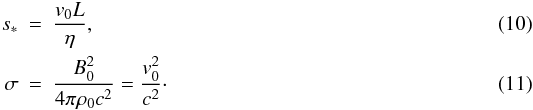 The magnetization parameter σ has been introduced through the displacement current, so that Eq. (8) becomes Eq. (2.4) of Craig & McClymont (1991) when the D’Alembertian −
  is replaced by the Laplacian
  in the limit of σ = 0. It should be noted that v0 represents the Alfvén velocity at radius L only in the nonrelativistic case. The Alfvén velocity at L is in general given by VA ≡ cσ1/2/(σ + 1)1/2 = v0/(σ + 1)1/2. For highly magnetized cases where σ ≫ 1, we have VA ≈ c, whereas VA ≈ v0 for σ ≪ 1. Although Eq. (9) is used for mathematical calculation, the physical results are presented after normalization by VA. The Lundquist number S characterizing the system is defined in terms of the Alfvén velocity VA, the radius L and resistivity η as
  (12)The related parameter s∗ is s∗ = (σ + 1)1/2S.
Equation (9) exhibits two different behaviors near to and far from the origin. For large  , the dissipating term with s∗ can be neglected, so that we have
 ![Mathematical equation: \begin{equation} \left[ - \frac{ \sigma \bar{r}^{2} +1 }{\bar{r}^{2}} \frac{\partial ^{2}}{\partial \bar{t}^{2}} +\bar{\nabla}^{2} \right] \delta A =0. \label{eqn.wave} \end{equation}](/articles/aa/full_html/2011/07/aa16562-11/aa16562-11-eq65.png) (13)This is exactly the equation in the cold plasma limit for propagating a fast magnetoacoustic wave, whose velocity at is given by the Alfvén velocity
(13)This is exactly the equation in the cold plasma limit for propagating a fast magnetoacoustic wave, whose velocity at is given by the Alfvén velocity 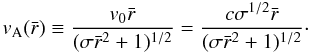 (14)On the other hand, close to the origin, the term with
  can be neglected in Eq. (9). After integrating by
  once, we have
 ![Mathematical equation: \begin{equation} \left[ -\sigma \frac{\partial ^{2}}{\partial \bar{t}^{2}} -\frac{1}{s_{*}} \frac{\partial } {\partial \bar{t}} + \bar{\nabla}^{2} \right] \delta A =0\cdot \label{eqn.tel} \end{equation}](/articles/aa/full_html/2011/07/aa16562-11/aa16562-11-eq69.png) (15)This is the so-called telegraphist’s equation, in which the effect of the finiteness of the velocity c on the resistive losses, or the effect of resistivity on the wave equation, is taken into account. (See, e.g., Morse & Feshbach 1953.) In the limit of σ = 0, the equation becomes the diffusion equation. Thus, Eq. (9) leads to an advection-dominated outer region described by Eq. (13) and a diffusion-dominated inner one described by Eq. (15). The diffusion region may be highly modified in nature for large σ, as electromagnetic wave propagation becomes important even in the diffusion zone for a highly magnetized system. The critical radius
(15)This is the so-called telegraphist’s equation, in which the effect of the finiteness of the velocity c on the resistive losses, or the effect of resistivity on the wave equation, is taken into account. (See, e.g., Morse & Feshbach 1953.) In the limit of σ = 0, the equation becomes the diffusion equation. Thus, Eq. (9) leads to an advection-dominated outer region described by Eq. (13) and a diffusion-dominated inner one described by Eq. (15). The diffusion region may be highly modified in nature for large σ, as electromagnetic wave propagation becomes important even in the diffusion zone for a highly magnetized system. The critical radius  , which separates the two regions, will be determined by the following normal mode analysis.
We solve Eq. (9) as an eigenvalue problem in the form 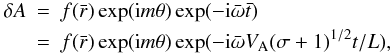 (16)where
  is a complex number. We only consider the axially symmetric m = 0 mode, which is relevant to reconnection at the origin, as discussed in Craig & McClymont (1991). Another type of reconnection for m ≠ 0 is discussed by Ofman et al. (1993) and Vekstein & Bian (2005), but that not is considered here. Equation (9) becomes
 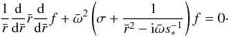 (17)From this, a natural choice of the core radius
  is
is  and corresponds to the usual skin depth (Craig & McClymont 1991). The dissipative term is dominant for
  , whereas outside the critical radius Eq. (17) represents wave propagation, since the term with
  can be neglected. The current density is concentrated around the null point.
A series solution inside the radius  may be expressed as
  (18)where we have normalized to f = 1 at the origin. We solve Eq. (17) with boundary condition (18), from
  to 1, assuming a complex number
  . The boundary condition imposed on the circle
  is f = 0. This means that the magnetic flux is frozen and δE = δj = δv = 0 there. Thus, we have a one-dimensional eigenvalue problem for .
Our main concern is not the whole eigenfrequency spectrum, but rather the lowest frequency mode, which persists for a long time in the magnetic reconnection. In particular, we study the effect of the magnetization parameter on it. For this purpose, we first calculate  for the case σ = 0, and then repeat the calculation, gradually changing the parameter S or σ.
3. Results
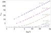 |
Fig. 1 Normalized oscillation time τosc ≡ VAtosc/L as a function of Lundquist number S, for magnetization parameter values σ = 0,10, 102, 103, 103.5, and 104. |
The oscillation time tosc is defined in terms of the real part of the eigenfrequency by  . (A factor (σ + 1)1/2 comes from our normalization of . (See Eq. (16).) Figure 1 shows the normalized time VAtosc/L as a function of S for several values of σ. Craig & McClymont (1991) showed that the relation VAtosc/L ≈ 2lnS ≈ 4.6log S holds for a wide range of S with σ = 0. The origin of this relation can be understood by considering the traveling time of an MHD wave from the outer boundary to the resistive region,
  (19)The velocity in the limit of σ = 0 is scaled by
  , and the dominant contribution in Eq. (19) comes from a small core region. By choosing the lower boundary
  as , we have
  .
.
When σ is included, the oscillation time deviates from the relation VAtosc/L ≈ 2lnS. The normalized time, in general, becomes less than that at σ = 0, as shown in Fig. 1. The logarithmic dependence with S can only be seen in the larger regime, and the coefficient in front of lnS becomes smaller as σ increases. The Alfvén velocity becomes relativistic for σ > 1 at the boundary, and approaches zero toward the center. The velocity becomes nonrelativistic, at the radius  for σ ≫ 1, and the velocity is almost equal to c outside this radius. The wave traveling time in Eq. (19) is almost determined by the slow region inside
  , and the system size may be regarded as being effectively reduced to σ − 1/2L. We therefore have VAtosc/(σ − 1/2L) ≈ 2lnS; i.e., VAtosc/L ≈ 2σ − 1/2lnS for the large S regime. This property can be seen from the curves around log S ≈ 50 in Fig. 1, except for σ = 104. A factor of (σ + 1)1/2 instead of σ1/2 may provide a better extension to σ = 0, but a simple correction is used here.
Figure 1 also shows that VAtosc/L approaches a constant in the small S regime, for sufficiently large σ. Asymptotically the value of this constant as S → 1 is empirically VAtosc/L ≈ ctosc/L ≈ 2.5, which is independent of σ, as long as σ ≥ 102. In our model, the core size increases as  , so the traveling time (19) becomes shorter with decreasing S, but the lower bound is a few times the light crossing time for a region of size L.
The critical value Sc, which discriminates between constant VAtosc/L for smaller S and VAtosc/L ∝ lnS for larger S, is given approximately by lnSc ~ σ1/2, or log Sc ~ 0.4σ1/2. The transition is not very sharp, but the relation does give the approximate boundary between two distinct behaviors. Because log Sc ~ 1 for σ = 10 and log Sc ~ 40 for σ = 104, which are located at the edges of Fig. 1, the two different behaviors are not clearly shown for these parameters. This critical value Sc also characterizes a transition in the decay time as discussed below.
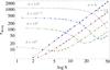 |
Fig. 2 Normalized decay time τdecay ≡ VAtdecay/L as a function of Lundquist number S, for magnetization parameter values σ = 0,10,102,103,103.5, and 104. |
The decay time is related to the imaginary part of ,  . Figure 2 shows the normalized decay time VAtdecay/L as a function of S for several values of σ. The time for σ = 0 scales as VAtdecay/L = 2(lnS)2/π2 (Craig & McClymont 1991). This scaling relation is also broken by the inclusion of σ. The small and large S regimes are different, as they are for the oscillation time. A typical example is given by the curve for σ = 103: the critical value is log Sc ~ 0.4σ1/2 ~ 13 for this case. Logarithmic dependence can be seen for log S > 20, whereas the curve becomes constant for log S < 7. The relation VAtdecay/L ∝ (lnS)2 can be seen in the large S regime, S ≫ Sc, except for σ = 104, but the timescale is reduced to approximately VAtdecay/L ≈ 2σ − 1/2(lnS)2/π2 for σ ≫ 1. The factor σ − 1/2 can be interpreted as being due to an effective reduction of the system’s size, as considered for the oscillation time. The normalized decay time becomes the minimum around Sc.
In the small S regime, S ≪ Sc, normalized decay time approaches a constant value VAtdecay/L ≈ 0.14σ. The normalized decay time for fixed S increases with the magnetization parameter σ. The limit of σ → ∞ corresponds to the vacuum, in which there is no matter (ρ = 0) and the dissipation time becomes infinite. This σ-dependence comes from considering the finiteness of c in the resistive losses. (See Eq. (15).) This effect can be neglected in the large S regime, where the approximation of instantaneous dissipation is good. However, the effect becomes evident in the small S regime.
The energy E of perturbation decreases due to the Ohmic dissipation  (20)The linearized form with Fourier component provides an expression of the decay time as
 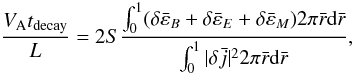 (21)where
  is dimensionless energy density of magnetic field, electric field, kinetic energy of the fluid, and
  is dimensionless current density. Their explicit forms are given by
 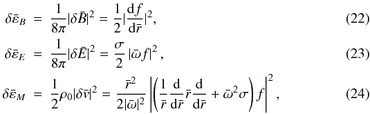 and
and  (25)Spatial distributions of these energy densities are displayed in Fig. 3 for S = 105, σ = 101 and in Fig. 4 for S = 105, σ = 104. These functions are calculated by numerical solution outside
  and by the analytic asymptotic form Eq. (18) inside it. A sharp peak in
  and
and  is located within . Both kinetic energy of matter and magnetic energy are accumulated from the outer part to the core (~
 ), and are dissipated in the central region. However, the distribution of electric energy is flat. These overall features are not so much different in Figs. 3 and 4, although the sharp peak shifts by
 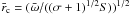 .
.
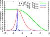 |
Fig. 3 Normalized energy density |


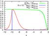 |
Fig. 4 Normalized energy density |

The magnitude of  is much smaller than that of in Fig. 3 (σ = 101), whereas becomes comparable to in Fig. 4 (σ = 104). The electric energy is approximately proportional to σ, as shown in Eq. (23), and it significantly contributes to the sum of energy. As a result, the decay time becomes longer with the increase of σ for fixed S, since the total energy increases. (See Eq. (21).) In the large S regime, however, the functions and are much greater than , so that the electric energy can be neglected. The decay time does not increase with σ in this regime.
4. Discussion and conclusions
Relativistic MHD differs, in general, from the nonrelativistic case in at least three ways: (i) the Lorentz factor γ; (ii) the Coulomb force ρeE; and (iii) the displacement current c-1∂E/∂t in Maxwell’s equation. The Lorentz factor appears in the flow velocity and also in the resistivity of Ohm’s law as a Lorentz contraction. The difference is (v/c)2 in magnitude. Since we considered a linear perturbation from the static state, the inflow velocity is not very high and the Lorentz factor may approximate γ = 1. The magnitude of ρeE is approximately (v/c)2 times the Lorentz force j × B, so is neglected in nonrelativistic MHD. Moreover, the charge density is always zero due to the 2D X-point geometry considered here, so that the Coulomb force ρeE vanishes exactly. This leaves the displacement current as a possible factor in the difference between relativistic and nonrelativistic MHD. We have studied its effects, especially on the dynamics of the magnetic reconnection using a simplified system based on linearized equations in the cold plasma limit. The magnetization parameter σ is incorporated in the basic equation through the displacement current and the oscillation and decay times for the least-damped mode were calculated numerically for parameters S = 10−1050 and σ = 0 − 104.
In the system with σ = 0, for which the displacement current can be neglected, the oscillation and decay times are proportional to lnS and (lnS)2, respectively. By including σ, these timescales are modified in different ways, in two regimes, which are characterized by S ≫ Sc or S ≪ Sc for Sc ≈ exp(σ1/2). For low resistivity, S ≫ Sc, a logarithmic dependence on S can seen, but the timescales normalized by the boundary radius L and the Alfvén velocity VA become smaller with increasing σ. The smaller timescales can be explained as caused by an effective reduction in the size of the system or by the enlargement of the outer region where MHD waves propagate at almost the speed of light, and the traveling time is negligible. On the other hand, for high resistivity, S ≪ Sc, a new feature appears in both the oscillation and decay times, which do not depend on S. The oscillation time is a few times the light crossing time and does not depend on σ. The dissipation time becomes longer in proportion to σ and goes to infinity in the limit of σ → ∞, that is, no dissipation in the vacuum. Reconnection at the X point is thought to be “fast”, since the dissipation time is scaled with (lnS)2. Actual time is on the order of 10–103 times crossing time with Alfvén velocity. The displacement current significantly spoils the good property, and the timescale increases with σ in the high resistive region. The increase in the decay time is related to deficiency of matter, which is involved in the Ohmic dissipation.
Magnetic reconnection is expected to be an important process of abrupt energy release in the solar and magnetar flares; for example, the explosive tearing-mode reconnection in the magnetar like the solar flares is discussed (Lyutikov 2006; Masada et al. 2010). Dimensionless parameters are, however, quite different in them: σ ~ 10-4 and S ~ 1014 in solar corona, whereas it is likely that σ ≫ 1 and S ≫ 1 in a magnetar magnetosphere. The present result in an X-type collapse suggests the dissipation time t ~ 0.1σL/VA ~ 10-5σ (L/106 cm) s in a highly magnetized environment. The spiky rise time (< 0.1 s) or short duration (< 1 s) of the magnetar flare may significantly constrain σL. The energy of the flare ΔE (~1045 erg) should be a part of magnetic energy within the volume L3:  . These two conditions provide an upper limit of σ as σ < 104.5(ρ0/(g/cm3))1/2. In such high-energy events, radiation and possibly pair creation may be important in the energy transfer. Further study of these effects is needed; however, the results in this paper demonstrate that the dynamics significantly depends on the magnetization parameter through the displacement current.
Acknowledgments
This work was supported in part by a Grant-in-Aid for Scientific Research (No. 21540271) from the Japanese Ministry of Education, Culture, Sports, Science and Technology.
References
- Blackman, E. G., & Field, G. B. 1993, Phys. Rev. Lett., 71, 3481 [Google Scholar]
- Craig, I. J. D. 2008, A&A, 487, 1155 [NASA ADS] [CrossRef] [EDP Sciences] [Google Scholar]
- Craig, I. J. D., & McClymont, A. N. 1991, ApJ, 371, L41 [NASA ADS] [CrossRef] [Google Scholar]
- Craig, I. J. D., Litvinenko, Y. E., & Senanayake, T. 2005, A&A, 433, 1139 [NASA ADS] [CrossRef] [EDP Sciences] [Google Scholar]
- Hassam, A. B. 1992, ApJ, 399, 159 [NASA ADS] [CrossRef] [Google Scholar]
- Komissarov, S. S. 2007, MNRAS, 382, 995 [NASA ADS] [CrossRef] [Google Scholar]
- Lyubarsky, Y. E. 2005, MNRAS, 358, 113 [NASA ADS] [CrossRef] [Google Scholar]
- Lyutikov, M. 2006, MNRAS, 367, 1594 [CrossRef] [Google Scholar]
- Lyutikov, M., & Uzdensky, D. 2003, ApJ, 589, 893 [NASA ADS] [CrossRef] [Google Scholar]
- Masada, Y., Nagataki, S., Shibata, K., & Terasawa, T. 2010, PASJ, 62, 1093 [NASA ADS] [Google Scholar]
- McClymont, A. N., & Craig, I. J. D. 1996, ApJ, 466, 487 [NASA ADS] [CrossRef] [Google Scholar]
- McClements, K. G., Thyagaraja, A., Ben Ayed, N., & Fletcher, L. 2004, ApJ, 609, 423 [NASA ADS] [CrossRef] [Google Scholar]
- McLaughlin, J. A., & Hood, A. W. 2004, A&A, 420, 1129 [NASA ADS] [CrossRef] [EDP Sciences] [Google Scholar]
- McLaughlin, J. A., De Moortel, I., Hood, A. W., & Brady, C. S. 2009, A&A, 493, 227 [NASA ADS] [CrossRef] [EDP Sciences] [Google Scholar]
- McLaughlin, J. A., Hood, A. W., & de Moortel, I. 2010, Space Sci. Rev., 62 [Google Scholar]
- Morse, P. M., & Feshbach, H. 1953, Methods of theoretical physics (New York: McGrow-Hill) [Google Scholar]
- Ofman, L., Morrison, P. J., & Steinolfson, R. S. 1993, ApJ, 417, 748 [NASA ADS] [CrossRef] [Google Scholar]
- Vekstein, G., & Bian, N. 2005, ApJ, 632, L151 [NASA ADS] [CrossRef] [Google Scholar]
- Watanabe, N., & Yokoyama, T. 2006, ApJ, 647, L123 [NASA ADS] [CrossRef] [Google Scholar]
- Zenitani, S., & Hoshino, M. 2005, Phys. Rev. Lett., 95, 095001 [NASA ADS] [CrossRef] [PubMed] [Google Scholar]
- Zenitani, S., & Hoshino, M. 2007, ApJ, 670, 702 [NASA ADS] [CrossRef] [Google Scholar]
- Zenitani, S., & Hoshino, M. 2008, ApJ, 677, 530 [NASA ADS] [CrossRef] [Google Scholar]
- Zenitani, S., Hesse, M., & Klimas, A. 2009, ApJ, 696, 1385 [NASA ADS] [CrossRef] [Google Scholar]
All Figures
|
Fig. 1 Normalized oscillation time τosc ≡ VAtosc/L as a function of Lundquist number S, for magnetization parameter values σ = 0,10, 102, 103, 103.5, and 104. |
| In the text | |
|
Fig. 2 Normalized decay time τdecay ≡ VAtdecay/L as a function of Lundquist number S, for magnetization parameter values σ = 0,10,102,103,103.5, and 104. |
| In the text | |
|
Fig. 3 Normalized energy density |
| In the text | |
|
Fig. 4 Normalized energy density |
| In the text | |
Current usage metrics show cumulative count of Article Views (full-text article views including HTML views, PDF and ePub downloads, according to the available data) and Abstracts Views on Vision4Press platform.
Data correspond to usage on the plateform after 2015. The current usage metrics is available 48-96 hours after online publication and is updated daily on week days.
Initial download of the metrics may take a while.