| Issue |
A&A
Volume 569, September 2014
|
|
|---|---|---|
| Article Number | A113 | |
| Number of page(s) | 9 | |
| Section | Stellar structure and evolution | |
| DOI | https://doi.org/10.1051/0004-6361/201424371 | |
| Published online | 01 October 2014 | |
Magnetic activity, differential rotation, and dynamo action in the pulsating F9IV star KIC 5955122
1
INAF, Osservatorio Astrofisico di Catania, via S. Sofia, 78,
95123
Catania,
Italy
e-mail:
alfio.bonanno@inaf.it
2
Leibniz Institute for Astrophysics Potsdam (AIP),
An der Sternwarte
16, 14482
Potsdam,
Germany
3
Stellar Astrophysics Centre, Department of Physics and Astronomy,
Aarhus University, Ny Munkegade
120, 8000
Aarhus C,
Denmark
4
Department of Geoscience, Aarhus University,
Høegh-Guldbergs Gade 2,
8000
Aarhus C,
Denmark
5
Instituut voor Sterrenkunde, KU Leuven, Celestijnenlaan 200D,
3001
Leuven,
Belgium
Received:
11
June
2014
Accepted:
5
August
2014
We present photometric spot modeling of the nearly four-year long light-curve of the Kepler target KIC 5955122 in terms of persisting dark circular surface features. With a Bayesian technique, we produced a plausible surface map that shows dozens of small spots. After some artifacts are removed, the residuals are at ± 0.16 mmag. The shortest rotational period found is P = 16.4 ± 0.2 days. The equator-to-pole extrapolated differential rotation is 0.25 ± 0.02 rad/d. The spots are roughly half as bright as the unperturbed stellar photosphere. Spot latitudes are restricted to the zone ±60° latitude. There is no indication for any near-pole spots. In addition, the p-mode pulsations enabled us to determine the evolutionary status of the star, the extension of the convective zone, and its radius and mass. We discuss the possibility that the clear signature of active regions in the light curve of the F9IV star KIC 5955122 is produced by a flux-transport dynamo action at the base of the convection zone. In particular, we argue that this star has evolved from an active to a quiet status during the Q0–Q16 period of observation, and we predict, according to our dynamo model, that the characteristic activity cycle is of the order of the solar one.
Key words: starspots / stars: rotation / stars: magnetic field / magnetohydrodynamics (MHD) / stars: individual: KIC 5955122 / stars: activity
© ESO, 2014
1. Introduction
The high-quality photometric data from the CoRoT (Baglin et al. 2006) and Kepler (Borucki et al. 2010) space telescopes have opened new possibilities for investigating the origin and evolution of magnetic fields in solar-type stars.
In particular, the possibility of obtaining almost uninterrupted observations for periods much longer than the typical rotation periods has proven to be a key ingredient for characterizing the photometric inhomogeneities and their evolution in young, fast-rotating objects (Fröhlich et al. 2009, 2012, Bonomo & Lanza 2012; Frasca et al. 2011). In solar-like stars the frequency shifts and amplitude modulations in the p-mode spectrum represent an important diagnostic for detecting magnetic activity cycles, as was recently shown for the F5V star HD 49933 (García et al. 2010) and in the subgiant β Hyi (Metcalfe et al. 2007). In these cases a theoretical interpretation of the p-mode spectrum can determine the precise evolutionary status of the star and, in some cases, its internal distribution of angular momentum and the inclination axis as well.
From the theoretical side, it is generally expected that stars with deep convective envelopes (late F, G, K, and early M spectral type) produce a strong radial shear at the interface between the convective zone and the radiative interior, and in fact, numerical simulations of young solar-type stars have clearly demonstrated the possibility of an efficient dynamo action in this case (Augustson et al. 2013). The situation is less clear for early F-type stars where the shallow convection zone makes it unlikely that a large-scale azimuthal field is stored near the surface (Parker 1993). On the other hand, it has been shown (Huber et al. 2011) that the subgiant F5IV-V star Procyon A is significantly more active than the Sun, although its convection zone is only ≈3−4% in radius. A recent work based on a sample of 22 solar-type F stars observed by Kepler has also shown that the activity level in evolved F-stars is in general stronger than expected (Mathur et al. 2014). The key question is therefore which type of dynamo action is at work in this class of objects.
To address this question we have taken advantage of the exquisite quality of Kepler photometry for KIC 5955122, a solar-like F-type pulsator with a clear signature of spot rotational modulation and spot evolution. The key idea is to explicitly build a dynamo model of the magnetic field in this object in the framework of a mean-field approach, and show that its predictions can be compared with the solution of the spot modeling for the photospheric field.
Although this task is in general very difficult, the detection of an acoustic oscillation spectrum in KIC 5955122 is a powerful diagnostic for the stellar interior, and in particular, for the convection efficiency. According to Appourchaux et al. (2012), this object has a p-mode spectrum that is characterized by a large separation Δν = 49.6 μHz, with an excess of power around νmax ~ 826 μHz, which enables estimating the mass, radius, and convective velocities. Because the information on the rotation rate and surface differential rotation is obtained from the spot modeling, reasonable estimates of all the characteristic dynamo numbers are available in this case.
Today, the most promising theoretical framework within which the dynamo action in the Sun is described is the advection-dominated (or flux-transport) dynamo (Dikpati & Gilman 2009; Guerrero & de Gouveia Dal Pino 2009; Bonanno 2013b). According to this idea, the meridional circulation acts as a conveyor belt that transports the magnetic flux toward equatorial latitudes, provided the eddy diffusivity is low enough (Bonanno et al. 2002a). It is then interesting to test this idea on our object because so far its application to a large class of solar-type Mt.Wilson active stars was shown to be problematic (Jouve et al. 2010).
We argue that a flux-transport dynamo can explain several features of the topology and the evolution of the photospheric field in KIC 5955122.
The structure of the paper is as follows: Sect. 1 contains the introduction, in Sect. 2 we describe the observations and data reduction, Sect. 3 describes the Bayesian spot modeling, and Sect. 4 contains the description of the flux-transport dynamo model and a discussion of the numerical results. Section 5 is devoted to the conclusions.
2. Observations of KIC 5955122
2.1. Ground-based data
KIC 5955122 (=TYC 3142-1229-1) has a Kepler magnitude of V = 9.281, Teff = 5747 K, and log g = 4.3 dex according to the Kepler Input Catalog (KIC, Latham et al. 2005). Because it has been shown that the values of Teff given in the KIC are systematically too low for solar-type stars (Pinsonneault et al. 2012), we used spectroscopic data obtained with ESPADONS on April 2010 to derive the stellar astrophysical parameters. We used the code ROTFIT (Frasca et al. 2003, 2006) to evaluate Teff, log g, [Fe/H], and determine vsini. ROTFIT uses a standard χ2 minimization on individual orders using a library of 185 ELODIE archive spectra of standard stars, which covers the space of atmospheric parameters for FGK-type stars with a metallicity above −1 (Prugniel & Soubiran 2001) very uniformly. The result is Teff = 5954 ± 70K, log g = 4.13 ± 0.18dex, [Fe/H]= −0.06 ± 0.12dex, and vsini = 4.4 ± 1.5kms-1. The spectral type is F9IV, which indicates that this is an evolved subgiant.
Another spectroscopic study (Bruntt et al. 2012) instead reported Teff = 5865 ± 60K and log g = 3.88 ± 0.2dex, and vsini = 6.5kms-1 in agreement with the values provided by ROTFIT within the uncertainties. The differences between the values obtained in Bruntt et al. (2012) and the values adopted in this work result in slightly different limb-darkening coefficients, which does not affect the results of the spot modeling in any way, however.
To obtain an asteroseismic estimate of the stellar mass and radius we employed the code Catania-GARSTEC (Bonanno et al. 2002b), following the approach and the physical input described in Metcalfe et al. (2010) for KIC 11026764. In our grid model search we considered the average values from ROTFIT and Bruntt et al. (2012) as astrophysical constraints, and the large separation Δν = 49.6 μHz (Appourchaux et al. 2012) as the main asteroseismic constraint.
The resulting best model has M = 1.12 M⊙, Teff = 5904K, log g = 3.87 dex , Δν = 49.63 μHz, [Fe/H]= −0.11, R = 2.0 R⊙, and an age of 5.223 Gyr. This is very similar to the solution obtained in Metcalfe et al. (2014) using the values of Bruntt et al. (2012) as astrophysical constraints and fitting the individual frequencies. The extension of the convective zone is also very similar to that of the Sun, being rcz = 0.75 R∗. It is thus reasonable to think that in this star a tachocline is also present at the interface between the radiative and convective zones.
Additional observations have been carried out on 26 August 2013 with the high-resolution FIbre-fed Echelle Spectrograph (FIES) mounted on the 2.6 m Nordic Optical Telescope (Frandsen & Lindberg 2000; Telting et al. 2014) to measure the chromospheric activity level. We obtained five spectra with seven-minute exposures using the low-resolution fiber (R = 25 000), which resulted in a signal-to-noise ratio of about 100 at the blue end of the spectrum. Data reduction was performed with FIEStool1 following the basic steps described in Karoff et al. (2013). The values obtained for the Mt. Wilson S-index in the five spectra are S = 0.146,0.181,0.122,0.148,0.142. If we exclude the value of 0.181, which seems to be caused by a cosmic-ray hit in the spectrum, we finally obtain S = 0.140 ± 0.007. Compared with the Sun, the chromospheric emission is similar to that of a quiet Sun, as is apparent from Fig. 1.
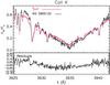 |
Fig. 1 Continuum-normalized observed spectrum (solid black line) in the region between 3925 and 3942 Å (top panel) and between 3960 and 3975 Å (bottom panel) of KIC 5955122, compared with the Sun near the minimum of the activity cycle (HARPS spectrum of Ganymede taken in 2007). |
2.2. Kepler data
The photometric data used in this work were collected by the Kepler photometer in the period from May 2009 to April 2013, corresponding to the run Q0–Q16 for long-cadence data. The light curve was constructed and corrected for according to the method described in Handberg & Lund (2014). Briefly, flux was extracted from target pixel files and bad data points were removed according to the flags from the Kepler team. Only a mild de-trending was applied (τlong = 50 days and τshort = 10 days), with the main effect being the removal of the yearly modulation from the roll of the spacecraft. We refer to Handberg & Lund (2014) for more details on the methodology used for correcting the light curve.
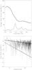 |
Fig. 2 Upper panel: average power density as a function of time in units of the total time for KIC 5955122 (solid line) and for the Sun (dashed line). A prominent peak around 0.36 (in units of the total time) is seen for the Sun and corresponds to the maximum of solar cycle 23. Lower panel: power density at the maximum of the upper figure for KIC 5955122 (continuous line) and for the Sun (dashed line, fit to the power density). Note that in Eq. (1) β = 1 / 2 for KIC 5955122 and β = 2 for the Sun. |
It is interesting to study the time evolution of the power spectral density in the
low-frequency region. We divided the full observational run into chunks of 20 days (a
convenient time interval about the same length as the rotational period, as can be easily
seen by direct inspection of the light curve) and computed the photometric power spectral
density PSD(ν) in each interval. As argued in Huber et al. (2011), this quantity is proportional to
the fractional area covered by active regions, da/a, and to the
luminosity variations δL/L caused by
the flux contrast between the unspotted and spotted stellar areas (Dorren 1987), 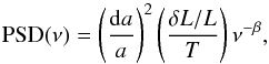 (1)where
β ≈ 2 for
the Sun. The result is shown in Fig. 2, in which we
have plotted the average PSD in the region 5–250 μHz in the top panel as a
function of time in units of the total time of run Q0–Q16 (about four years). During the
first part of the run (mostly during runs Q1 and Q2) there is a clear excess of power that
gradually decreases at later times. For comparison, the dashed line depicts the same
quantity for the Sun for the VIRGO observations in the green channel (Fröhlich et al. 1997), obtained with the SOHO
spacecraft, for the period 1996–2004. In this case, the excess of power is now always
significantly lower than for KIC 5955122, even during the activity maximum of cycle 23,
corresponding of about 0.36 in the normalized time units of the plot. We argue that if
this star has an activity cylce, the evolution of the PSD can be explained as a transition
from a maximum of the activity cycle to a more quiet status (during the Q10–Q16 period)
where the corresponding chromospheric activity S-index is rather low, as expected.
(1)where
β ≈ 2 for
the Sun. The result is shown in Fig. 2, in which we
have plotted the average PSD in the region 5–250 μHz in the top panel as a
function of time in units of the total time of run Q0–Q16 (about four years). During the
first part of the run (mostly during runs Q1 and Q2) there is a clear excess of power that
gradually decreases at later times. For comparison, the dashed line depicts the same
quantity for the Sun for the VIRGO observations in the green channel (Fröhlich et al. 1997), obtained with the SOHO
spacecraft, for the period 1996–2004. In this case, the excess of power is now always
significantly lower than for KIC 5955122, even during the activity maximum of cycle 23,
corresponding of about 0.36 in the normalized time units of the plot. We argue that if
this star has an activity cylce, the evolution of the PSD can be explained as a transition
from a maximum of the activity cycle to a more quiet status (during the Q10–Q16 period)
where the corresponding chromospheric activity S-index is rather low, as expected.
On the other hand, the star is significantly more active during its activity maximum than the Sun. We compare the PSD in the 5–250 μHz region during the maximum in Fig. 2 (upper panel) with the same quantity for the Sun taken at maximum of cycle 23. The result is shown in the lower panel of Fig. 2 where the dashed line, obtained by fitting the PSD decay for the Sun, is to be compared with the solid line obtained for KIC 5955122. In particular, β ≈ 2 in Eq. (1) for the Sun, while β ≈ 0.5 for KIC 5955122.
3. Bayesian spot modeling
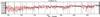 |
Fig. 3 5335 data points from Q0 to Q16 fitted by a 33-spot model (red line). The light curve was divided into 25 parts, whose boundaries are indicated by vertical lines. The residuals are ± 0.16 mmag, i.e., 87.5% of the photometric variance is attributable to dark spots. |
Equation (1) only provides a rough estimate of the excess of power caused by active regions. To characterize the evolution of the photospheric field we discuss in this section a detailed spot model that assumes comparatively long-lived dark features.
3.1. Some general remarks
For actual computations the nearly 60 000 long-cadence data points were combined into bins of 0.25 days width. Each of the 5335 final data points was assigned a weight according to the number of contributing original data points within a bin. Moreover, because the original data show gaps in time in addition to the gaps caused by the measuring quarters Q0 to Q16, the whole data set was accordingly divided into 25 parts (see Fig. 3).
In principle, the spot-modeling procedure is as described in Frasca et al. (2011) and Fröhlich et al. (2012). Central to this parameter estimation is the likelihood function. It measures the probability of the data given a set of parameter values. Because we split the light-curve into parts, the combined likelihood function is the product of the 25 contributions. For each chunk of the light curve a partial likelihood function was constructed as follows: the residuals, given by the deviations between observations and the theoretical model, with measurement errors augmented by systematic (model) errors, were assumed to be Gaussian-distributed in magnitude with unknown variance. Because the data points (bins) were assigned different weights, a data point’s variance scales as the ratio of an unknown variance divided by the number of original data points within the bin. To exclude this unknown variance, the Gaussian likelihood function was integrated over all conceivable values of this unknown variance by applying Jeffreys’ prior, meaning that the unknown variance’s prior behaves like the reciprocal of the variance itself. Afterward, this error-integrated likelihood was additionally integrated over all conceivable magnitude off-sets so that it was not necessary to specify any zero point. Both integrations were made analytically (Fröhlich et al. 2009). It is important to note that each part has its own characteristic error variance and magnitude off-set. Because both quantities are regarded as mere nuisance parameters, they remained undetermined. Only afterward, for presentational purposes, when the data are overplotted on the theoretical light-curve (Fig. 3), the off-sets need to be fixed. This was made by minimizing the distance between the data and the theoretical light-curve.
Theoretical light-curves were computed using the analytical formulae from Dorren (1987) for circular spots, but they were generalized for quadratic limb-darkening (LD).
The two coefficients of the quadratic LD relation were adopted from Claret & Bloemen (2011) assuming an effective temperature of Teff = 5954 K, a gravity of log g = 4.13 dex, and solar metallicity. For the LD no difference was made between the unperturbed photosphere and spots.
Our aim is to analyze the photometric data in terms of a model with lasting dark spots that differ in rotational period to derive at least a lower limit of the amount of differential rotation needed to fit the photometric measurements by a spot model. The spots were allowed to evolve. To estimate the differential rotation we assumed that the spots survive at least a few rotations. Hence, for the sake of simplicity we tried to explain the measured light curve with as low a number of spots as feasible, that is, ideally with the smallest number of free parameters necessary to reach a given fit accuracy. The Bayesian goodness-of-fit by varying the number of free parameters may be quantified by applying the Bayesian information criterion (BIC; Schwarz 1978).
3.2. Search for photometric trains of dips
The light curve (Fig. 3) shows multiple spots. We searched for photometric trains of at least five consecutive dips separated by equal time intervals. The darkening had to exceed 0.5 mmag to be considered a dip in the light curve. This threshold was the only parameter in our train search. The period distribution for trains shown in Fig. 4 for periods between 10 and 30 days seems to be bi-modal. Whether a certain train is due to the cyclic appearance of a physical spot or occurred by chance cannot be decided. We can only conclude from the period distribution the absence of certain spot periods.
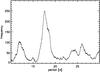 |
Fig. 4 Frequency distribution of train periods. We considered only trains with at least five consecutive dips whose depths exceed 0.5 mmag. |
If there are long-lived spots, at least some trains of spots must be real, that is, be caused by spots that come into view periodically, otherwise the train period distribution would have been much more erratic, as can be proven by a Monte Carlo simulation.
A complication arises because the off-sets of different parts of the light-curve differ. As mentioned before, these off-sets can be only estimated in retrospect. Hence, the period distribution of the trains itself depends somewhat on the anticipated result of the spot modeling.
Periods are most frequently found around 18 and 26 days. The short-period peak (near 12 days) is the second harmonic of the longer-period peak. From the width of the main peak, which covers periods from 16 to 20 days, we derived a lowest value of the differential rotation of 0.08 rad/d. The question arises whether spot periods of the secondary peak around 26 days must be incorporated to derive an acceptable fit for the light curve or not, which results in a much longer differential rotation.
3.3. Details of the spot-modeling procedure
The spot modeling started with the five longest trains with periods around 18 days. While in the search for trains of regularly appearing dips the area evolution of the prospected spots can be arbitrary because the darkening just needs to exceed a certain threshold, the area evolution in the subsequent spot-modeling procedure is specified. Basically, the waxing and waning of spot areas is assumed to evolve linearly with time. Hence, at least four parameters are needed: the largest spot area (expressed in units of the stellar cross-section), the time of largest extent, and two slopes, differing in sign, which describe the increase of the spot area before the time of largest extent and the subsequent decrease. To mitigate the sharp bend at the time when the spot occupies the largest area, another parameter is introduced: the length of a time interval. Within this time interval the actual derivative of the area vs. time relation is linearly interpolated between the two slope values adjacent to this time interval.
As explained in Frasca et al. (2011), it is convenient to use logarithmic quantities to compute posterior probabilites.
A spot central longitude is given with respect to a rigidly rotating coordinate system with an arbitrary period of 18.5 days. We define the longitude as increasing in the direction of stellar rotation, with the zero-point given as the central meridian facing the observer at the beginning of the time series. Two free parameters need to be estimated to describe position and period: the spot longitude at the beginning of the light curve and at the end. The period follows from these two longitude values given the reference period.
The (absolute) latitude of a spot center is computed from the period and the two parameters that specify the law of differential rotation. A simple sin2-ansatz was used (cf. Frasca et al. 2011, Eq. (2)). The two parameters used are sin2(βs) and sin2(βf), where βs and βf describe the latitude of the fastest and of the slowest spot.In principle, our ansatz even includes antisolar rotation in line with the surface rotation profile Ωs(θ), with θ = π/2 − β, which is exploited in Eq. (9) of Sect. 4.1. Here we only considered the solar-like case. Because we are interested in estimating a lower bound on the differential rotation, the fastest spot was fixed to the equator. This reduces the number of free parameters and therefore increases the credibility of the model. The hemisphere to which a spot belongs has to be asserted by trial-and-error.
Additional free parameters are the cosine of the stellar inclination, cos(i), and the common rest intensity, κ, of the spots, which is expressed in units of the surface brightness of the (spotless) star.
Each spot is described by a total of six free parameters. The seventh parameter, which describes the smoothing of the otherwise sharp bend at the time of the largest extent of a spot, was fixed by assuming a smoothing time span of 2.7 days. The hemisphere of the spot may be considered as an eighth parameter.
The likelihood function in the high-dimensional parameter space already matches the posterior probability distribution because the parameters are already represented such that their prior distribution is a flat one in parameter space.
3.4. Enlarging the number of spots
Because it proved impossible to fit the light curve by the effect of a few enduring spots, we considered many spots with lifetimes considerably shorter than the time span of the measurements, but exceeding at least a few rotations. We successively increased the number of spots, and for each added spot ran the adopted Markov chain Monte Carlo (MCMC) procedure anew. A new spot was inserted to match a feature in the light curve that the spot-model so far did not account for. Its initial period was chosen such that adjacent features were accounted for by the new spot as well. We always started with a guess on the period within the interval from 16 to 20 days. Only when this procedure proved to be impossible did we assume a longer initial period. By adding an additional spot, all the other spots that contribute to a periodic darkening in that time span of the light curve have to adjust to the new setting. This is a highly nonlinear problem because many dips are caused by the cumulative effect of more than a single spot. In the end, we obtained a possible solution. This proves that it is at least feasible to interpret the data to some degree within the framework of our model assumptions. There may be a plethora of possible solutions, however. In the worst case, all spots are ephemeral, and interpretating photometric trains in terms of periodically appearing and disappearing spots is misleading. However, with solely ephemeral spots the smoothness of the bi-modal frequency distribution of photometric trains of different periods (Fig. 4) is hardly conceivable. It seems reasonable to expect that at least a few photometrically identified trains are due to a periodic dimming caused by spots that lasted for a few rotations.
3.5. Iterative solution of the 33-spot problem
In many-parameter problems the only feasible way to derive a parameter’s marginal distribution is by applying the MCMC method (Press et al. 2007). To find a relaxed-looking state, an iterative approach was chosen. In one step only the spots contributing to the first half of the time series were allowed to vary while the parameters characterizing the remaining spots were held fixed. In the following step only the spots contributing to the other half were allowed to vary, with the parameters of the remaining spots being those resulting from the step before. This process was iterated several times. This works because the two sets of spots are virtually decoupled, meaning that it results in two relaxed solutions that comprise all spots. In the end, for a given non-spot parameter, for example, differential rotation, both solutions were combined by computing the mean value from both means. The variance of this combined mean follows from the two mean values, which are representative for each half of the time series and the corresponding variances. This seems to be appropriate as long as the parameter space can essentially be reduced to two subspaces. Nevertheless, even by splitting the 33-spot problem into two (comprising 16 and 17 spots, respectively), it is computationally demanding to achieve relaxed MCMC solutions. The results presented were obtained by running up to 128 Markov chains in parallel over many days.
3.6. Results of the spot modeling
With the notable exception of a few singular dips that remain unaccounted for by any persisting dark surface feature, it is possible to fit each major dip in the light curve by the effect of at least one of 33 spots (Fig. 3). Only in about 25% of all cases does the spot period exceed 20 days. The residuals are at 0.16 mmag, which means that ~ 87.5% of the photometric variance can be explained by dark spots.
The result of the Bayesian parameter estimation is the posterior probability distribution across the parameter space. By marginalization, that is, by throwing away the information on correlations between parameters, we derived the marginal distributions of the parameters. Each marginal distribution reveals the probability distribution of a parameter, irrespective of the values that all other parameters may take on. It can be comfortably summarized by its expectation value and credibility interval(s). The most interesting marginal distributions are presented in Figs. 5−9.
We recall that any Bayesian confidence region reflects the elbow room of the underlying theoretical model constrained by the data, nothing else.
3.6.1. Inclination
The photometrically estimated inclination, i, is surprisingly high, nearly 90°. The two marginal distributions of the inclination, computed from the cos(i) parameter, are shown in Fig. 5. The overall inclination, computed from combining the mean values and variances from the two halves of the light curve, is i = 89.0 ± 0.5°.
A cautionary note is in order. The close-to 90° solution for the inclination might in principle be an artifact of the spot modeling. Because of the many spots involved, the hemisphere of a spot cannot be estimated by trial-and-error. To prevent spots from overlapping, the sign of a starting spot latitude was simply assumed to alternate with rising absolute value of the latitude. The only case where the hemisphere of a spot does not matter is in the edge-on (equator) view of the star. Perhaps this is the reason for the preference of a very high inclination.
However, the value of vsini = 6.5kms-1 obtained from Bruntt et al. (2012) with an asteroseismic radius of R ≈ 2 R⊙, yields an inclination of nearly 90°, which is perfectly consistent with the value obtained from the spot modeling.
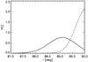 |
Fig. 5 Stellar inclination i from photometry. The solid curve is more representative of the first half of the light curve, the dashed curve more representative of the second half. |
3.6.2. Differential rotation and highest latitudes
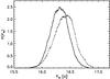 |
Fig. 6 Stellar equatorial rotation period Peq. The solid (dashed) curve is more representative of the first (second) half of the light curve. |
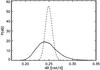 |
Fig. 7 Stellar equator-to-pole differential rotation dΩ. The solid (dashed) curve is more representative of the first (second) half of the light curve. |
A lower limit on the differential rotation of 0.16 rad/d follows from the periods of the fastest (16.4 days) and the slowest spot (27.7 days). When we rely upon the photometrically ill-determined spot latitude, constrained by the period via the parameterized sin2-law of differential rotation, we obtain an extrapolated equator-to-pole differential rotation of 0.25 ± 0.02 rad/d. Both contributing marginal distributions are depicted in Fig. 7. Because the fastest spot was fixed to the equator, its period measures the equatorial rotation period: 16.4 ± 0.2 days (Fig. 6). By a quirk of fate, this equatorial spot proved to be ephemeral. Constituting a train of three consecutive dips and influenced by a fast spot area evolution, the spot rotational period is ill-defined. However, the second -fastest spot, with a period of 16.9 days, is represented in the light curve already by ten consecutive dips. The slowest spot reaches (in the mean) a latitude of ~ 53° (Fig. 8). The corresponding value for the adopted description of the differential rotation reads sin2(βs) = 0.64 ± 0.04, but higher latitudes (up to about 65 degrees) are not excluded. With the exception of periods, all farther reaching conclusions depend on dubious model assumptions, for instance, on the circular shape of the spots, or on the shape of the law of differential surface rotation, and are therefore not as trustworthy as periods.
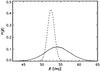 |
Fig. 8 Latitude of the slowest spot. The solid (dashed) curve is more representative of the first (second) half of the light curve. |
3.6.3. Spot intensity
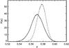 |
Fig. 9 Spot intensity κ with respect to the unspotted photosphere. The solid (dashed) curve is more representative of the first (second) half of the light curve. |
The marginal distribution of the spot rest intensity, expressed in units of the unperturbed stellar surface intensity, κ, is depicted in Fig. 9. According to this, the spots are roughly half as bright as the unspotted stellar photosphere, with κ = 0.57 ± 0.01. Irrespective of the drop in temperature, we applied the same LD prescription to compute the photometric effect of a spot as for the hotter unperturbed surface.
4. Mean field dynamo model
It is reasonable to assume that the flux-transport dynamo can operate in other solar-like stars, although important differences with the solar case might occur for a strong meridional flow or a different rotation rate.
It is convenient to introduce a Reynolds number of the rotation as follows:
 , where R∗ is the stellar
radius and Ωeq is the
equatorial rotation rate. For KIC 5955122 it easy to realize that CΩ is
approximately 1.4 times the solar value. Indeed, the turbulent diffusivity, ηt, scales as the
square of the convective velocities, Ωeq/ Ω⊙ ≈ 1.5 from the
discussion in the previous section, and R∗ ≈ 2 R⊙. By
similar arguments it is possible to estimate that the Reynolds number of the flow,
Cu
=
R∗U/ηt,
with U being
the typical strength of the meridional circulation at the bottom of the convection zone, is
about 1.5 times the solar value
of Cu = 400 (Bonanno 2013b). Note that because the latitudinal
structure of the meridional circulation is still a subject of debate (Zhao et al. 2013; Belucz & Dikpati
2013) we assumed the single-cell model that is most often used in the literature
(Bonanno et al. 2002a; Dikpati & Gilman 2009).
, where R∗ is the stellar
radius and Ωeq is the
equatorial rotation rate. For KIC 5955122 it easy to realize that CΩ is
approximately 1.4 times the solar value. Indeed, the turbulent diffusivity, ηt, scales as the
square of the convective velocities, Ωeq/ Ω⊙ ≈ 1.5 from the
discussion in the previous section, and R∗ ≈ 2 R⊙. By
similar arguments it is possible to estimate that the Reynolds number of the flow,
Cu
=
R∗U/ηt,
with U being
the typical strength of the meridional circulation at the bottom of the convection zone, is
about 1.5 times the solar value
of Cu = 400 (Bonanno 2013b). Note that because the latitudinal
structure of the meridional circulation is still a subject of debate (Zhao et al. 2013; Belucz & Dikpati
2013) we assumed the single-cell model that is most often used in the literature
(Bonanno et al. 2002a; Dikpati & Gilman 2009).
On the other hand, although the typical dynamo numbers of the rotation and meridional circulations are not very different from the solar values, the surface differential rotation is about three times stronger than that of the Sun, and therefore a numerical approach is essential to extract all the relevant information on the topology and dynamics of the toroidal field. This is the main subject of this section.
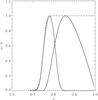 |
Fig. 10 α-effect (solid line), turbulent diffusivity (dot-dashed line), and (minus) the function ψ(x) (dot-dot dashed line) used in the computation. The maximum of the α-effect corresponds to the location of the convective zone. |
4.1. Basic equations
In the following we briefly review the basic ingredients of the advection-dominated
dynamo following the discussion in Bonanno (2013b).
We write the magnetic induction equation as 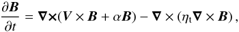 (2)where
ηt is the turbulent diffusivity. In
spherical symmetry the magnetic field B and the mean flow field
V read
(2)where
ηt is the turbulent diffusivity. In
spherical symmetry the magnetic field B and the mean flow field
V read
![\begin{eqnarray} {\vec B} &=& B_\phi(r,\theta,t)\ephi + {\vec \nabla}\times [ A(r,\theta,t) \ephi],\\[2mm] {\vec V} &=& {\vec u}(r,\theta) + r\sin\theta \Omega(r,\theta)\ephi, \end{eqnarray}](/articles/aa/full_html/2014/09/aa24371-14/aa24371-14-eq93.png) where
Bφ(r,θ,φ)êφ
and ∇ × [
A(r,θ,t)êφ
] are the toroidal and poloidal components of the magnetic field. In
this formalism the meridional circulation u(r,θ) and
differential rotation Ω(r,θ) are the poloidal and toroidal components of
the global velocity flow field V. The α-effect is always
antisymmetric with respect to the equator, so that we write
where
Bφ(r,θ,φ)êφ
and ∇ × [
A(r,θ,t)êφ
] are the toroidal and poloidal components of the magnetic field. In
this formalism the meridional circulation u(r,θ) and
differential rotation Ω(r,θ) are the poloidal and toroidal components of
the global velocity flow field V. The α-effect is always
antisymmetric with respect to the equator, so that we write ![\begin{equation} \alpha = \frac{1}{4}\, \alpha_0 \cos\theta\Big [1+{\rm erf}\Bigl(\frac{x-a_{1}}{d}\Bigr)\Big ]\Big [1-{\rm erf} \Bigl(\frac{x-a_{2}}{d}\Bigr)\Big ], \label{aa} \end{equation}](/articles/aa/full_html/2014/09/aa24371-14/aa24371-14-eq98.png) (5)where α0>
0 is the amplitude of the α-effect, x =
r/R⊙ is
the fractional radius, a1 = 0.75, a2 = 0.81 and
d = 0.025
define the location and the thickness of the turbulent layer. We assume that below the
tachocline the turbulent diffusivity is lower by few orders of magnitude than the value
attained in the bulk of the convection zone. We can conveniently represent this transition
with the following functional form:
(5)where α0>
0 is the amplitude of the α-effect, x =
r/R⊙ is
the fractional radius, a1 = 0.75, a2 = 0.81 and
d = 0.025
define the location and the thickness of the turbulent layer. We assume that below the
tachocline the turbulent diffusivity is lower by few orders of magnitude than the value
attained in the bulk of the convection zone. We can conveniently represent this transition
with the following functional form: ![\begin{equation} \label{eta} \eta = \eta_{\rm c} +\frac{1}{2}(\eta_{\rm t} -\eta_{\rm c} )\Bigl[1+{\rm erf}\Bigl(\frac{x-x_{cz}}{d}\Bigr)\Bigr], \end{equation}](/articles/aa/full_html/2014/09/aa24371-14/aa24371-14-eq104.png) (6)where ηt is the eddy
diffusivity, ηc the magnetic diffusivity beneath the
convection zone, and d represents the width of this transition. In
particular, we use the values ηt/ηc =
102, d = 0.02 as for the Sun, with xcz =
0.75 in our case.
(6)where ηt is the eddy
diffusivity, ηc the magnetic diffusivity beneath the
convection zone, and d represents the width of this transition. In
particular, we use the values ηt/ηc =
102, d = 0.02 as for the Sun, with xcz =
0.75 in our case.
The components of the meridional circulation can be represented with the help of a stream
function Ψ(r,θ) = −
sin2θcosθψ(r),
so that 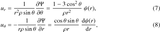 with
the consequence that the condition ∇·(ρu) =
0 is automatically fulfilled. In particular, a positive ψ describes a cell that
circulates clockwise in the northern hemisphere, meaning that the flow is poleward at the
bottom of the convection zone and equatorward at the surface.
with
the consequence that the condition ∇·(ρu) =
0 is automatically fulfilled. In particular, a positive ψ describes a cell that
circulates clockwise in the northern hemisphere, meaning that the flow is poleward at the
bottom of the convection zone and equatorward at the surface.
Following the analysis of the previous section, the differential rotation is assumed to
be solar-like and we write ![\begin{equation} \Omega(r,\theta)=\Omega_{\rm c} +\frac{1}{2}\Bigl[1+\mathrm{erf} \Bigl(\frac{x-x_{cz}}{d_c}\Bigr)\Bigr] \bigl(\Omega_{\rm s}(\theta)-\Omega_{\rm c} \bigr), \quad \label{eq3} \end{equation}](/articles/aa/full_html/2014/09/aa24371-14/aa24371-14-eq115.png) (9)where
Ωc is the uniform
angular velocity of the radiative core, Ωs(θ) = Ωeq −
dΩcos2θ is the latitudinal differential
rotation at the surface, and dΩ =
0.25 rad/d. To estimate Ωc/ Ωeq we used the approach
of Garaud & Guervilly (2009) where the
coupling between radiative interior and convective envelope can be modeled as a spherical
magnetized Couette flow. In our case, this led to Ωc/ Ωeq = (1 − dΩ
/ 3Ωeq) = 0.78 (note that for the Sun
this approximation provides Ωc/ Ωeq = 0.93 as inferred by
helioseismology).
(9)where
Ωc is the uniform
angular velocity of the radiative core, Ωs(θ) = Ωeq −
dΩcos2θ is the latitudinal differential
rotation at the surface, and dΩ =
0.25 rad/d. To estimate Ωc/ Ωeq we used the approach
of Garaud & Guervilly (2009) where the
coupling between radiative interior and convective envelope can be modeled as a spherical
magnetized Couette flow. In our case, this led to Ωc/ Ωeq = (1 − dΩ
/ 3Ωeq) = 0.78 (note that for the Sun
this approximation provides Ωc/ Ωeq = 0.93 as inferred by
helioseismology).
Assuming a standard isotropic mixing-length theory, one can show that to a very good
approximation, (Durney 2000; Bonanno 2013a) the stream function can be described as 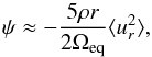 (10)so that it is possible to
determine the stagnation point directly from the underlying stellar model (Bonanno 2013a). Note that a negative ψ describes a flow that is
poleward at the surface and equatorward at the bottom of the convection zone, as we
observe in the Sun. For the actual calculations we employed the following representation
for the stream function:
(10)so that it is possible to
determine the stagnation point directly from the underlying stellar model (Bonanno 2013a). Note that a negative ψ describes a flow that is
poleward at the surface and equatorward at the bottom of the convection zone, as we
observe in the Sun. For the actual calculations we employed the following representation
for the stream function: ![\begin{equation} \psi=C \; \left[1-\exp{\left(-\frac{(x-x_b)^2}{\sigma^2}\right)} \right] (x-1) \; x^2 , \end{equation}](/articles/aa/full_html/2014/09/aa24371-14/aa24371-14-eq123.png) (11)where C is a normalization
factor, xb = 0.75 defines the
penetration of the flow, σ =
0.07 and measures how fast
(11)where C is a normalization
factor, xb = 0.75 defines the
penetration of the flow, σ =
0.07 and measures how fast  decays to zero in the overshoot
layer and the location of the stagnation point. The density profile can be modeled as
decays to zero in the overshoot
layer and the location of the stagnation point. The density profile can be modeled as
 with m = 1.2 and x0 = 0.85,
although our results are not strongly dependent on these values.
with m = 1.2 and x0 = 0.85,
although our results are not strongly dependent on these values.
4.2. Results
We solved Eq. (2) by means of the code CTDYN described in Jouve et al. (2010), which employs a pseudo-spectral decomposition of the induction equation to determine the critical dynamo number Cα = α0R∗/ηt in the kinematic regime (see Jouve et al. 2010 for details).
By scaling the solar dynamo solution discussed in Bonanno (2013b), we have that CΩ ≈ 6 × 10⁴, Cu ≈ 600, and Cα = 6.35, U = 30m / s with ηt = 6.6 × 1011cm2 s-2, and an activity cycle of about 21 years is found.
A typical butterfly diagram for this type of dynamo action is depicted in Fig. 11. It is interesting that there are two branches, one equatorward, another poleward, starting a lower latitude. This is expected because the latitudinal shear is much stronger in this case than for the Sun, and it tends to produce a poleward migration with a positive α-effect in the northern hemisphere. Moreover, the toroidal field belts are confined to latitudes lower than ~ 60° although the α-effect is not suppressed in latitude by the usual ∝sin2θ term.
We intepret this result as a nontrivial confirmation of the analysis of the previous section, according to which spots are distributed mostly below ~ 60° in latitude. We argue that this property is a consequence of a flux-transport dynamo action, which confines the active regions at low latitudes. The predicted length of the activity cycle is perfectly consistent with the possibility, discussed in the first section, that this star has undergone a transition from a maximum of the activity to a quiet state during the Q0–Q16 run.
What happens if we increase the Reynolds number of the flow? In this case, the solution for Cu = 800 is shown in Fig. 12, where the poleward migration clearly dominates. The very narrow and sharp latitudinal extension of the activity region seems not to be strongly supported by our spot model solution, although here polar spots would not be ruled out.
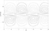 |
Fig. 11 Butterfly diagram for a reference solution with Cα = 6.35, U = 30m / s , ηt = 6.6 × 1011cm2 s-2, and an activity cycle of 21 years. The toroidal field is evaluated at the bottom of the convection zone. The ratio Br/Bφ = 0.0048 at the base of the convection zone. |
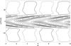 |
Fig. 12 Same parameters as in Fig. 11, but with Cu = 800. In this case, Cα = 7.33, while U = 37m / s. The activity cycle is 17 years. |
5. Conclusions
KIC 5955122 is an interesting laboratory to test the possibility that a flux-transport dynamo is operating in other solar-like stars. The strong modulation observed in the light curve during the Q0-Q16 period can be interpreted as a transition from a very active state, maybe a maximum of the activity, toward a quiet state, as supported by a consistent dynamo model.
Although this star is very evolved, it rotates significantly faster than our Sun, and it is conceivable that during its main-sequence life it has hosted a significant dynamo action. Most probably, its convection zone is still deep enough to produce a strong radial shear at its inner boundary. For this reason (Dikpati & Gilman 2001), the significant toroidal field instabilities are expected to produce an α-effect that can be positive in the northern hemisphere.
On the other hand, we note that the star with an S-index of 0.14 shows only weak chromospheric activity. This could suggest that the dynamos in these evolved F-type stars generally only produce weak chromospheres. This idea is partly supported by the S-indexes as a function of B − V color index measured by Baliunas et al. (1995). Here it is clear that KIC 5955122 with a B − V value of 0.54 is located in a sweet spot where stars with similar color generally show very low chromospheric activity – another star with B − V of 0.54 is Procyon, for example.
Our findings support the idea that the dynamo action in main-sequence and subgiant stars produces photospheric fields that are very different from what is observed in young, fast rotating stars that just approach the zero-age main sequence.
Even though the photospheric field in KIC 5955122 is characterized by a nontrivial topology, the activity cycle is expected to be of the order (or slightly lower) than the solar cycle. This prediction can in fact be falsified with long-term monitoring of the S-index, and we argue that this is an important opportunity to pursue this possibility to test the flux-transport dynamo.
The p-mode pulsations and, in particular, the mixed modes can also provide independent probes of the rotation rate, inclination angle, and possibly upper limits on radial and latitudinal differential rotation. We hope to address these questions in a subsequent paper.
Acknowledgments
We acknowledge the NORDITA dynamo program Differential Rotation and Magnetism across the HR Diagram for providing a stimulating scientific atmosphere. Funding for this Discovery mission is provided by NASA’s Science Mission Directorate. The authors wish to thank the entire Kepler team, without whom these results would not be possible. C.K. acknowledge support from the Villum Foundation. Funding for the Stellar Astrophysics Centre is provided by The Danish National Research Foundation (grant agreement No.: DNRF106). The research is supported by the ASTERISK project (ASTERoseismic Investigations with SONG and Kepler) funded by the European Research Council (grant agreement No.: 267864).
References
- Appourchaux, T., Chaplin, W. J., García, R. A., et al. 2012, A&A, 543, A54 [NASA ADS] [CrossRef] [EDP Sciences] [Google Scholar]
- Augustson, K. C., Brun, A. S., & Toomre, J. 2013, ApJ, 777, 153 [Google Scholar]
- Baglin, A., Auvergne, M., Boisnard, L., et al. 2006, in COSPAR Meeting, 36th COSPAR Scientific Assembly, 36, 3749 [Google Scholar]
- Baliunas, S. L., Donahue, R. A., Soon, W. H., et al. 1995, ApJ, 438, 269 [NASA ADS] [CrossRef] [Google Scholar]
- Belucz, B., & Dikpati, M. 2013, ApJ, 779, 4 [NASA ADS] [CrossRef] [Google Scholar]
- Bonanno, A. 2013a, Geophys. Astrophys. Fluid Dyn., 107, 11 [NASA ADS] [CrossRef] [Google Scholar]
- Bonanno, A. 2013b, Sol. Phys., 287, 185 [NASA ADS] [CrossRef] [Google Scholar]
- Bonomo, A. S., & Lanza, A. F. 2012, A&A, 547, A37 [NASA ADS] [CrossRef] [EDP Sciences] [Google Scholar]
- Bonanno, A., Elstner, D., Rüdiger, G., & Belvedere, G. 2002a, A&A, 390, 673 [NASA ADS] [CrossRef] [EDP Sciences] [Google Scholar]
- Bonanno, A., Schlattl, H., & Paternò, L. 2002b, A&A, 390, 1115 [NASA ADS] [CrossRef] [EDP Sciences] [MathSciNet] [Google Scholar]
- Borucki, W. J., Koch, D., Basri, G., et al. 2010, Science, 327, 977 [NASA ADS] [CrossRef] [PubMed] [Google Scholar]
- Bruntt, H., Basu, S., Smalley, B., et al. 2012, MNRAS, 423, 122 [NASA ADS] [CrossRef] [Google Scholar]
- Claret, A., & Bloemen, S. 2011, A&A, 529, A75 [NASA ADS] [CrossRef] [EDP Sciences] [Google Scholar]
- Dikpati, M., & Gilman, P. A. 2001, ApJ, 559, 428 [NASA ADS] [CrossRef] [Google Scholar]
- Dikpati, M., & Gilman, P. A. 2009, Space Sci. Rev., 144, 67 [NASA ADS] [CrossRef] [Google Scholar]
- Dorren, J. D. 1987, ApJ, 320, 756 [NASA ADS] [CrossRef] [Google Scholar]
- Durney, B. R. 2000, ApJ, 528, 486 [NASA ADS] [CrossRef] [Google Scholar]
- Frandsen, S., & Lindberg, B. 2000, in The 3rd MONS Workshop: Science Preparation and Target Selection, eds. T. Teixeira, & T. Bedding, 163 [Google Scholar]
- Frasca, A., Alcalá, J. M., Covino, E., et al. 2003, A&A, 405, 149 [NASA ADS] [CrossRef] [EDP Sciences] [Google Scholar]
- Frasca, A., Guillout, P., Marilli, E., et al. 2006, A&A, 454, 301 [NASA ADS] [CrossRef] [EDP Sciences] [Google Scholar]
- Frasca, A., Fröhlich, H.-E., Bonanno, A., et al. 2011, A&A, 532, A81 [NASA ADS] [CrossRef] [EDP Sciences] [Google Scholar]
- Fröhlich, C., Andersen, B. N., Appourchaux, T., et al. 1997, Sol. Phys., 170, 1 [NASA ADS] [CrossRef] [Google Scholar]
- Fröhlich, H.-E., Küker, M., Hatzes, A. P., & Strassmeier, K. G. 2009, A&A, 506, 263 [NASA ADS] [CrossRef] [EDP Sciences] [Google Scholar]
- Fröhlich, H.-E., Frasca, A., Catanzaro, G., et al. 2012, A&A, 543, A146 [NASA ADS] [CrossRef] [EDP Sciences] [Google Scholar]
- Garaud, P., & Guervilly, C. 2009, ApJ, 695, 799 [NASA ADS] [CrossRef] [Google Scholar]
- García, R. A., Mathur, S., Salabert, D., et al. 2010, Science, 329, 1032 [NASA ADS] [CrossRef] [PubMed] [Google Scholar]
- Guerrero, G., & de Gouveia Dal Pino, E. M. 2009, Rev. Mex. Astron. Astrofis, 36, 252 [Google Scholar]
- Handberg, R., & Lund, M. N. 2014, MNRAS, accepted [arXiv:1409.1366] [Google Scholar]
- Huber, D., Bedding, T. R., Arentoft, T., et al. 2011, ApJ, 731, 94 [NASA ADS] [CrossRef] [Google Scholar]
- Jouve, L., Brown, B. P., & Brun, A. S. 2010, A&A, 509, A32 [NASA ADS] [CrossRef] [EDP Sciences] [Google Scholar]
- Karoff, C., Metcalfe, T. S., Chaplin, W. J., et al. 2013, MNRAS, 433, 3227 [NASA ADS] [CrossRef] [Google Scholar]
- Latham, D. W., Brown, T. M., Monet, D. G., et al. 2005, in AAS Meeting Abstracts, BAAS, 37, 110.13 [Google Scholar]
- Mathur, S., García, R. A., Ballot, J., et al. 2014, A&A, 562, A124 [NASA ADS] [CrossRef] [EDP Sciences] [Google Scholar]
- Metcalfe, T. S., Dziembowski, W. A., Judge, P. G., & Snow, M. 2007, MNRAS, 379, L16 [NASA ADS] [CrossRef] [Google Scholar]
- Metcalfe, T. S., Monteiro, M. J. P. F. G., Thompson, M. J., et al. 2010, ApJ, 723, 1583 [NASA ADS] [CrossRef] [Google Scholar]
- Metcalfe, T. S., Creevey, O. L., Dogan, G., et al. 2014, ApJ, accepted [arXiv:1402.3614] [Google Scholar]
- Parker, E. N. 1993, ApJ, 408, 707 [Google Scholar]
- Pinsonneault, M. H., An, D., Molenda-Żakowicz, J., et al. 2012, ApJS, 199, 30 [NASA ADS] [CrossRef] [Google Scholar]
- Press, W. H., Teukolsky, S. A., Vetterling, W. T., & Flannery. 2007, Numerical Recipes, 3rd edn. (Cambridge, New York: Cambridge University Press) [Google Scholar]
- Prugniel, P., & Soubiran, C. 2001, A&A, 369, 1048 [NASA ADS] [CrossRef] [EDP Sciences] [Google Scholar]
- Schwarz, G. 1978, Ann. Stat., 6, 461 [NASA ADS] [CrossRef] [MathSciNet] [Google Scholar]
- Telting, J. H., Avila, G., Buchhave, L., et al. 2014, Astron. Nachr., 335, 41 [NASA ADS] [CrossRef] [Google Scholar]
- Zhao, J., Bogart, R. S., Kosovichev, A. G., Duvall, Jr., T. L., & Hartlep, T. 2013, ApJ, 774, L29 [NASA ADS] [CrossRef] [Google Scholar]
All Figures
|
Fig. 1 Continuum-normalized observed spectrum (solid black line) in the region between 3925 and 3942 Å (top panel) and between 3960 and 3975 Å (bottom panel) of KIC 5955122, compared with the Sun near the minimum of the activity cycle (HARPS spectrum of Ganymede taken in 2007). |
| In the text | |
|
Fig. 2 Upper panel: average power density as a function of time in units of the total time for KIC 5955122 (solid line) and for the Sun (dashed line). A prominent peak around 0.36 (in units of the total time) is seen for the Sun and corresponds to the maximum of solar cycle 23. Lower panel: power density at the maximum of the upper figure for KIC 5955122 (continuous line) and for the Sun (dashed line, fit to the power density). Note that in Eq. (1) β = 1 / 2 for KIC 5955122 and β = 2 for the Sun. |
| In the text | |
|
Fig. 3 5335 data points from Q0 to Q16 fitted by a 33-spot model (red line). The light curve was divided into 25 parts, whose boundaries are indicated by vertical lines. The residuals are ± 0.16 mmag, i.e., 87.5% of the photometric variance is attributable to dark spots. |
| In the text | |
|
Fig. 4 Frequency distribution of train periods. We considered only trains with at least five consecutive dips whose depths exceed 0.5 mmag. |
| In the text | |
|
Fig. 5 Stellar inclination i from photometry. The solid curve is more representative of the first half of the light curve, the dashed curve more representative of the second half. |
| In the text | |
|
Fig. 6 Stellar equatorial rotation period Peq. The solid (dashed) curve is more representative of the first (second) half of the light curve. |
| In the text | |
|
Fig. 7 Stellar equator-to-pole differential rotation dΩ. The solid (dashed) curve is more representative of the first (second) half of the light curve. |
| In the text | |
|
Fig. 8 Latitude of the slowest spot. The solid (dashed) curve is more representative of the first (second) half of the light curve. |
| In the text | |
|
Fig. 9 Spot intensity κ with respect to the unspotted photosphere. The solid (dashed) curve is more representative of the first (second) half of the light curve. |
| In the text | |
|
Fig. 10 α-effect (solid line), turbulent diffusivity (dot-dashed line), and (minus) the function ψ(x) (dot-dot dashed line) used in the computation. The maximum of the α-effect corresponds to the location of the convective zone. |
| In the text | |
|
Fig. 11 Butterfly diagram for a reference solution with Cα = 6.35, U = 30m / s , ηt = 6.6 × 1011cm2 s-2, and an activity cycle of 21 years. The toroidal field is evaluated at the bottom of the convection zone. The ratio Br/Bφ = 0.0048 at the base of the convection zone. |
| In the text | |
|
Fig. 12 Same parameters as in Fig. 11, but with Cu = 800. In this case, Cα = 7.33, while U = 37m / s. The activity cycle is 17 years. |
| In the text | |
Current usage metrics show cumulative count of Article Views (full-text article views including HTML views, PDF and ePub downloads, according to the available data) and Abstracts Views on Vision4Press platform.
Data correspond to usage on the plateform after 2015. The current usage metrics is available 48-96 hours after online publication and is updated daily on week days.
Initial download of the metrics may take a while.