| Issue |
A&A
Volume 569, September 2014
|
|
|---|---|---|
| Article Number | A58 | |
| Number of page(s) | 11 | |
| Section | Astrophysical processes | |
| DOI | https://doi.org/10.1051/0004-6361/201423745 | |
| Published online | 24 September 2014 | |
Impact of secondary acceleration on the neutrino spectra in gamma-ray bursts
1
DESY,
Platanenallee 6,
15738
Zeuthen,
Germany
e-mail:
This email address is being protected from spambots. You need JavaScript enabled to view it.
2
Theoretische Physik IV: Plasma-Astroteilchenphysik, Fakultät für
Physik & Astronomie, Ruhr-Universität Bochum, 44780
Bochum,
Germany
e-mail:
This email address is being protected from spambots. You need JavaScript enabled to view it.
3
Lawrence Berkeley National Laboratory,
Berkeley
CA
94720,
USA
e-mail:
This email address is being protected from spambots. You need JavaScript enabled to view it.
4
Department of Physics, University of California,
Berkeley
CA
94720,
USA
Received:
3
March
2014
Accepted:
24
July
2014
Abstract
Context. The observation of charged cosmic rays with energies up to 1020 eV shows that particle acceleration must occur in astrophysical sources. Acceleration of secondary particles like muons and pions, produced in cosmic ray interactions, are usually neglected, however, when calculating the flux of neutrinos from cosmic ray interactions.
Aims. Here, we discuss the acceleration of secondary muons, pions, and kaons in gamma-ray bursts (GRBs) within the internal shock scenario, and their impact on the neutrino fluxes.
Methods. We introduce a two-zone model consisting of an acceleration zone (the shocks) and a radiation zone (the plasma downstream the shocks). The acceleration in the shocks, which is an unavoidable consequence of efficient proton acceleration, requires efficient transport from the radiation back to the acceleration zone. On the other hand, stochastic acceleration in the radiation zone can enhance the secondary spectra of muons and kaons significantly if there is a sufficiently large turbulent region.
Results. Overall, it is plausible that neutrino spectra can be enhanced by up to a factor of two at the peak by stochastic acceleration, that an additional spectral peak appears from shock acceleration of the secondary muons and pions, and that the neutrino production from kaon decays is enhanced.
Conclusions. Depending on the GRB parameters, the general conclusions concerning the limits to the internal shock scenario obtained by recent IceCube and ANTARES analyses may be affected by up to a factor of two by secondary acceleration. Most of the changes occur at energies above 107 GeV, so the effects for next-generation radio-detection experiments will be more pronounced. In the future, however, if GRBs are detected as high-energy neutrino sources, the detection of one or several pronounced peaks around 106 GeV or higher energies could help to derive the basic properties of the magnetic field strength in the GRB.
Key words: acceleration of particles / neutrinos / astroparticle physics / gamma-ray burst: general
© ESO, 2014
1. Introduction
Gamma-ray bursts (GRBs) are a candidate class for the origin of the ultra-high energy cosmic rays (UHECRs). A popular scenario is the internal shock model, where the prompt γ-ray emission originates from the radiation of particles accelerated by internal shocks in the ejected material (Paczynski & Xu 1994; Rees & Meszaros 1994 – see Piran 2004 and Meszaros 2006, for reviews). If a significant baryon flux is accelerated, the GRBs may be a plausible source for the UHECRs. In this case, substantial production of secondary pions, muons, and also kaons are expected from photohadronic interactions between the baryons and the radiation field; these will decay into neutrinos and other decay products (Waxman & Bahcall 1997; Asano & Nagataki 2006). Gamma rays at TeV energies and above are co-produced in the photohadronic process, but are subject to interactions with the internal photon field from the radiation processes, including synchrotron radiation and inverse Compton scattering, in the GRB. The photons are expected to cascade down via pair production cascades so that they can be detected at ~GeV energies. Several such GRBs have been detected be Fermi-LAT (Ackermann et al. 2013), but the associated neutrino production per burst is generally expected to be rather low, see, e.g., Becker et al. (2010). In general, neutrino detection from GRBs with IceCube therefore needs to be done via the stacking of a larger number of bursts, see, e.g., Abbasi et al. (2011, 2012).
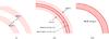 |
Fig. 1 Collision of two shells, illustrated, assuming that they merge (irrelevant for the model presented here). |
Very stringent neutrino flux limits for the internal shock scenario have recently been obtained by the IceCube collaboration using the stacking approach (Abbasi et al. 2011, 2012). Using timing, energy, and directional information for the individual bursts, new limits have been obtained, which are basically background-free and which are significantly below earlier predictions based on gamma-ray observations (Waxman & Bahcall 1997; Guetta et al. 2004; Becker et al. 2006; Abbasi et al. 2010). These predictions have recently been revised from the theoretical perspective (Hümmer et al. 2012; Li 2012; He et al. 2012), yielding an expected flux that is lower by about a factor of ten (Hümmer et al. 2012) depending on the analytical method compared to; see also Adrián-Martí-nez et al. (2013) for an analysis by the ANTARES collaboration using this method. This discrepancy comes mainly from the energy dependence of the proton’s mean free path, the integration over the full photon target spectrum (instead of using the break energy for the pion production efficiency), and several other corrections adding up in the same direction; see Fig. 1 (left) in Hümmer et al. (2012). It should be noted at this point, that the absolute normalization of the neutrino flux scales linearly with the ratio of the luminosity in protons to electrons (baryonic loading). In typical models (Waxman & Bahcall 1997; Guetta et al. 2004; Becker et al. 2006; Abbasi et al. 2010), this ratio is usually assumed to be 10, while theoretical considerations suggest a value of 100 (Schlickeiser 2002) if GRBs are to be the sources of the UHECRs. In a recent study (Baerwald et al. 2014), this value is self-consistently derived from the combined UHECR source and propagation model, including the fit of the UHECR data. For an injection index of two, it has been demonstrated that this value depends on the burst parameters, and that values between 10 and 100 are plausible1. We note that these numbers depend strongly on the proton and electron/photon input spectral shapes and energy ranges, and according to basic theory of stochastic acceleration, it can easily vary between 1000 and 0.1 (Merten & Becker Tjus, in prep.). As also demonstrated in Baerwald et al. (2014), the improved modeling of the GRB spectra can be used to constrain the central parameters of the calculation, i.e., the ratio of protons to electrons and the boost factor. The effects discussed in our study could then contribute to determining another basic property of the GRB, namely the magnetic field strength.
Another argument can be used when relating the neutrino and UHECR fluxes directly if the cosmic rays escape as neutrons produced in the same interactions as the neutrinos (Ahlers et al. 2011). Since this possibility is strongly disfavored (Abbasi et al. 2012) it is conceivable that other escape mechanisms dominate for UHECR escape from GRBs (Baerwald et al. 2013). For instance, if the Larmor radius can reach the shell width at the highest energies, it is plausible that a fraction of the cosmic rays can directly escape. Other possible mechanisms include diffusion out of the shells. In Baerwald et al. (2014), it was demonstrated that even current IceCube data already imply that these alternative escape mechanisms must dominate if GRBs ought to be the sources of the UHECR, and that future IceCube data will exert pressure on these alternative options as well.
The secondary pions, muons, and kaons produced by photohadronic interactions will typically either decay (at low energies) or lose energy by synchrotron radiation (at high energies). At the point where decay and synchrotron timescales are equal, a spectral break in the secondary, and therefore also in the neutrino spectrum is expected. This is the so-called cooling break, see, e.g., Waxman & Bahcall (1997). Additional processes, which potentially affect the secondary spectra, are adiabatic losses, interactions with the radiation field (Kachelriess et al. 2008), and acceleration of the secondaries in the shocks or by stochastic acceleration (Koers & Wijers 2007; Murase et al. 2012; Klein et al. 2013). In this study, we focus on the quantitative impact of the secondary acceleration on the neutrino fluxes, and the conditions for a significant contribution of this effect. A substantial enhancement of the secondary spectra would increase the tension between the recent IceCube observations and the predictions, and would therefore be critical for the interpretation of the recent IceCube results.
2. Model description
The effect of linear acceleration on the secondaries has been discussed in Klein et al. (2013), where it was demonstrated that
significant acceleration effects can be expected if the secondaries can pile up over a large
enough energy range. In GRBs, one has shock (Fermi 1st order) acceleration and, possibly,
stochastic (Fermi 2nd order) acceleration in the plasma downstream the shock if turbulent
magnetic fields are present; see Murase et al.
(2012), where qualitative estimates for the secondary acceleration are made. An
important effect is that the secondaries will be mostly produced by photohadronic
interactions downstream of the shock, where high photon and proton densities are available
over the dynamical timescale of the collision  (as usual, we
refer to quantities in the shock rest frame, SRF, by primed quantities). We therefore
propose a two-zone model:
(as usual, we
refer to quantities in the shock rest frame, SRF, by primed quantities). We therefore
propose a two-zone model:
-
acceleration zone (I):
forward and reverse shocks;
-
radiation zone (II):
plasma downstream the shocks.
The collision of the shells in the internal shock model is illustrated in Fig. 1, where the different zones are shown as well. Although we
do not consider the explicit time dependence, it is a good approximation to use a steady
state model with constant effective densities over the dynamical timescale
. This dynamical
timescale is typically related to the width of the shells Δr′ by
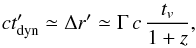 (1)where
tv is the (observed)
variability timescale and Γ is
the appropriately averaged Lorentz boost of the shells, see Kobayashi et al. (1997). We henceforth assume that the adiabatic cooling timescale
is of the same order of magnitude
(1)where
tv is the (observed)
variability timescale and Γ is
the appropriately averaged Lorentz boost of the shells, see Kobayashi et al. (1997). We henceforth assume that the adiabatic cooling timescale
is of the same order of magnitude  .
.
The description of the secondary acceleration in GRBs faces several challenges. First of all, all species (pions, muons, and kaons) may be accelerated. Second, muons are produced by pion decays, which may be accelerated themselves. Third, it is expected that an efficient secondary acceleration is a consequence of the primary (proton, electron) acceleration. The amount of accelerated secondaries depends on the transport between radiation and acceleration zones. And fourth, the spectra of the secondaries, which originate from photohadronic interactions between protons and radiation, are no trivial power laws. It is therefore a priori not clear over what energy range the secondaries could pile up, and what the impact of spectral effects is. Our model aims to address these questions in a way as self-consistently as technically feasible, using state-of-the-art technology.
For the description of the target photon spectrum, we chose a framework relying on gamma-ray observations: it is assumed that the observed gamma-ray spectrum is representative for the spectrum within the source. Based on energy partition arguments, the baryonic and magnetic field densities can be obtained from the gamma-ray spectrum, and the secondary and neutrino fluxes can be computed from the photohadronic interactions between matter and radiation fields, see Guetta et al. (2004), Becker et al. (2006), Abbasi et al. (2010). This framework is slightly different from completely self-consistent (theoretical) approaches generating the target photon spectrum from the radiation processes such as synchrotron radiation and inverse Compton scattering of co-accelerated electrons, or photon production from π0 decays, see e.g., Asano & Meszaros (2011, 2012). The advantage of this approach is that it matches the gamma-ray observations by construction, but the drawback is that it cannot explain them. The overall parameters (photon density, B′) are assumed to be similar for both zones.
We include additional pion and kaon production modes using the methods in Hümmer et al. (2010), based on the physics of SOPHIA (Mücke et al. 2000); see also Murase & Nagataki (2006) for their impact. We also include flavor mixing (Fogli et al. 2012), magnetic field effects on the secondaries, see Kashti & Waxman (2005), Lipari et al. (2007), Baerwald et al. (2011), the kinematics of the weak decays (Lipari et al. 2007), and the recent revisions of the normalization in Hümmer et al. (2012). For details on the underlying model, see Baerwald et al. (2012b). The shape of our neutrino spectra will be different from Waxman & Bahcall (1997), as it is modified by separate cooling peaks for muons, pions, and kaons, additional photo-pion production processes beyond the Δ-resonance, and flavor mixing. This is discussed in detail in Baerwald et al. (2011), where the shape is directly compared to Waxman & Bahcall (1997) for the same GRB parameters. In short, the first break moves to higher energies because it is actually determined by the separate muon cooling break and muon pile-up, whereas the original break at 105 GeV is hardly visible anymore.
Acceleration of protons (zone I)
We assume that protons are accelerated by Fermi shock acceleration in the acceleration zone
to obtain a power law spectrum with spectral index αp ≃ 2. The
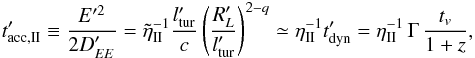
acceleration rate is empirically described, as usual, by (see, e.g., Hillas 1984) ![Mathematical equation: \begin{eqnarray} t'^{-1}_{\mathrm{acc,I}} = \eta_{\rm I} \frac{c}{R_L'} = \eta_{\rm I} \frac{c^2 e B'}{E'} = 9 \times 10^3 \, \eta_{\rm I} \, \frac{B' \, [\text{G}]}{E' \, [\text{GeV}]} \label{equ:accI} \end{eqnarray}](/articles/aa/full_html/2014/09/aa23745-14/aa23745-14-eq17.png) (2)with
the acceleration efficiency 0.1 ≲
ηI ≲ 1 in that definition. Here, the energy
gain is t′−1 ≡
E′−1 | dE′/
dt′ |, ηI corresponds to
the fractional energy gain per cycle, and
(2)with
the acceleration efficiency 0.1 ≲
ηI ≲ 1 in that definition. Here, the energy
gain is t′−1 ≡
E′−1 | dE′/
dt′ |, ηI corresponds to
the fractional energy gain per cycle, and  to the cycle
time.
to the cycle
time.
The acceleration can only be efficient up to the maximum (or critical) energy, where escape
or energy losses start to dominate over the acceleration efficiency. We neglect
photohadronic losses since the considered bursts are optically thin to neutron escape. We
assume that synchrotron or adiabatic losses ( ) limit the maximum
energy, whatever loss rate is larger, or the dynamical timescale. We obtain the maximal
particle energies from
) limit the maximum
energy, whatever loss rate is larger, or the dynamical timescale. We obtain the maximal
particle energies from  as
as ![Mathematical equation: \begin{eqnarray} && E'_{\rm c} \, [\text{GeV}] = \min \left( 2.3 \times 10^{11} \, (m \, [\text{GeV}])^2 \sqrt{\frac{\eta_{\rm I}}{B' \, [\text{G}]}} \, ,\right.\nonumber\\ && \quad \quad \quad \left.9 \times 10^3 \eta_{\rm I} \, B' \, [\text{G}] \, \frac{\Gamma \, t_v \, [\text{s}]}{1+z} \right)\cdot \label{equ:ec} \end{eqnarray}](/articles/aa/full_html/2014/09/aa23745-14/aa23745-14-eq24.png) (3)
(3)
The first entry corresponds to the synchrotron-limited case, and the second entry to the adiabatic loss or dynamical timescale-limited case. We note that Eq. (3) can be applied to the protons as well as the secondaries, at least if they are accelerated by shock acceleration.
The magnetic field can be estimated by energy partition arguments from the observables as
Baerwald et al. (2012b)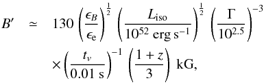 (4)where
ϵB/ϵe
≃ 1 describes equipartition between magnetic field energy and kinetic
energy of the electrons. We note that the variability timescale tv is given in the
observer’s frame at Earth, not in the source (engine) frame.
(4)where
ϵB/ϵe
≃ 1 describes equipartition between magnetic field energy and kinetic
energy of the electrons. We note that the variability timescale tv is given in the
observer’s frame at Earth, not in the source (engine) frame.
Radiation processes and stochastic acceleration of secondaries (zone II)
The protons are injected from the acceleration into the radiation zone with a spectrum
 ,
where Q′ carries units of [ GeV-1 cm-3 s-1
]. In that zone, the protons may interact with photons to produce
secondaries, which undergo synchrotron losses, decay, escape (over the dynamical timescale),
and adiabatic losses, see Winter (2012) for details.
In addition, we consider stochastic acceleration (second order Fermi acceleration) in the
spirit of Murase et al. (2012), following Weidinger & Spanier (2010), Weidinger et al. (2010), Murase et al.
(2012). If there is substantial turbulence, this stochastic (Fermi 2nd order)
acceleration may be important. For the sake of simplicity, we assume that the turbulent
region covers the whole zone II; if only a fraction is affected, only a fraction of
particles will be accelerated and one can trivially obtain the results from our figures.
,
where Q′ carries units of [ GeV-1 cm-3 s-1
]. In that zone, the protons may interact with photons to produce
secondaries, which undergo synchrotron losses, decay, escape (over the dynamical timescale),
and adiabatic losses, see Winter (2012) for details.
In addition, we consider stochastic acceleration (second order Fermi acceleration) in the
spirit of Murase et al. (2012), following Weidinger & Spanier (2010), Weidinger et al. (2010), Murase et al.
(2012). If there is substantial turbulence, this stochastic (Fermi 2nd order)
acceleration may be important. For the sake of simplicity, we assume that the turbulent
region covers the whole zone II; if only a fraction is affected, only a fraction of
particles will be accelerated and one can trivially obtain the results from our figures.
The steady state kinetic equation for the secondary muons, pions, and kaons in zone II is
given by 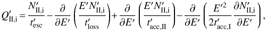 (5)where
 the injection
of species i
from photohadronic processes or parent decays and
the injection
of species i
from photohadronic processes or parent decays and  is the steady
state density (units [ GeV-1
cm-3 ]). The first term on the r.h.s. describes escape by
decay or escape over the dynamical timescale, i.e.,
is the steady
state density (units [ GeV-1
cm-3 ]). The first term on the r.h.s. describes escape by
decay or escape over the dynamical timescale, i.e.,  . The
second term describes energy losses, i.e.,
. The
second term describes energy losses, i.e.,  . Without
acceleration, decay typically dominates at low energies and synchrotron losses at high
energies, and for
. Without
acceleration, decay typically dominates at low energies and synchrotron losses at high
energies, and for  , a
spectral break by two powers is expected. The last two terms in Eq. (5) are characteristic for stochastic acceleration
and always come together with a fixed relative magnitude, see e.g., Weidinger & Spanier (2010), Weidinger et al. (2010).
, a
spectral break by two powers is expected. The last two terms in Eq. (5) are characteristic for stochastic acceleration
and always come together with a fixed relative magnitude, see e.g., Weidinger & Spanier (2010), Weidinger et al. (2010).
We assume that the acceleration timescale  is given by
 (6)following
Murase et al. (2012); see discussion therein. The
energy diffusion coefficient is assumed to be
(6)following
Murase et al. (2012); see discussion therein. The
energy diffusion coefficient is assumed to be  , and
, and
 is the length
scale of the turbulence – which can be estimated from the typical lifetime of the
turbulence. In the third step, we have chosen q ≃ 2 (Murase et al.
2012), and we have re-parametrized the acceleration timescale in terms of the shell
width and turbulence length scale as
is the length
scale of the turbulence – which can be estimated from the typical lifetime of the
turbulence. In the third step, we have chosen q ≃ 2 (Murase et al.
2012), and we have re-parametrized the acceleration timescale in terms of the shell
width and turbulence length scale as  .
.
We expect significant effects of stochastic acceleration if ηII>
1, since then the acceleration exceeds the escape in a certain energy
window. We consider the most extreme case, the kaons, which have the highest energies at
their cooling break. If these are to be accelerated and confined, the condition
 implies that
the stochastic acceleration timescale is longer than the shock acceleration timescale but
shorter than the hydrodynamical timescale. One finds 1 <ηII ≲
10 as a reasonable parameter range; see Eq. (6)2. We
neglect acceleration of the primary protons in zone II, since one can show analytically that
the Fermi 2nd order acceleration only changes the overall normalization of a simple power
law. The proton spectrum normalization is however determined by energy partition arguments,
so the impact of Fermi 2nd order re-acceleration can be absorbed in a re-definition of the
baryonic loading. In addition, the target photon spectrum is based on observation, which
means that we do not need to consider the acceleration of electrons in the spirit of Murase et al. (2012) to describe the prompt emission
spectrum. As in Murase et al. (2012), we assume that
the secondaries in the relevant energy range cannot escape, since
implies that
the stochastic acceleration timescale is longer than the shock acceleration timescale but
shorter than the hydrodynamical timescale. One finds 1 <ηII ≲
10 as a reasonable parameter range; see Eq. (6)2. We
neglect acceleration of the primary protons in zone II, since one can show analytically that
the Fermi 2nd order acceleration only changes the overall normalization of a simple power
law. The proton spectrum normalization is however determined by energy partition arguments,
so the impact of Fermi 2nd order re-acceleration can be absorbed in a re-definition of the
baryonic loading. In addition, the target photon spectrum is based on observation, which
means that we do not need to consider the acceleration of electrons in the spirit of Murase et al. (2012) to describe the prompt emission
spectrum. As in Murase et al. (2012), we assume that
the secondaries in the relevant energy range cannot escape, since
 .
.
Transport of secondaries back to acceleration zone I
Apart from stochastic acceleration in the radiation zone, it is conceivable that a substantial fraction of secondaries is transported back to the acceleration zone I by diffusion. We characterize this fraction as fdiff ≃ λ′/ ΔR′, where λ′ is the diffusion length over the dynamical timescale. Our description closely follows Baerwald et al. (2013) in that aspect, and we assume that the secondaries are produced uniformly over the radiation zone II.
The fraction fdiff of particles which can diffuse back to
the shock front within the dynamical timescale can be estimated from the diffusion length
 as
as 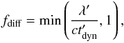 (7)where
 is the spatial
diffusion coefficient. This definition ensures that fdiff ≤ 1. For
example, for Bohm-like diffusion, one has
is the spatial
diffusion coefficient. This definition ensures that fdiff ≤ 1. For
example, for Bohm-like diffusion, one has  and for
Kolmogorov-like diffusion, one has
and for
Kolmogorov-like diffusion, one has  (Stanev 2010; Schlickeiser
2002), and as a consequence,
(Stanev 2010; Schlickeiser
2002), and as a consequence,  and fdiff ∝
E′1 / 6, respectively. As
a lower limit, it can be shown that a fraction
and fdiff ∝
E′1 / 6, respectively. As
a lower limit, it can be shown that a fraction  of the secondaries can
directly escape from the radiation zone in the same way as cosmic rays from the shells
(Baerwald et al. 2013). That is, when the Larmor
radius becomes comparable to the shell width, all particles will reach back to the shocks.
It is therefore reasonable to normalize the transport back to zone I in the way that for
of the secondaries can
directly escape from the radiation zone in the same way as cosmic rays from the shells
(Baerwald et al. 2013). That is, when the Larmor
radius becomes comparable to the shell width, all particles will reach back to the shocks.
It is therefore reasonable to normalize the transport back to zone I in the way that for
 all particles are
efficiently transported3.
all particles are
efficiently transported3.
Muons, pions, and kaons will typically not reach these high energies, since synchrotron
losses lead to a spectral break. As a consequence, only the fraction
 will diffuse back, at the most, where
  is the maximal
energy in Eq. (3). For pions and kaons the
break energies are typically higher than for muons, which means that a larger fraction of
pions and kaons should be transported back to zone I.
is the maximal
energy in Eq. (3). For pions and kaons the
break energies are typically higher than for muons, which means that a larger fraction of
pions and kaons should be transported back to zone I.
We note that stochastic acceleration and the transport by diffusion are connected via
transport theory. Specifically, it is shown in e.g., Schlickeiser (2002), that in the relativistic limit of E ≈
p·c, the product of the spatial and
momentum diffusion coefficients is given as
 (8)where
w is a
constant parameter defining the turbulence scale, which is often included in the definition
of the Alfvén velocity vA (see, e.g., Gebauer 2010, for a summary). The wave spectrum follows a
power law ka with the index
a connected
to the spatial diffusion coefficient as Dxx ∝ E′2−a. For Kolmogorov-type diffusion,
a = 5/3, while in the Bohm-case, a = 1. This means that efficient stochastic
acceleration
(8)where
w is a
constant parameter defining the turbulence scale, which is often included in the definition
of the Alfvén velocity vA (see, e.g., Gebauer 2010, for a summary). The wave spectrum follows a
power law ka with the index
a connected
to the spatial diffusion coefficient as Dxx ∝ E′2−a. For Kolmogorov-type diffusion,
a = 5/3, while in the Bohm-case, a = 1. This means that efficient stochastic
acceleration  in zone II, see Eq. (6), implies inefficient
spatial transport, and vice versa. In particular, if
in zone II, see Eq. (6), implies inefficient
spatial transport, and vice versa. In particular, if  , as we assumed
above,
, as we assumed
above,  .
Therefore, q ~
2 is roughly consistent with Kolmogorov diffusion, which we use as a
standard in the following. It is conceivable from this discussion that the acceleration of
the secondaries dominates either in zone I or zone II as a function of energy, depending on
the efficiency of transport back to the acceleration zone versus stochastic acceleration.
.
Therefore, q ~
2 is roughly consistent with Kolmogorov diffusion, which we use as a
standard in the following. It is conceivable from this discussion that the acceleration of
the secondaries dominates either in zone I or zone II as a function of energy, depending on
the efficiency of transport back to the acceleration zone versus stochastic acceleration.
Shock acceleration of secondaries in zone I
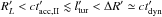
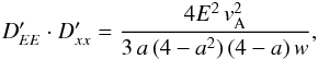
The injection from the radiation back into the shock zone is given by 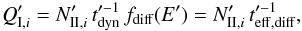 (9)where
one can define the effective diffusion timescale
(9)where
one can define the effective diffusion timescale  . We note that
 is the
ejected spectrum if all particles can escape from zone II over the dynamical timescale,
whereas fdiff ≤
1 characterizes the energy-dependent fraction obtained from Eq. (7). In addition, note that
is the
ejected spectrum if all particles can escape from zone II over the dynamical timescale,
whereas fdiff ≤
1 characterizes the energy-dependent fraction obtained from Eq. (7). In addition, note that
 ,
so diffusion is always less efficient than the adiabatic cooling or escape over the
dynamical timescale in zone II, and is therefore not included in Eq. (5).
,
so diffusion is always less efficient than the adiabatic cooling or escape over the
dynamical timescale in zone II, and is therefore not included in Eq. (5).
The corresponding kinetic equation for the secondaries in zone I is given in the steady
state by  (10)with
the same acceleration efficiency as for the protons Eq. (2). That is, we assume that the secondaries undergo acceleration similar
to the protons, suffer from synchrotron losses, and escape via decay and escape from the
acceleration zone over the dynamical timescale, i.e.,
(10)with
the same acceleration efficiency as for the protons Eq. (2). That is, we assume that the secondaries undergo acceleration similar
to the protons, suffer from synchrotron losses, and escape via decay and escape from the
acceleration zone over the dynamical timescale, i.e.,
 . Since
 in order to have significant secondary acceleration (both have the same energy dependence),
the particles at the highest energies can typically escape over the dynamical timescale from
zone I before they decay. Therefore, we assume that accelerated secondaries decay in the
radiation zone4.
in order to have significant secondary acceleration (both have the same energy dependence),
the particles at the highest energies can typically escape over the dynamical timescale from
zone I before they decay. Therefore, we assume that accelerated secondaries decay in the
radiation zone4.
One may ask if this approach is consistent with the textbook version of Fermi shock
acceleration. In that version, the proton index is given by αp =
Pesc/ηI +
1, where Pesc is the (constant) escape probability
per cycle and η
is the (constant) fractional energy gain per cycle. The ratio Pesc/ηI = 3
/ (χ−1) ≃ 1 depends on the
compression ratio χ only, where χ ≃ 4 for a strong shock. As
a consequence, a “intrinsic” escape term  is needed for a self-consistent kinetic simulation. In our approach, we checked analytically
and numerically that such an additional escape term
is needed for a self-consistent kinetic simulation. In our approach, we checked analytically
and numerically that such an additional escape term 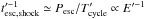 with Pesc =
ηI and
with Pesc =
ηI and
 produces
an E′ −
2 ejection spectrum for the protons if a narrow-energetic particle
distribution is injected. Here, it is crucial that acceleration and escape terms carry the
same energy dependence (which is implied by the constant energy gain and escape probability
per cycle), and that
produces
an E′ −
2 ejection spectrum for the protons if a narrow-energetic particle
distribution is injected. Here, it is crucial that acceleration and escape terms carry the
same energy dependence (which is implied by the constant energy gain and escape probability
per cycle), and that  , which means that
 and
N′
have different energy dependencies. For the secondaries, such an escape term will suppress
the spectra somewhat, depending on the spectral index of the injection (determined by the
ratio Pesc/ηI).
For the sake of simplicity, we assume that the secondaries will escape via decay or over the
dynamical timescale only. This is in a way the most aggressive assumption one can make,
which will however support our conclusions. It may also apply if the escape properties
change over time, the acceleration site of the secondaries is different from the one of the
primaries, or if the secondaries, which have lower energies than the protons, are trapped in
magnetic fields, whereas the protons are injected into the shock at relatively high energies
with a larger Larmor radius.
and
N′
have different energy dependencies. For the secondaries, such an escape term will suppress
the spectra somewhat, depending on the spectral index of the injection (determined by the
ratio Pesc/ηI).
For the sake of simplicity, we assume that the secondaries will escape via decay or over the
dynamical timescale only. This is in a way the most aggressive assumption one can make,
which will however support our conclusions. It may also apply if the escape properties
change over time, the acceleration site of the secondaries is different from the one of the
primaries, or if the secondaries, which have lower energies than the protons, are trapped in
magnetic fields, whereas the protons are injected into the shock at relatively high energies
with a larger Larmor radius.
3. Impact of acceleration effects on the secondaries
Properties of four bursts discussed in this study.
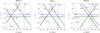 |
Fig. 2 Relevant inverse timescales for secondary muons, pions, and kaons (in the different panels) as a function of the secondary energy in the SRF. The chosen acceleration rate for zones I and II are ηI = 0.1 and ηII = 2.5, respectively. The burst parameters correspond to the Standard Burst in Table 1. |
In order to illustrate the impact of the acceleration on the secondaries, we choose the GRB
parameters listed in the second column of Table 1 for
a burst chosen to reproduce the properties of the Waxman-Bahcall burst (Waxman & Bahcall 1997; Waxman & Bahcall 1999; plateau between 105 and 107 GeV in
 ), see Baerwald et al. (2011). The corresponding inverse
timescales are shown in Fig. 2 for the secondary muons,
pions, and kaons (in the different panels, in SRF). We can use this figure to discuss the
expected behavior in the different zones.
), see Baerwald et al. (2011). The corresponding inverse
timescales are shown in Fig. 2 for the secondary muons,
pions, and kaons (in the different panels, in SRF). We can use this figure to discuss the
expected behavior in the different zones.
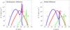 |
Fig. 3 Effect of shock acceleration on steady state densities N′ of muons, pions, and kaons for two different transport mechanisms between radiation and acceleration zone (different panels, in SRF). The plots use the burst SB from Table 1 and ηI = 0.1. The dashed curves are shown without acceleration for comparison. |
In the acceleration zone (I), acceleration or synchrotron losses dominate for all species.
The maximal (critical) energy can be obtained from Eq. (3) as for protons, where adiabatic losses are also included as a
possibility to limit the maximal energy. From the figure it is clear that it is close to
each other for muons and pions, whereas it is significantly higher for kaons. Here, all
secondary species can be, in principle, efficiently accelerated in the shock, since
 .
The largest difference between decay and acceleration, which have the same energy
dependence, is obtained for muons, the smallest for kaons. Therefore, one may expect that
muons are most efficiently accelerated, see also Klein et
al. (2013).
.
The largest difference between decay and acceleration, which have the same energy
dependence, is obtained for muons, the smallest for kaons. Therefore, one may expect that
muons are most efficiently accelerated, see also Klein et
al. (2013).
The pile-up depends on the energy efficiency range of the acceleration. For GRBs, that is
non-trivial to determine, since the secondary spectrum has a spectral break coming from the
gamma-ray spectrum; hence the potential pile-up range is given by the interval between that
break and the critical energy. Another break, the synchrotron cooling break, can be obtained
from  , and is
lowest for muons and highest for kaons. It shows up in all cases at lower energies than
Ec. Even more complicated, the critical energy
is above the cooling break in all cases, which means that its energy is beyond the peak
energy of the spectrum, and that it is not guaranteed that the peak flux of the spectrum
will be increased at the absolute maximum. We note that it is not simply possible to lower
the magnetic field to reduce the cooling and enhance the effect of the acceleration, since
the acceleration efficiency will be reduced, whereas the cooling break will persist as
adiabatic cooling break even if synchrotron losses are suppressed (where
, and is
lowest for muons and highest for kaons. It shows up in all cases at lower energies than
Ec. Even more complicated, the critical energy
is above the cooling break in all cases, which means that its energy is beyond the peak
energy of the spectrum, and that it is not guaranteed that the peak flux of the spectrum
will be increased at the absolute maximum. We note that it is not simply possible to lower
the magnetic field to reduce the cooling and enhance the effect of the acceleration, since
the acceleration efficiency will be reduced, whereas the cooling break will persist as
adiabatic cooling break even if synchrotron losses are suppressed (where
 ). We
will however discuss the conditions for the possibly largest acceleration effects in the
next section.
). We
will however discuss the conditions for the possibly largest acceleration effects in the
next section.
As far as the transport between radiation zone, where the secondaries are mostly produced,
and the acceleration zone is concerned, we show the effective diffusion rates
 (see Eq. (9)) for the Kolmogorov and Bohm
cases in the figure as upper and lower dashed curves, respectively. It is clear that the
higher the critical energy, the more particles will be transported back to the shock.
Therefore, the transport is expected to be most efficient for kaons, which somewhat
compensates for the less efficient acceleration – depending on the transport type. The
Kolmogorov and Bohm cases give the range of plausible transport scenarios. Perfect transport
(all particles transported back to the shock over the dynamical timescale) would correspond
to
(see Eq. (9)) for the Kolmogorov and Bohm
cases in the figure as upper and lower dashed curves, respectively. It is clear that the
higher the critical energy, the more particles will be transported back to the shock.
Therefore, the transport is expected to be most efficient for kaons, which somewhat
compensates for the less efficient acceleration – depending on the transport type. The
Kolmogorov and Bohm cases give the range of plausible transport scenarios. Perfect transport
(all particles transported back to the shock over the dynamical timescale) would correspond
to  .
As most conservative assumption, only the particles not scattering at all may reach back to
the shock, corresponding to the direct escape in Baerwald et
al. (2013). In that case, the transport is only efficient if the Larmor radius
reaches the size of the region. We checked that the results for the Kolmogorov case are
already quite similar to the perfect transport case, whereas the Bohm case and steeper
energy dependencies lead to very small amounts of secondary acceleration, see below.
.
As most conservative assumption, only the particles not scattering at all may reach back to
the shock, corresponding to the direct escape in Baerwald et
al. (2013). In that case, the transport is only efficient if the Larmor radius
reaches the size of the region. We checked that the results for the Kolmogorov case are
already quite similar to the perfect transport case, whereas the Bohm case and steeper
energy dependencies lead to very small amounts of secondary acceleration, see below.
For the stochastic acceleration in zone II, the largest effects are expected if
 dominates over the synchrotron and decay timescales in the radiation zone. Because of the
shallow dependence on energy, a small window (about one order of magnitude in energy) can be
found for muons and kaons in Fig. 2, whereas pions are
hardly affected for the chosen acceleration efficiency. In summary, we expect the most
interesting results for muons, which may be efficiently accelerated in both zones, and
kaons, which may be efficiently transported back to the shock and efficiently accelerated in
the radiation zone.
dominates over the synchrotron and decay timescales in the radiation zone. Because of the
shallow dependence on energy, a small window (about one order of magnitude in energy) can be
found for muons and kaons in Fig. 2, whereas pions are
hardly affected for the chosen acceleration efficiency. In summary, we expect the most
interesting results for muons, which may be efficiently accelerated in both zones, and
kaons, which may be efficiently transported back to the shock and efficiently accelerated in
the radiation zone.
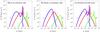 |
Fig. 4 Effect of shock acceleration, stochastic acceleration, and both accelerations combined (in different panels) on steady state densities N′ for muons, pions, and kaons. Here, the burst SB from Table 1, ηI = 0.1, and ηII = 2.5 have been used. The different panels are for acceleration in the shock (left), in the radiation zone (middle), and both (right). Here, Kolmogorov diffusion has been used as transport mechanism between the two zones. The dashed curves are shown without acceleration for comparison. |
These qualitative considerations are quantitatively supported by numerical simulations. We
focus in Fig. 3 first, where the effect of shock
acceleration is shown on the secondary muons, pions, and kaons. This figure shows the steady
state spectra N′, which differ in shape from the neutrino
ejection spectra; see also Appendix A in Baerwald et al.
(2012b). Solving Eq. (5) for decay
only, one obtains  below the peak of
the spectra. Therefore, Q′ ∝
(E′)-2 for N′ ∝
(E′)-1, which can be compared to
the neutrino ejection spectra in terms of shape.
below the peak of
the spectra. Therefore, Q′ ∝
(E′)-2 for N′ ∝
(E′)-1, which can be compared to
the neutrino ejection spectra in terms of shape.
The left panel in Fig. 3 uses Kolmogorov diffusion from the radiation to the acceleration zone, the right panel Bohm diffusion, where these may be regarded as the optimistic and conservative cases for the transport. The shock acceleration leads to the pile-up spikes at the critical energies, marked in Fig. 2, which are also observed in Klein et al. (2013). The acceleration components are most prominent for Kolmogorov diffusion, where many secondaries are transported back to the shock, and least prominent for the Bohm diffusion. As we discussed above, because of the balance between transport and acceleration efficiency, muons and kaons are mostly accelerated, whereas the effect on the pions is smaller.
In either case, the spikes in the muon or pion spectra are washed out in the neutrino spectrum, because the kinematics of the weak decays re-distributes the energies of the parent. The spikes lead to shoulders in the neutrino spectra, as can be seen in Fig. 5. Most importantly, the effect of muon acceleration may be shadowed by the regular pion spectrum, as it is evident from the right panel. Therefore, in the Bohm case, the effect of acceleration on the neutrinos is hardly visible. In the Kolmogorov case, on the other hand, two distinctive peaks (from pion/muon acceleration and from kaon acceleration) should be visible, where the one from pion/muon acceleration is closest to the overall peak of the spectrum and therefore perhaps easiest to detect. In the following, we will only discuss the transport by Kolmogorov diffusion, which may be optimistic but is the minimum requirement to observe significant effects on the neutrino spectra. As a minor detail, in Fig. 3, left panel, a small enhancement can be seen above the critical energy for muons, which comes from the fact that some of the muons are injected above the critical energy from accelerated pions.
Apart from shock acceleration of secondaries transported back to the shock, stochastic acceleration in a turbulent radiation zone could be relevant. In order to maximize the effect, we assume that the whole radiation zone is turbulent, and show the impact of shock acceleration (left panel), stochastic acceleration (middle panel), and acceleration in both zones (right panel) in Fig. 4. As discussed above, stochastic acceleration can lead to a significant enhancement of the muon and kaon spectra at their peaks, where stochastic acceleration is efficient over about one order of magnitude in energy for the chosen acceleration efficiency. The combined effect of acceleration in both zones is shown in the right panel, and is (to a first approximation) an addition of the two effects. One could in principle assume even somewhat more extreme acceleration efficiencies in zone II, which leads to a much stronger enhancement. However, current neutrino data (Abbasi et al. 2012) already puts constraints on scenarios with more optimistic secondary acceleration.
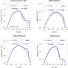 |
Fig. 5 Effect of acceleration on the muon neutrino fluences in the observer’s frame for the bursts in Table 1. Here, ηI = 0.1 and ηII = 2.5 have been assumed, as well as Kolmogorov diffusion as transport mechanism between zones II and I. Here, “No acc.” refers to no acceleration of the secondaries, “Shock” to shock acceleration in zone I only, “Stochastic” to stochastic acceleration in zone II only, and “Both” to the combined effect in both zones. The flavor mixing has been computed with the parameters in Fogli et al. (2012). |
4. Impact on neutrino fluences
The upper left panel of Fig. 5 shows the neutrino spectra for the standard burst from Table 1. In the muon neutrino fluence, the enhancement of the peaks from muon and kaon decays in the case of stochastic acceleration can be clearly seen. For the shock acceleration, the spikes in Fig. 4 translate into peaks at energies higher by a factor of Γ / (1 + z). The combined effect enhances the neutrino spectrum by about 50% in that case, leading to an additional peak at about 108 GeV, and increases the neutrino peak from kaon decays significantly. The spiky secondary particle spectra lead to E-1 spectra for the neutrinos, since the kinematics of weak decays cannot exceed this spectral index.
It is, of course, an interesting question how much these observations depend on the parameter values. We therefore choose three different observations, recently observed (by Fermi) GRBs, as examples: GRB 080916C, GRB 090902B, and GRB 091024. GRB 080916C is one of the brightest bursts ever seen, although at a large redshift, and one of the best studied Fermi-LAT bursts. The gamma-ray spectrum of GRB 090902B has a relatively steep cutoff, and might therefore be representative for a class of bursts for which the gamma-ray spectrum can be fit with a single power law with exponential cutoff as well. GRB 091024 can be regarded as a typical example representative for many Fermi-GBM bursts (Nava et al. 2011), except for the long duration. We note that GRB 080916C and GRB 090902B have an exceptionally large Γ ≳ 1000, whereas Γ ≃ 200 for the last burst. All three observed bursts have in common that the required parameters for the neutrino flux computation can be taken from the literature; see the Table 1 and its caption for the references. We note that these bursts have been also studied in the context of neutrino decays (Baerwald et al. 2012a) and the normalization question (Hümmer 2013; Winter 2012).
We show in Fig. 5 the neutrino spectra for the four representative GRBs listed in Table 1, The effects of the secondary acceleration on the neutrino spectra are depicted in Fig. 5. To a first approximation, the effects are dominated by the strength of the magnetic field strength, which can be estimated with Eq. (4). GRB 091024 has a similar magnetic field (about 60 kG) to our Standard Burst (about 290 kG), whereas the magnetic fields for GRB 080916C (4 kG) and GRB 090902B (6 kG) are significantly lower because of their large Lorentz boosts. Consequently, the spectral shapes of the neutrino spectra are very different, dominated by an adiabatic cooling break which changes the spectrum only by one power. In these cases, it is possible that the stochastic and shock acceleration effects add up.
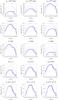 |
Fig. 6 Effect of acceleration on the muon neutrino fluences in the observer’s frame for the burst “SB” in Table 1 with some parameters changed, as indicated in the panel captions. The color codings are the same as in Fig. 5. For reference, the standard burst (curve for acceleration in both zones) is shown in light gray in all panels. We note that the vertical axes have different scalings in the different rows. |
In Fig. 6, we present a further variation of the
parameters for the burst “SB”, as given in the individual panel captions, choosing some more
extreme values. For comparison, we also included the standard values as gray curves
(acceleration in both zones). First of all, note that the normalization of the neutrino
fluences roughly scales with the pion production efficiency ∝ (see Waxman & Bahcall 1997; Guetta et
al. 2004) times T90, while the photon spectral indices
have a smaller impact (the photon spectrum is normalized to the observed fluence). The
secondary acceleration effects are qualitatively similar to the standard case for
T90 and the photon spectral indices, as the
magnetic field is hardly affected. For Liso, tv, and Γ, however, there can be qualitative
differences, which are consistent with our conclusions. One noteworthy exception might be
the case of Γ = 800 (third row,
third column), where the combined acceleration effect leads to a clear peak at about
109 GeV. However,
note that the total normalization is significantly reduced, as the interaction region (and
therefore particle densities) is much smaller in the shock rest frame.
(see Waxman & Bahcall 1997; Guetta et
al. 2004) times T90, while the photon spectral indices
have a smaller impact (the photon spectrum is normalized to the observed fluence). The
secondary acceleration effects are qualitatively similar to the standard case for
T90 and the photon spectral indices, as the
magnetic field is hardly affected. For Liso, tv, and Γ, however, there can be qualitative
differences, which are consistent with our conclusions. One noteworthy exception might be
the case of Γ = 800 (third row,
third column), where the combined acceleration effect leads to a clear peak at about
109 GeV. However,
note that the total normalization is significantly reduced, as the interaction region (and
therefore particle densities) is much smaller in the shock rest frame.
One may ask the question when these largest effects can be expected and if they can be
enhanced. The peak of the secondary spectrum in E2N′ is given
by the cooling break  . The
critical energy for the shock acceleration is typically given by
. The
critical energy for the shock acceleration is typically given by
 .
The critical energy for the stochastic acceleration is determined by
.
The critical energy for the stochastic acceleration is determined by
 ,
which means that stochastic acceleration can be efficient up to relatively large energies
for small B′ (as one can see in the figure). If the
stochastic and shock acceleration criticial energies do not conincide, one therefore expects
the maximal enhancement effect at the peak for
,
which means that stochastic acceleration can be efficient up to relatively large energies
for small B′ (as one can see in the figure). If the
stochastic and shock acceleration criticial energies do not conincide, one therefore expects
the maximal enhancement effect at the peak for  ,
where the cooling break and critical energy for shock acceleration are equal. This condition
translates into a critical magnetic field,
,
where the cooling break and critical energy for shock acceleration are equal. This condition
translates into a critical magnetic field,
![Mathematical equation: \begin{eqnarray} B_{\rm c}' \simeq 10^{-4} \, \eta_{\rm I}^{-1} \frac{m \, [\mathrm{GeV}]}{\tau_0 \, [\mathrm{s}]} \, \mathrm{G}, \end{eqnarray}](/articles/aa/full_html/2014/09/aa23745-14/aa23745-14-eq148.png) (11)where
m is the mass
of the secondary and τ0 its rest-frame lifetime. The ratio
m/τ0 ≃ 4.8 ×
104 GeV s-1 is smallest for muons, where
(11)where
m is the mass
of the secondary and τ0 its rest-frame lifetime. The ratio
m/τ0 ≃ 4.8 ×
104 GeV s-1 is smallest for muons, where
 (for ηI = 0.1). Since
for muons, the acceleration is most efficient, the pions and kaons will rather decay than
being accelerated in that case. The closest parameters can be found for the GRBs with high
Lorentz factors (to achieve high energies) and relatively low magnetic fields GRB 080916C
and GRB 090902B, best seen in the lower-left panel of Fig. 5 as an additional peak only a slightly above the energy of the absolute maximum.
In principle, one can also find such a critical magnetic field for kaons, for which
m/τ0 ≃ 4 × 10⁷
GeV s-1 so
(for ηI = 0.1). Since
for muons, the acceleration is most efficient, the pions and kaons will rather decay than
being accelerated in that case. The closest parameters can be found for the GRBs with high
Lorentz factors (to achieve high energies) and relatively low magnetic fields GRB 080916C
and GRB 090902B, best seen in the lower-left panel of Fig. 5 as an additional peak only a slightly above the energy of the absolute maximum.
In principle, one can also find such a critical magnetic field for kaons, for which
m/τ0 ≃ 4 × 10⁷
GeV s-1 so  (for ηI = 0.1). This
case is not so far away from what is shown in Fig. 3
(B′ ≃ 290
kG). However, the kaon peak is far away from the absolute peak of the
spectrum. For pions, the spectral peak is closer to that of the muons and the acceleration
is less efficient. Again, one cannot arbitrary reduce the magnetic field, since low
B′
mean low proton acceleration efficiencies and low maximal energies. In the shown cases,
there is a balance between a low B′ and high energies obtained by high
Γ, which cannot be separated
independently.
(for ηI = 0.1). This
case is not so far away from what is shown in Fig. 3
(B′ ≃ 290
kG). However, the kaon peak is far away from the absolute peak of the
spectrum. For pions, the spectral peak is closer to that of the muons and the acceleration
is less efficient. Again, one cannot arbitrary reduce the magnetic field, since low
B′
mean low proton acceleration efficiencies and low maximal energies. In the shown cases,
there is a balance between a low B′ and high energies obtained by high
Γ, which cannot be separated
independently.
Another possibility for a strong enhancement is that the critical energies for stochastic
and shock acceleration are similar, which means that there will be a mutual (parametric)
enhancement if the parameters of the burst are such that acceleration in both zones (and the
transport in between) is efficient. If synchrotron losses dominate the critical energies,
one has  . This
can be recast into a condition for muons
. This
can be recast into a condition for muons
![Mathematical equation: \begin{eqnarray} \Gamma \, t_v \, \mathrm{[s]} \simeq 8.8 \, \frac{1+z}{B'^{3/2} \, \mathrm{[kG^{3/2}]}} \frac{\eta_{\rm II}}{\sqrt{\eta_{\rm I}}}, \end{eqnarray}](/articles/aa/full_html/2014/09/aa23745-14/aa23745-14-eq157.png) (12)which
is roughly matched in Fig. 6, third column, third row
(here B′ ≃ 17
kG). Finally, there is some impact of the acceleration efficiencies
ηI
and ηII on the neutrino result, which shift the
peaks as qualitatively expected.
(12)which
is roughly matched in Fig. 6, third column, third row
(here B′ ≃ 17
kG). Finally, there is some impact of the acceleration efficiencies
ηI
and ηII on the neutrino result, which shift the
peaks as qualitatively expected.
We note here that after the completion of this work, a similar two-zone model (Reynoso 2014) was published. The main differences are
-
shape of target photon on proton spectra (our photon spectrum is motivated by observations, and the E-2 proton spectrum is motivated by Fermi shock acceleration);
-
maximum proton energies (our acceleration efficiencies are higher and motivated by UHECR observations);
-
we include stochastic acceleration and kaon production;
-
slightly different interpretation of the two zones. We interpret the acceleration zone as the shocks and the radiation zone as the plasma downstream the shocks, which takes into account the spatial separation, and consider the transport between radiation and acceleration zone. The secondary production is ascribed to the radiation zone.
Our qualitative observations agree with Reynoso (2014) in the perfect transport case, and both papers represent a good overview of the possible model assumptions and parameter space.
5. Summary and conclusions
The aim of this study has been to address the quantitative importance of the acceleration of secondary muons, pions, and kaons for the neutrino fluxes. We have therefore extended the model by Hümmer et al. (2012), which predicts the neutrino fluxes from gamma-ray observations in the internal shock model and which the current state-of-the-art GRB stacking analyses in neutrino telescopes are based on, by the acceleration effects of the secondaries – as discussed in a more general sense in Klein et al. (2013).
One of the most important questions has been a separate description of the acceleration zone (the shocks) and the radiation zone (the plasma downstream the shocks) in a two-zone model, since it is plausible that the shock acceleration and the photohadronic processes, leading to the secondary production, happen dominantly in different regions. Two classes of acceleration have been implemented for the secondaries: shock acceleration in the acceleration zone and stochastic acceleration in the (possibly turbulent) plasma in the radiation zone. An important component of the model has been the transport of the secondaries from the radiation zone back to the acceleration zone, which we describe by Kolmogorov diffusion (optimistic) or Bohm diffusion (conservative) – assuming that at the highest energies, where the Larmor radius reaches the size of the region, all secondaries are efficiently transported. The shock acceleration of the secondaries is then just a consequence of the efficient proton acceleration if they can be transported back to the shocks, whereas the stochastic acceleration depends on the size of the turbulent region. In both cases, some uncertainty arises from the acceleration efficiencies, which may vary within reasonable limits.
We have shown that both the muon and kaon spectra can be significantly modified by shock acceleration: the muon spectrum, because muons have a long lifetime over which they can be accelerated, and the kaon spectrum, because kaons are most efficiently transported back to the acceleration zone at their highest energies (they have the highest synchrotron cooling break). The shock acceleration leads to additional peaks determined by the critical energy, where acceleration and energy loss or escape rates are equal. These peaks translate into corresponding peaks of the neutrino spectra, smeared out by the kinematics of the weak decays.
The most significant enhancement at the peak is expected from the muon spectrum if the magnetic field is low and the Lorentz boost is high, since then the critical energy may coincide with the peak energy. Too low magnetic fields, on the other hand, mean that the protons cannot be efficiently accelerated. We note that our model is fully self-consistent in the sense that it is taken into account that muons are produced by pion decays, which may be accelerated themselves.
The amount of shock acceleration depends critically on the transport between radiation and acceleration zone. For Bohm diffusion or even slower transport processes, hardly any modification of the neutrino spectra is observed, since the enhancement of the muon spectrum is completely shadowed by the regular pion spectrum present at higher energies. On the other hand, the results for Kolmogorov diffusion are already close to the perfect transport case (all particles efficiently transported over the dynamical timescale).
The stochastic acceleration can be very efficient for muons and kaons, since their cooling breaks occur at a smaller (decay and synchrotron loss) rates than the one for pions, which means that the stochastic acceleration can be dominant at these breaks. The consequence is an enhancement at the cooling break (if the break comes from synchrotron losses) or beyond (if it comes from adiabatic losses). In the latter case, the shock and stochastic acceleration effects can add up and lead to an additional peak in the neutrino spectrum with a significant enhancement. It is conceivable that efficient stochastic acceleration means inefficient transport, i.e., the two acceleration effects are mutually exclusive in terms of their energy ranges, and that such an effect can only be observed for scenarios with a flat enough energy dependence of the diffusion coefficient (such as Kolmogorov diffusion).
Depending on the specific GRB parameters, secondary particle acceleration can enhance the neutrino flux by up to an overall factor of two. The enhancement is typically largest at higher energies, around 108 GeV or above. This enhancement is relevant for extremely high-energy searches with IceCube at energies around 108 GeV and above. In particular, southern hemisphere searches are sensitive at these energies, as the background of atmospheric muons is sufficiently small at those high energies, see Aartsen et al. (2013) for the latest point source sensitivity of IceCube. Even northern hemisphere searches might already be sensitive to the enhancement. Next generation instruments like KM3NeT and a high-energy extension of IceCube will be able to constrain the parameter space for secondary particle acceleration effects even further. Other future experiments which have good sensitivity above 108 GeV concern the radio emission from neutrino-induced showers, such as ARA (Allison et al. 2012) and ARIANNA (Gerhardt et al. 2010; Klein 2013).
These conclusions will somewhat depend on the choices of the acceleration rates, which means that we cannot exclude larger effects for individual bursts. Note that some of our choices (such as for transport and size of the turbulent region) are already on the optimistic side.
A baryonic loading of 10 requires, however, “typical” source parameters Γ ~ 400 and Lγ,iso ~ 1053 erg s-1, whereas Γ ~ 300 and Lγ,iso ~ 1052 erg s-1 point more towards a baryonic loading about 100; see Fig. 7 in Baerwald et al. (2014).
In the most extreme case, if ηI = 1 and the maximal energy is dominated by adiabatic losses, the kaons will take about 35% of the maximal proton energy. Thus, their Larmor radius will be on the order of one tenth of the size of the region. In other cases and for other species, it will be smaller.
That is, we choose  with
with
 .
.
That is only relevant for accelerated pions which may decay in the acceleration zone, such that the resulting muons are guaranteed to be in the shock from the beginning.
Acknowledgments
W.W. acknowledges support from DFG grants WI 2639/3-1 and WI 2639/4-1, the FP7 Invisibles network (Marie Curie Actions, PITN-GA-2011-289442), and the “Helmholtz Alliance for Astroparticle Physics HAP”, funded by the Initiative and Networking fund of the Helmholtz association. J.B.T. acknowledges support from the Research Department of Plasmas with Complex Interactions (Bochum) and from the MERCUR Project Pr-2012-0008. The work of S.K. was supported in part by US National Science Foundation under grant PHY-1307472 and the US Department of Energy under contract number DE-AC-76SF00098. We are grateful to P. Baerwald, M. Reynoso, R. Tarkeshian, and E. Waxman for useful discussions. We thank members of the IceCube collaboration for useful discussions.
References
- Aartsen, M. G., Abbasi, R., Abdou, Y., et al. 2013, ApJ, 779, 132 [NASA ADS] [CrossRef] [Google Scholar]
- Abbasi, R., Abdou, Y., Abu-Zayyad, T., et al. 2010, ApJ, 710, 346 [NASA ADS] [CrossRef] [Google Scholar]
- Abbasi, R., Abdou, Y., Abu-Zayyad, T., et al. 2011, Phys. Rev. Lett., 106, 1101 [NASA ADS] [CrossRef] [Google Scholar]
- Abbasi, R., Abdou, Y., Abu-Zayyad, T., et al. 2012, Nature, 484, 351 [NASA ADS] [CrossRef] [PubMed] [Google Scholar]
- Abdo, A. A., Ackermann, M., Ajello, M., et al. 2009, ApJ, 706, L138 [NASA ADS] [CrossRef] [Google Scholar]
- Ackermann, M., Ajello, M., Asano, K., et al. 2013, ApJS, 209, 11 [NASA ADS] [CrossRef] [Google Scholar]
- Adrián-Martí-nez, S.,Albert, A., Samarai, I. A., et al. 2013, A&A, 559, A9 [NASA ADS] [CrossRef] [EDP Sciences] [Google Scholar]
- Ahlers, M., Gonzalez-Garcia, M., & Halzen, F. 2011, Astropart. Phys., 35, 87 [NASA ADS] [CrossRef] [Google Scholar]
- Allison, P., Auffenberg, J., Bard, R., et al. 2012, Astropart. Phys., 35, 457 [NASA ADS] [CrossRef] [Google Scholar]
- Asano, K., & Meszaros, P. 2011, ApJ, 739, 103 [NASA ADS] [CrossRef] [Google Scholar]
- Asano, K., & Meszaros, P. 2012, ApJ, 757, 115 [NASA ADS] [CrossRef] [Google Scholar]
- Asano, K., & Nagataki, S. 2006, ApJ, 640, L9 [NASA ADS] [CrossRef] [Google Scholar]
- Baerwald, P., Hümmer, S., & Winter, W. 2011, Phys. Rev. D, 83, 067303 [NASA ADS] [CrossRef] [Google Scholar]
- Baerwald, P., Bustamante, M., & Winter, W. 2012a, JCAP, 1210, 020 [NASA ADS] [CrossRef] [Google Scholar]
- Baerwald, P., Hümmer, S., & Winter, W. 2012b, Astropart. Phys., 35, 508 [NASA ADS] [CrossRef] [Google Scholar]
- Baerwald, P., Bustamante, M., & Winter, W. 2013, ApJ, 768, 186 [NASA ADS] [CrossRef] [Google Scholar]
- Baerwald, P., Bustamante, M., & Winter, W. 2014, Astropart. Phys., submitted [arXiv:1401.1820] [Google Scholar]
- Becker, J. K., Stamatikos, M., Halzen, F., & Rhode, W. 2006, Astropart. Phys., 25, 118 [NASA ADS] [CrossRef] [Google Scholar]
- Becker, J. K., Halzen, F., Murchadha, A. Ó., et al. 2010, ApJ, 721, 1891 [NASA ADS] [CrossRef] [Google Scholar]
- Fogli, G., Lisi, E., Marrone, A., et al. 2012, Phys. Rev. D, 86, 13012 [Google Scholar]
- Gebauer, I. 2010, Ph.D. Thesis, Karlsruhe Institute of Technology [Google Scholar]
- Gerhardt, L., Klein, S., Stezelberger, T., et al. 2010, Nucl. Instr. Meth. Phys. Res. A, 624, 85 [NASA ADS] [CrossRef] [Google Scholar]
- Greiner, J., Clemens, C., Krühler, T., et al. 2009, A&A, 498, 89 [NASA ADS] [CrossRef] [EDP Sciences] [Google Scholar]
- Gruber, D., Krühler, T., Foley, S., et al. 2011, A&A, 528, A15 [NASA ADS] [CrossRef] [EDP Sciences] [Google Scholar]
- Guetta, D., Hooper, D., Alvarez-Muniz, J., Halzen, F., & Reuveni, E. 2004, Astropart. Phys., 20, 429 [NASA ADS] [CrossRef] [Google Scholar]
- He, H.-N., Liu, R.-Y., Wang, X.-Y., et al. 2012, ApJ, 752, 29 [NASA ADS] [CrossRef] [Google Scholar]
- Hillas, A. M. 1984, Ann. Rev. Astron. Astrophys., 22, 425 [Google Scholar]
- Hümmer, S. 2013, Ph.D. Thesis, Würzburg University [Google Scholar]
- Hümmer, S., Rüger, M., Spanier, F., & Winter, W. 2010, ApJ, 721, 630 [NASA ADS] [CrossRef] [Google Scholar]
- Hümmer, S., Baerwald, P., & Winter, W. 2012, Phys. Rev. Lett., 108, 231101 [NASA ADS] [CrossRef] [PubMed] [Google Scholar]
- Kachelriess, M., Ostapchenko, S., & Tomas, R. 2008, Phys. Rev. D, 77, 23007 [NASA ADS] [CrossRef] [Google Scholar]
- Kashti, T., & Waxman, E. 2005, Phys. Rev. Lett., 95, 1101 [NASA ADS] [CrossRef] [Google Scholar]
- Klein, S. R. 2013, IEEE Trans. Nucl. Sci., 60, 637 [Google Scholar]
- Klein, S. R., Mikkelsen, R. E., & Becker Tjus, J. 2013, ApJ, 779, 106 [NASA ADS] [CrossRef] [Google Scholar]
- Kobayashi, S., Piran, T., & Sari, R. 1997, ApJ, 490, 92 [NASA ADS] [CrossRef] [Google Scholar]
- Koers, H. B., & Wijers, R. A. 2007, unpublished [arXiv:0711.4791] [Google Scholar]
- Li, Z. 2012, Phys. Rev. D, 85, 7301 [NASA ADS] [Google Scholar]
- Lipari, P., Lusignoli, M., & Meloni, D. 2007, Phys. Rev. D, 75, 3005 [Google Scholar]
- Meszaros, P. 2006, Rep. Prog. Phys., 69, 2259 [NASA ADS] [CrossRef] [Google Scholar]
- Mücke, A., Engel, R., Rachen, J., Protheroe, R., & Stanev, T. 2000, Comput. Phys. Commun., 124, 290 [Google Scholar]
- Murase, K., & Nagataki, S. 2006, Phys. Rev. D, 73, 063002 [NASA ADS] [CrossRef] [Google Scholar]
- Murase, K., Asano, K., Terasawa, T., & Meszaros, P. 2012, ApJ, 746, 164 [NASA ADS] [CrossRef] [Google Scholar]
- Nava, L., Ghirlanda, G., Ghisellini, G., & Celotti, A. 2011, A&A, 530, A21 [NASA ADS] [CrossRef] [EDP Sciences] [Google Scholar]
- Paczynski, B., & Xu, G. 1994, ApJ, 427, 708 [NASA ADS] [CrossRef] [Google Scholar]
- Piran, T. 2004, Rev. Mod. Phys., 76, 1143 [Google Scholar]
- Rees, M., & Meszaros, P. 1994, ApJ, 430, L93 [NASA ADS] [CrossRef] [Google Scholar]
- Reynoso, M. M. 2014, A&A, 564, A74 [NASA ADS] [CrossRef] [EDP Sciences] [Google Scholar]
- Schlickeiser, R. 2002, Cosmic Ray Astrophysics (Springer) [Google Scholar]
- Stanev, T. 2010, High-energy cosmic rays, 2nd edn. (Springer) [Google Scholar]
- Waxman, E., & Bahcall, J. N. 1997, Phys. Rev. Lett., 78, 2292 [CrossRef] [Google Scholar]
- Waxman, E., & Bahcall, J. N. 1999, Phys. Rev. D, 59, 3002 [NASA ADS] [Google Scholar]
- Weidinger, M., & Spanier, F. 2010, A&A, 515, A18 [NASA ADS] [CrossRef] [EDP Sciences] [Google Scholar]
- Weidinger, M., Ruger, M., & Spanier, F. 2010, Astrophys. Space Sci. Trans., 6, 1 [NASA ADS] [CrossRef] [Google Scholar]
- Winter, W. 2012, Adv. High Energy Phys., 2012, 586413 [CrossRef] [Google Scholar]
All Tables
All Figures
|
Fig. 1 Collision of two shells, illustrated, assuming that they merge (irrelevant for the model presented here). |
| In the text | |
|
Fig. 2 Relevant inverse timescales for secondary muons, pions, and kaons (in the different panels) as a function of the secondary energy in the SRF. The chosen acceleration rate for zones I and II are ηI = 0.1 and ηII = 2.5, respectively. The burst parameters correspond to the Standard Burst in Table 1. |
| In the text | |
|
Fig. 3 Effect of shock acceleration on steady state densities N′ of muons, pions, and kaons for two different transport mechanisms between radiation and acceleration zone (different panels, in SRF). The plots use the burst SB from Table 1 and ηI = 0.1. The dashed curves are shown without acceleration for comparison. |
| In the text | |
|
Fig. 4 Effect of shock acceleration, stochastic acceleration, and both accelerations combined (in different panels) on steady state densities N′ for muons, pions, and kaons. Here, the burst SB from Table 1, ηI = 0.1, and ηII = 2.5 have been used. The different panels are for acceleration in the shock (left), in the radiation zone (middle), and both (right). Here, Kolmogorov diffusion has been used as transport mechanism between the two zones. The dashed curves are shown without acceleration for comparison. |
| In the text | |
|
Fig. 5 Effect of acceleration on the muon neutrino fluences in the observer’s frame for the bursts in Table 1. Here, ηI = 0.1 and ηII = 2.5 have been assumed, as well as Kolmogorov diffusion as transport mechanism between zones II and I. Here, “No acc.” refers to no acceleration of the secondaries, “Shock” to shock acceleration in zone I only, “Stochastic” to stochastic acceleration in zone II only, and “Both” to the combined effect in both zones. The flavor mixing has been computed with the parameters in Fogli et al. (2012). |
| In the text | |
|
Fig. 6 Effect of acceleration on the muon neutrino fluences in the observer’s frame for the burst “SB” in Table 1 with some parameters changed, as indicated in the panel captions. The color codings are the same as in Fig. 5. For reference, the standard burst (curve for acceleration in both zones) is shown in light gray in all panels. We note that the vertical axes have different scalings in the different rows. |
| In the text | |
Current usage metrics show cumulative count of Article Views (full-text article views including HTML views, PDF and ePub downloads, according to the available data) and Abstracts Views on Vision4Press platform.
Data correspond to usage on the plateform after 2015. The current usage metrics is available 48-96 hours after online publication and is updated daily on week days.
Initial download of the metrics may take a while.