| Issue |
A&A
Volume 568, August 2014
|
|
|---|---|---|
| Article Number | A81 | |
| Number of page(s) | 6 | |
| Section | Planets and planetary systems | |
| DOI | https://doi.org/10.1051/0004-6361/201424481 | |
| Published online | 22 August 2014 | |
WASP-117b: a 10-day-period Saturn in an eccentric and misaligned orbit⋆,⋆⋆
1 Institut d’Astrophysique et de Géophysique, Université de
Liège, Allée du 6 Août 17, Bât. B5C, Liège 1, 4000 Belgium
e-mail: This email address is being protected from spambots. You need JavaScript enabled to view it.
2 Observatoire de Genève, Université de
Genève, Chemin des Maillettes
51, 1290
Sauverny,
Switzerland
3 Astrophysics Group, Keele University,
Staffordshire
ST5 5BG,
UK
4 SUPA, School of Physics and
Astronomy, University of St. Andrews, North Haugh, Fife
KY16 9SS,
UK
5 Department of Physics, University of
Warwick, Gibbet Hill
Road, Coventry
CV4 7AL,
UK
6 Cavendish Laboratory,
J J Thomson Avenue,
Cambridge
CB3 0HE,
UK
7 N. Copernicus Astronomical Centre,
Polish Academy of Sciences, Bartycka 18, 00-716
Warsaw,
Poland
8 Kavli Institute for Astrophysics
& Space Research, Massachusetts Institute of Technology,
Cambridge,
MA
02139,
USA
Received:
26
June
2014
Accepted:
31
July
2014
Abstract
We report the discovery of WASP-117b, the first planet with a period beyond 10 days found
by the WASP survey. The planet has a mass of Mp = 0.2755 ± 0.0089
MJ, a radius of  and is in an eccentric (e = 0.302 ± 0.023),
10.02165 ± 0.00055 d orbit
around a main-sequence F9 star. The host star’s brightness (V = 10.15 mag) makes
WASP-117 a good target for follow-up observations, and with a periastron planetary
equilibrium temperature of
and is in an eccentric (e = 0.302 ± 0.023),
10.02165 ± 0.00055 d orbit
around a main-sequence F9 star. The host star’s brightness (V = 10.15 mag) makes
WASP-117 a good target for follow-up observations, and with a periastron planetary
equilibrium temperature of  K and a low planetary mean density (
 ) it is one of the best targets for transmission
spectroscopy among planets with periods around 10 days. From a measurement of the
Rossiter-McLaughlin effect, we infer a projected angle between the planetary orbit and
stellar spin axes of β = −44
± 11 deg, and we further derive an orbital obliquity of
) it is one of the best targets for transmission
spectroscopy among planets with periods around 10 days. From a measurement of the
Rossiter-McLaughlin effect, we infer a projected angle between the planetary orbit and
stellar spin axes of β = −44
± 11 deg, and we further derive an orbital obliquity of  deg. Owing to the large orbital separation, tidal
forces causing orbital circularization and realignment of the planetary orbit with the
stellar plane are weak, having had little impact on the planetary orbit over the system
lifetime. WASP-117b joins a small sample of transiting giant planets with well
characterized orbits at periods above ~8 days.
deg. Owing to the large orbital separation, tidal
forces causing orbital circularization and realignment of the planetary orbit with the
stellar plane are weak, having had little impact on the planetary orbit over the system
lifetime. WASP-117b joins a small sample of transiting giant planets with well
characterized orbits at periods above ~8 days.
Key words: planetary systems / techniques: photometric / techniques: radial velocities
Based on data obtained with WASP-South, CORALIE and EulerCam at the Euler-Swiss telescope, TRAPPIST, and HARPS at the ESO 3.6 m telescope (Prog. IDs 087.C-0649, 089.C-0151, 090.C-0540)
Photometric and radial velocities are only available at the CDS via anonymous ftp to cdsarc.u-strasbg.fr (130.79.128.5) or via http://cdsarc.u-strasbg.fr/viz-bin/qcat?J/A+A/568/A81
© ESO, 2014
1. Introduction
Transiting planets play a fundamental part in the study of exoplanets and planetary systems as their radii and absolute masses can be measured. For bright transiting systems, several avenues of follow-up observations can be pursued, giving access to the planetary transmission and emission spectrum, and the systems obliquity (via the sky-projected angle between the stellar spin and planetary orbit; see, e.g., Winn 2011 for a summary). Ground-based transit surveys such as WASP (Pollacco et al. 2006), HAT (Bakos et al. 2004), and KELT (Pepper et al. 2007) have been key in discovering the population of hot Jupiters, giant planets with periods of only a few days.
There are two main theories of the inward migration of gas giants to create these hot Jupiters. Disk-driven migration (Goldreich & Tremaine 1980; Lin & Papaloizou 1986; see Baruteau et al. 2014, for a summary) relies on the interaction of a gas giant with the protoplanetary disk to cause inward migration, producing giant planets on short-period circular orbits. The obliquities produced from disk migration are inherited from the inclination of the protoplanetary disk. While this mechanism favors low orbital obliquities, stellar binary companions may cause the protoplanetary disk to tilt with respect to the stellar equator, leading to the creation of misaligned planets (Batygin 2012; Lai 2014). Dynamical migration processes, such as planet-planet scattering (Rasio & Ford 1996; Weidenschilling & Marzari 1996; see Davies et al. 2014 for a summary) or migration through Lidov-Kozai cycles (Lidov 1962; Kozai 1962; Eggleton & Kiseleva-Eggleton 2001; Wu & Murray 2003), require the planet to be placed on a highly eccentric orbit, that is subsequently circularized by tidal interactions. This migration pathway can produce large orbital obliquities, such as those observed for several giant planets (e.g., Hébrard et al. 2008; Triaud et al. 2010; Winn et al. 2010b). It has been suggested that obliquities are damped by tidal interactions between planet and host star, the efficiency of this process together with the system age reproducing the observed obliquity distribution (Winn et al. 2010b; Triaud 2011; Albrecht et al. 2012).
We present WASP-117b, the planet with the longest period and one of the lowest masses (surpassed only by WASP-29b, Hellier et al. 2010) found by the WASP survey to date. This Saturn-mass planet is in an eccentric and misaligned 10.02 day-period orbit around an F9 star, and is one of the few transiting gas giants known with periods in the range of 8−30 days.
2. Observations
2.1. WASP photometry
WASP-117 (GSC08055-00876) was observed with the WASP-South facility throughout the 2010 and 2011 seasons, leading to the collection of 17 933 photometric measurements. The photometric reduction and target selection processes are described in more detail in Pollacco et al. (2006) and Collier Cameron et al. (2007). A periodic dimming was detected using the algorithms described in Collier Cameron et al. (2006), leading to the selection of the target for spectroscopic and photometric follow-up. The phase-folded discovery lightcurve is shown in Fig. 1.
2.2. Spectroscopic follow-up
We used CORALIE at the 1.2 m Euler-Swiss and HARPS at the ESO 3.6 m telescopes for spectroscopic measurements of WASP-117, obtaining 70 (CORALIE) and 53 (HARPS) target spectra. Radial velocities (RVs) were determined using the weighted cross-correlation method (Baranne et al. 1996; Pepe et al. 2002). We detected a RV variation with a period of ~10 days compatible with that of a planet, and verified its independence of the measured bisector span as suggested by Queloz et al. (2000). The RV data are shown in Fig. 1. Once the planetary status was confirmed, HARPS was used to observe the system throughout a transit, aiming to measure the projected spin-orbit angle via the Rossiter-McLaughlin effect (Rossiter 1924; McLaughlin 1924). These data are shown in Fig. 2.
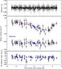 |
Fig. 1 Top: WASP lightcurve of WASP-117 folded on the planetary period. All data are shown in gray, and the phase-folded data, binned into 20 min intervals, are shown in black. Middle: CORALIE (black circles) and HARPS (blue triangles) radial velocities folded on the planetary period together with the best-fitting model (red solid line) and residuals. Bottom: bisector spans of the above RV data. |
2.3. Photometric follow-up
We obtained a total of five high-precision transit lightcurves. Four were observed with the 60 cm TRAPPIST telescope (Gillon et al. 2011; Jehin et al. 2011) using a z’-Gunn filter, and one was obtained with EulerCam at the 1.2 m Euler-Swiss telescope using an r’-Gunn filter. All photometric data were extracted using relative aperture photometry, while carefully selecting optimal extraction apertures and reference stars. More details on EulerCam and the reduction of EulerCam data can be found in Lendl et al. (2012). The resulting lightcurves are shown in Fig. 2.
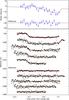 |
Fig. 2 Top: HARPS RVs obtained on 29 Aug. 2013, during a transit of WASP-117b together with the best-fitting model and residuals. Bottom: transit lightcurves observed with (from top to bottom) EulerCam on 29 Aug. 2013, and TRAPPIST on 19 Aug. 2013, 29 Aug. 2013, 08 Sep. 2013, and 28 Sep. 2013 (all UT). The data are offset vertically for clarity. The lightcurves are corrected for their photometric baseline models, the best-fitting transit models are superimposed and the residuals shown below. |
3. Determination of system parameters
3.1. Stellar parameters
The spectral analysis was performed based on the HARPS data. We used the standard pipeline reduction products and co-added them to produce a single spectrum (S/N = 240). We followed the procedures outlined in Doyle et al. (2013) to obtain the stellar parameters given in Table 1. For the vsini determination we have assumed a macroturbulence of 4.28 ± 0.57km s-1 obtained using the asteroseismic-based calibration of Doyle et al. (2014). The lithium abundance suggests an age between 2 and 5 Gyr (Sestito & Randich 2005).
To deduce the stellar mass and estimate the system age, we performed a stellar evolution modeling based on the CLES code (Scuflaire et al. 2008; see Delrez et al. 2014, for details). Using as input the stellar mean density deduced from the global analysis described in Sect. 3.2, and the effective temperature and metallicity from spectroscopy, we obtained a stellar mass of 1.03 ± 0.10 M⊙ and an age of 4.6 ± 2.0 Gyr. This value agrees with the age inferred from the lithium abundance and places WASP-117 on the main sequence. The error budget is dominated by uncertainties affecting the stellar internal physics, especially for the initial helium abundance of WASP-117.
We checked the WASP lightcurves for periodic modulation such as caused by the interplay of stellar activity and rotation using the method described in Maxted et al. (2011). No variations exceeding 95% significance were found above 1.3 mmag. The low activity level of the star is confirmed by a low activity index,  . Using the relation of Mamajek & Hillenbrand (2008) that connects chromospheric activity and stellar rotation, we estimate a stellar rotation period of Prot = 17.1 ± 2.6 days.
3.2. Global analysis
3.2.1. MCMC
We applied a Markov chain Monte Carlo (MCMC) approach to derive the system parameters. Details on MCMCs in astrophysical contexts can be found e.g., in Tegmark et al. (2004). To do so, we carried out a simultaneous analysis of data from the photometric and spectroscopic follow-up observations. We made use of the MCMC implementation described in detail in Gillon et al. (2012), with the fitted (“jump”) parameters listed in Table 2. The transit lightcurves were modeled using the prescription of Mandel & Agol (2002) as well as a quadratic model to describe stellar limb-darkening. A Keplerian together with the prescription of the Rossiter-McLaughlin effect by Giménez (2006) was used for for the RV data. The convective blueshift effect (Shporer & Brown 2011) was not included in the model as its amplitude (~1 m s-1) is well below our 1σ errors. We used the results obtained from the stellar spectral analysis to impose normal prior distributions on the stellar parameters Teff, vsini∗, and [Fe/H], with centers and widths corresponding to the quoted measurements and errors, respectively. Similarly, a normal prior was imposed on the limb-darkening coefficients using values interpolated from the tables by Claret & Bloemen (2011). For the other parameters uniform prior distributions were used.
3.2.2. Photometry
We estimated the correlated (red) noise present in the data via the βr factor (Winn et al. 2008; Gillon et al. 2010), and measured excess white noise, βw, by comparing the calculated error bars to the final lightcurve root-mean square. The photometric error bars were then rescaled by a factor CF = βr × βw for the final analysis. The minimal photometric baseline variation necessary to correct for photometric trends was assumed to be a 2nd-order time polynomial, and an offset at the meridian flip for the TRAPPIST lightcurves. For the TRAPPIST data observed on 28 September 2013, a significant improvement was found by additionally including a 1st-order coordinate dependence.
3.2.3. Radial velocities
To compensate for RV jitter affecting the CORALIE data, we added 10.4 m s-1 quadratically to the CORALIE error bars. The HARPS data did not require any additional jitter. The RV zero points were fitted via minimization at each MCMC step. The inferences drawn from the Rossiter-McLaughlin effect are highly sensitive to any potential RV offsets around the time of transit, as can be caused by stellar activity. Throughout the HARPS RV sequence obtained during the transit of 29 Aug. 2013, we obtained simultaneous photometric observations from EulerCam and TRAPPIST that serve to detect spot-crossing events as well as add information on the precise timing of the transit contact points. No signatures of spot-crossing events are visible in the photometry, in line with the low  activity index observed. To test for any potential RV offset that may still be present, we treated the HARPS data obtained during the night of transit (25 in-, and 3 out-of-transit points) as well as the nights before (1 point) and after (2 points) the transit as independent sequences, allowing for independent RV zero points. The resulting HARPS RV zero points are
 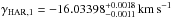 (HARPS, in and near transit), and
 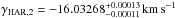 HARPS (other). The two zero points obtained from the HARPS data are in good agreement with each other. Thus we further allow only one RV zero point per instrument, finding
  and γCOR = −16.044910 ± 4.7 × 10⁻⁵ km s-1.
We verified the independence of the Keplerian solution from the in-transit points by carrying out a global analysis excluding the in-transit RVs. The resulting parameters are less than 0.1σ from those found from the analysis of the entire dataset (see Sect. 3.2.4). Similarly, excluding the CORALIE points from the analysis did not produce any significant changes.
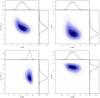 |
Fig. 3 Posterior probability distributions of the parameters β, vsini∗, i∗, and ψ. It is noteworthy that the low projected obliquities β coincide with low values of the stellar inclination i∗ (i.e., a star seen nearly pole-on) and hence a large true orbital obliquity. |
3.2.4. System parameters
The system parameters given in Table 2 were found by running two MCMC chains of 100 000 points each, whose convergence was checked with the Gelman & Rubin test (Gelman & Rubin 1992). As we have knowledge of the parameters e and ω from RVs, we used the transit lightcurves to obtain a measurement of ρ∗ (Kipping 2010). We then inferred the stellar parameters M∗ and R∗ based on the stellar Teff, [Fe/H] and ρ∗ using the calibration of Enoch et al. (2010) that is based on a fit to a sample of main-sequence eclipsing binaries. The stellar parameters obtained from this calibration are in good agreement with those found by stellar evolution modeling.
We find a projected obliquity of β = −44 ± 11 deg that is moderately correlated with the stellar vsini∗, as shown in Fig. 3. The true obliquity, ψ, can be computed if we have information on β, ip, and i∗ (Fabrycky & Winn 2009). Combining our posterior distributions of R∗ and vsini∗ with the estimate of Prot obtained in Sect. 3.1, we calculate  deg. This value, together with the posterior distributions of β and ip, yields deg. As shown in Fig. 3, β and i∗ are correlated such that low values for β correspond to low values of i∗, i.e., near pole-on stellar orientations. WASP-117b is clearly misaligned.
Planetary and stellar parameters for WASP-117 from a global MCMC analysis.
4. Discussion
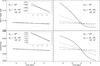 |
Fig. 4 Tidal evolution of the orbital separation (top) and eccentricity (bottom) of WASP-117 b, calculated both forwards and backwards in time. Left: |

With a period of ~10 days, WASP-117b resides in a less densely populated parameter space, well outside the pile-up of giant planets at periods below 5 days. In terms of mean density, this Saturn-mass planet is no outlier with respect to other transiting planets of the same mass range. The orbital eccentricity is well constrained at e = 0.302 ± 0.023. We measure a projected spin-orbit angle of β = −44 ± 11 deg and infer an obliquity of deg.
Owing to its large orbital separation, tidal interactions between star and planet are weaker than for close-in systems. This means that the dampening of eccentricities and orbital decay via tidal interactions is greatly reduced. We integrated Eqs. (1) and (2) of Jackson et al. (2008) both backwards and forwards in time for WASP-117, testing  and
and  values between 105 and 107. We assumed a system age of 4.6 Gyr as well as a main-sequence lifetime of 7.8 Gyr as inferred from the stellar evolution modeling (see Sect. 3.1). The resulting tidal evolutions are shown in Fig. 4. For all tested values, the overall changes in a and e are below 0.004 au and 0.05, respectively, over the systems main-sequence lifetime. Varying substantially from the suggested value of
  (Jackson et al. 2008) allows for some evolution in the orbital eccentricity, but not complete circularization. For the most extreme case studied,
  , an initial eccentricity of 0.67 evolves down to 0.02 over the systems lifetime, together with the orbital separation evolving from 0.135 au to 0.086 au.
Similarly, tidal interactions have been invoked to realign initially misaligned planetary systems (Winn et al. 2010a). To estimate the extent to which this process has impacted the WASP-117 system, we use Eq. (4) of Albrecht et al. (2012) to calculate the efficiency of spin-orbit realignment, assuming a mass of 0.009M∗ in the stellar convective envelope (Pinsonneault et al. 2001). The resulting value τMcz = 4.6 × 10¹² yr, indicates that the orbital obliquity has been essentially unchanged by tidal interactions.
The weak tidal interactions explain why this is one of the few inclined systems amongst stars colder than 6250 K (Winn et al. 2010a). It worth remarking that the other inclined planets orbiting cold stars are also eccentric (e.g., HD 80606b, Hébrard et al. 2008; WASP-8Ab, Queloz et al. 2010; and HAT-P-11b, Winn et al. 2010b). The independence of orbital eccentricity and obliquity from stellar tides make WASP-117b a valuable object for the understanding of planetary migration, and its connection to the properties of close-in planets. It appears that the planet has not undergone an episode of high eccentricity during its migration, as tidal interactions are not strong enough to efficiently circulate a highly eccentric orbit at these large orbital separations. In order to judge the influence of dynamical interactions on the evolution of this system, we encourage follow-up observations aimed at detecting further stellar or planetary companions.
Among the planets outside of the short-period pileup, WASP-117b is one of the most favorable targets for atmospheric characterization, in particular through transmission spectroscopy. This is due to both, a calm, bright (V = 10.15 mag) host star, and an extended planetary atmosphere.
5. Conclusions
The 10-day-period transiting Saturn-mass planet WASP-117b represents the longest-period and one of the lowest-mass planets found by the WASP survey to date. The planetary orbit is eccentric and is inclined with respect to the stellar equator. Tidal interactions between planet and host star are unlikely to have substantially modified either of these parameters over the systems lifetime, making WASP-117b an important piece in the puzzle of understanding the connection between migration and the currently observed orbital properties of close-in planets.
Acknowledgments
WASP-South is hosted by the South African Astronomical Observatory and we are grateful for their ongoing support and assistance. Funding for WASP comes from consortium universities and from the UK’s Science and Technology Facilities Council. TRAPPIST is funded by the Belgian Fund for Scientific Research (Fond National de la Recherche Scientifique, FNRS) under the grant FRFC 2.5.594.09.F, with the participation of the Swiss National Science Fundation (SNF). M. Gillon and E. Jehin are FNRS Research Associates. This work was supported by the European Research Council through the European Union’s Seventh Framework Programme (FP7/2007-2013)/ERC grant agreement number 336480. L. Delrez acknowledges the support of the F.R.I.A. fund of the FNRS. M. Gillon and E. Jehin are FNRS Research Associates. A.H.M.J. Triaud received funding from the Swiss National Science Foundation under grant number P300P2-147773.
References
- Albrecht, S., Winn, J. N., Johnson, J. A., et al. 2012, ApJ, 757, 18 [NASA ADS] [CrossRef] [Google Scholar]
- Asplund, M., Grevesse, N., Sauval, A. J., & Scott, P. 2009, ARA&A, 47, 481 [NASA ADS] [CrossRef] [Google Scholar]
- Bakos, G., Noyes, R. W., Kovács, G., et al. 2004, PASP, 116, 266 [NASA ADS] [CrossRef] [Google Scholar]
- Baranne, A., Queloz, D., Mayor, M., et al. 1996, A&AS, 119, 373 [NASA ADS] [CrossRef] [EDP Sciences] [Google Scholar]
- Baruteau, C., Crida, A., Paardekooper, S.-J., et al. 2014, Protostars and Planets VI, eds. H. Beuther, R. Klessen, C. Dullemond, & Th. Henning (University of Arizona Press), accepted [arXiv:1312.4293] [Google Scholar]
- Batygin, K. 2012, Nature, 491, 418 [NASA ADS] [CrossRef] [PubMed] [Google Scholar]
- Claret, A., & Bloemen, S. 2011, A&A, 529, A75 [NASA ADS] [CrossRef] [EDP Sciences] [Google Scholar]
- Collier Cameron, A., Pollacco, D., Street, R. A., et al. 2006, MNRAS, 373, 799 [NASA ADS] [CrossRef] [Google Scholar]
- Collier Cameron, A., Wilson, D. M., West, R. G., et al. 2007, MNRAS, 380, 1230 [NASA ADS] [CrossRef] [Google Scholar]
- Davies, M. B., Adams, F. C., Armitage, P., et al. 2014, Protostars & Planets VI, eds. H. Beuther, C. Dullemond, Th. Henning, & R. Klessen (University of Arizona Press), accepted [arXiv:1311.6816] [Google Scholar]
- Delrez, L., Van Grootel, V., Anderson, D. R., et al. 2014, A&A, 563, A143 [NASA ADS] [CrossRef] [EDP Sciences] [Google Scholar]
- Doyle, A. P., Smalley, B., Maxted, P. F. L., et al. 2013, MNRAS, 428, 3164 [NASA ADS] [CrossRef] [Google Scholar]
- Doyle, A. P., et al. 2014, MNRAS, submitted [Google Scholar]
- Eggleton, P. P., & Kiseleva-Eggleton, L. 2001, ApJ, 562, 1012 [NASA ADS] [CrossRef] [Google Scholar]
- Enoch, B., Collier Cameron, A., Parley, N. R., & Hebb, L. 2010, A&A, 516, A33 [NASA ADS] [CrossRef] [EDP Sciences] [Google Scholar]
- Fabrycky, D. C., & Winn, J. N. 2009, ApJ, 696, 1230 [NASA ADS] [CrossRef] [Google Scholar]
- Gelman, A., & Rubin, D. 1992, Statist. Sci., 7, 457 [NASA ADS] [CrossRef] [Google Scholar]
- Gillon, M., Lanotte, A. A., Barman, T., et al. 2010, A&A, 511, A3 [NASA ADS] [CrossRef] [EDP Sciences] [Google Scholar]
- Gillon, M., Jehin, E., Magain, P., et al. 2011, Detection and Dynamics of Transiting Exoplanets, St. Michel l’Observatoire, France, eds. F. Bouchy, R. Díaz, & C. Moutou, EPJ Web Conf., 11, 6002 [Google Scholar]
- Gillon, M., Triaud, A. H. M. J., Fortney, J. J., et al. 2012, A&A, 542, A4 [NASA ADS] [CrossRef] [EDP Sciences] [Google Scholar]
- Giménez, A. 2006, ApJ, 650, 408 [NASA ADS] [CrossRef] [Google Scholar]
- Goldreich, P., & Tremaine, S. 1980, ApJ, 241, 425 [NASA ADS] [CrossRef] [MathSciNet] [Google Scholar]
- Gray, D. F. 2008, The Observation and Analysis of Stellar Photospheres (Cambridge: Cambridge University Press) [Google Scholar]
- Hébrard, G., Bouchy, F., Pont, F., et al. 2008, A&A, 488, 763 [NASA ADS] [CrossRef] [EDP Sciences] [Google Scholar]
- Hellier, C., Anderson, D. R., Collier Cameron, A., et al. 2010, ApJ, 723, L60 [NASA ADS] [CrossRef] [Google Scholar]
- Jackson, B., Greenberg, R., & Barnes, R. 2008, ApJ, 678, 1396 [NASA ADS] [CrossRef] [Google Scholar]
- Jehin, E., Gillon, M., Queloz, D., et al. 2011, The Messenger, 145, 2 [NASA ADS] [Google Scholar]
- Kipping, D. M. 2010, MNRAS, 407, 301 [NASA ADS] [CrossRef] [Google Scholar]
- Kozai, Y. 1962, AJ, 67, 591 [Google Scholar]
- Lai, D. 2014, MNRAS, 440, 3532 [NASA ADS] [CrossRef] [Google Scholar]
- Lendl, M., Anderson, D. R., Collier-Cameron, A., et al. 2012, A&A, 544, A72 [NASA ADS] [CrossRef] [EDP Sciences] [Google Scholar]
- Lidov, M. L. 1962, Planet. Space Sci., 9, 719 [NASA ADS] [CrossRef] [Google Scholar]
- Lin, D. N. C., & Papaloizou, J. 1986, ApJ, 309, 846 [NASA ADS] [CrossRef] [Google Scholar]
- Mamajek, E. E., & Hillenbrand, L. A. 2008, ApJ, 687, 1264 [NASA ADS] [CrossRef] [Google Scholar]
- Mandel, K., & Agol, E. 2002, ApJ, 580, L171 [NASA ADS] [CrossRef] [Google Scholar]
- Maxted, P. F. L., Anderson, D. R., Collier Cameron, A., et al. 2011, PASP, 123, 547 [NASA ADS] [CrossRef] [Google Scholar]
- McLaughlin, D. B. 1924, ApJ, 60, 22 [NASA ADS] [CrossRef] [Google Scholar]
- Pepe, F., Mayor, M., Galland, F., et al. 2002, A&A, 388, 632 [NASA ADS] [CrossRef] [EDP Sciences] [Google Scholar]
- Pepper, J., Pogge, R. W., DePoy, D. L., et al. 2007, PASP, 119, 923 [NASA ADS] [CrossRef] [Google Scholar]
- Pinsonneault, M. H., DePoy, D. L., & Coffee, M. 2001, ApJ, 556, L59 [NASA ADS] [CrossRef] [Google Scholar]
- Pollacco, D. L., Skillen, I., Collier Cameron, A., et al. 2006, PASP, 118, 1407 [NASA ADS] [CrossRef] [Google Scholar]
- Queloz, D., Eggenberger, A., Mayor, M., et al. 2000, A&A, 359, L13 [NASA ADS] [Google Scholar]
- Queloz, D., Anderson, D. R., Collier Cameron, A., et al. 2010, A&A, 517, L1 [NASA ADS] [CrossRef] [EDP Sciences] [Google Scholar]
- Rasio, F. A., & Ford, E. B. 1996, Science, 274, 954 [NASA ADS] [CrossRef] [PubMed] [Google Scholar]
- Rossiter, R. A. 1924, ApJ, 60, 15 [NASA ADS] [CrossRef] [Google Scholar]
- Scuflaire, R., Théado, S., Montalbán, J., et al. 2008, Ap&SS, 316, 83 [NASA ADS] [CrossRef] [Google Scholar]
- Seager, S., Richardson, L. J., Hansen, B. M. S., et al. 2005, ApJ, 632, 1122 [NASA ADS] [CrossRef] [Google Scholar]
- Sestito, P., & Randich, S. 2005, A&A, 442, 615 [NASA ADS] [CrossRef] [EDP Sciences] [Google Scholar]
- Shporer, A., & Brown, T. 2011, ApJ, 733, 30 [NASA ADS] [CrossRef] [Google Scholar]
- Tegmark, M., Strauss, M. A., Blanton, M. R., et al. 2004, Phys. Rev. D, 69, 103501 [CrossRef] [Google Scholar]
- Triaud, A. H. M. J. 2011, A&A, 534, L6 [NASA ADS] [CrossRef] [EDP Sciences] [Google Scholar]
- Triaud, A. H. M. J., Collier Cameron, A., Queloz, D., et al. 2010, A&A, 524, A25 [NASA ADS] [CrossRef] [EDP Sciences] [Google Scholar]
- Weidenschilling, S. J., & Marzari, F. 1996, Nature, 384, 619 [NASA ADS] [CrossRef] [PubMed] [Google Scholar]
- Winn, J. N. 2011, in Exoplanet Transits and Occultations, ed. S. Seager (Tucson: University of Arizona Press), 55 [Google Scholar]
- Winn, J. N., Holman, M. J., Torres, G., et al. 2008, ApJ, 683, 1076 [NASA ADS] [CrossRef] [Google Scholar]
- Winn, J. N., Fabrycky, D., Albrecht, S., & Johnson, J. A. 2010a, ApJ, 718, L145 [NASA ADS] [CrossRef] [Google Scholar]
- Winn, J. N., Johnson, J. A., Howard, A. W., et al. 2010b, ApJ, 723, L223 [NASA ADS] [CrossRef] [Google Scholar]
- Wu, Y., & Murray, N. 2003, ApJ, 589, 605 [NASA ADS] [CrossRef] [EDP Sciences] [Google Scholar]
All Tables
All Figures
|
Fig. 1 Top: WASP lightcurve of WASP-117 folded on the planetary period. All data are shown in gray, and the phase-folded data, binned into 20 min intervals, are shown in black. Middle: CORALIE (black circles) and HARPS (blue triangles) radial velocities folded on the planetary period together with the best-fitting model (red solid line) and residuals. Bottom: bisector spans of the above RV data. |
| In the text | |
|
Fig. 2 Top: HARPS RVs obtained on 29 Aug. 2013, during a transit of WASP-117b together with the best-fitting model and residuals. Bottom: transit lightcurves observed with (from top to bottom) EulerCam on 29 Aug. 2013, and TRAPPIST on 19 Aug. 2013, 29 Aug. 2013, 08 Sep. 2013, and 28 Sep. 2013 (all UT). The data are offset vertically for clarity. The lightcurves are corrected for their photometric baseline models, the best-fitting transit models are superimposed and the residuals shown below. |
| In the text | |
|
Fig. 3 Posterior probability distributions of the parameters β, vsini∗, i∗, and ψ. It is noteworthy that the low projected obliquities β coincide with low values of the stellar inclination i∗ (i.e., a star seen nearly pole-on) and hence a large true orbital obliquity. |
| In the text | |
|
Fig. 4 Tidal evolution of the orbital separation (top) and eccentricity (bottom) of WASP-117 b, calculated both forwards and backwards in time. Left: |
| In the text | |
Current usage metrics show cumulative count of Article Views (full-text article views including HTML views, PDF and ePub downloads, according to the available data) and Abstracts Views on Vision4Press platform.
Data correspond to usage on the plateform after 2015. The current usage metrics is available 48-96 hours after online publication and is updated daily on week days.
Initial download of the metrics may take a while.