| Issue |
A&A
Volume 568, August 2014
|
|
|---|---|---|
| Article Number | A11 | |
| Number of page(s) | 14 | |
| Section | Numerical methods and codes | |
| DOI | https://doi.org/10.1051/0004-6361/201423755 | |
| Published online | 05 August 2014 | |
MODA: a new algorithm to compute optical depths in multidimensional hydrodynamic simulations
1 TU Darmstadt, Institut für Kernphysik Theoriezentrum, Schlossgartenstr. 2, 64289 Darmstadt, Germany
e-mail: This email address is being protected from spambots. You need JavaScript enabled to view it.
2 The Oskar Klein Center, Department of Astronomy, AlbaNova, Stockholm University, 106 91 Stockholm, Sweden
3 Department of Physics, University of Basel, Klingelbergst. 82, 4056 Basel, Switzerland
Received: 4 March 2014
Accepted: 5 June 2014
Abstract
Aims. We introduce the multidimensional optical depth algorithm (MODA) for the calculation of optical depths in approximate multidimensional radiative transport schemes, equally applicable to neutrinos and photons. Motivated by (but not limited to) neutrino transport in three-dimensional simulations of core-collapse supernovae and neutron star mergers, our method makes no assumptions about the geometry of the matter distribution, apart from expecting optically transparent boundaries.
Methods. Based on local information about opacities, the algorithm figures out an escape route that tends to minimize the optical depth without assuming any predefined paths for radiation. Its adaptivity makes it suitable for a variety of astrophysical settings with complicated geometry (e.g., core-collapse supernovae, compact binary mergers, tidal disruptions, star formation, etc.). We implement the MODA algorithm into both a Eulerian hydrodynamics code with a fixed, uniform grid and into an SPH code where we use a tree structure that is otherwise used for searching neighbors and calculating gravity.
Results. In a series of numerical experiments, we compare the MODA results with analytically known solutions. We also use snapshots from actual 3D simulations and compare the results of MODA with those obtained with other methods, such as the global and local ray-by-ray method. It turns out that MODA achieves excellent accuracy at a moderate computational cost. In appendix we also discuss implementation details and parallelization strategies.
Key words: methods: numerical / neutrinos / radiative transfer
© ESO, 2014
1. Introduction
Recent years have seen an enormous increase in the physical complexity of multidimensional, astrophysical simulations. This is particularly true for three-dimensional radiation-hydrodynamic simulations as exemplified by recent advances in, say, star formation (e.g., Bate 2012) and core-collapse supernovae (e.g., Janka 2012; Burrows 2013; Ott et al. 2013, and references therein). In the context of radiative transfer problems, the optical depth (τ) is central. When it is calculated from the radiation production site up to the transparent edges of the system, it counts the average number of interactions experienced by a radiation particle before it can finally escape. The optical depth allows the distinction between diffusive (τ ≫ 1), semi-transparent (τ ~ 1), and transparent (τ ≪ 1) regimes. The surface where τ = 2/3 represents the last interaction surface and is often called neutrinosphere in the case of neutrino radiation (or photosphere in the case of photons).
Codes that solve the Boltzmann equations, through either finite difference (e.g., the discrete ordinate method, see Liebendörfer et al. 2004 in 1D; Ott et al. 2008 in 2D; Sumiyoshi & Yamada 2012 in 3D) or spectral methods (e.g., the spherical harmonic method, see Peres et al. 2014), Monte-Carlo codes (e.g., Abdikamalov et al. 2012), and most approximative schemes, such as flux-limited diffusion (e.g., Whitehouse et al. 2005; Swesty & Myra 2009) or M1 schemes (e.g., Shibata & Taniguchi 2011; O’Connor & Ott 2013), do not need to compute τ separately, since it is a physical quantity that results from the algorithm itself. Other codes, such as that of Kuroda et al. (2012), which also employs the M1 closure of the transport equations using a variable Eddington factor, calculate τ assuming that radiation moves along radial paths.
Some approximated radiation transport schemes, like the isotropic diffusion source approximation (Liebendörfer et al. 2009), require the calculation of τ to determine the location of the neutrinospheres. Also, light-bulb methods (e.g., Nordhaus et al. 2010; Hanke et al. 2012; Couch 2013) and ray-tracing methods (e.g., Kotake et al. 2003; Caballero et al. 2009; Surman et al. 2014), in which the neutrino flux intensity in the free-streaming region is computed from the inner-boundary luminosities or by assuming black body emission at the neutrino decoupling surface, often demand the computation of τ, at least where τ ≲ 1.
Codes that treat radiation with leakage schemes (going back to van Riper & Lattimer 1981; Bludman et al. 1982; Cooperstein et al. 1986) need to calculate the optical depth explicitly everywhere inside the computational domain, since it is directly related to the diffusion time scale. In grid-based codes, this is traditionally achieved using either a global or a local ray-by-ray (RbR) approach, while in meshless codes like SPH, one often interpolates the mean free path to a grid, calculates τ just like in the grid-based approach, and then interpolates it back to the SPH particles. The global RbR method employs a number of predefined radial rays, centered on one element of the domain, to calculate the optical depth, and is most effective in geometries with spherical symmetry, such as core-collapse supernovae (CCSNe; Peres et al. 2013; Ott et al. 2013) and isolated (relativistic) stars (Galeazzi et al. 2013). The local RbR method, on the other hand, integrates the optical depth equation along predefined rays starting at each point of the grid. This approach is computationally more expensive, but it is able to handle more complex geometries, and has been used for instance in Newtonian neutron star mergers (Ruffert et al. 1996; Rosswog & Liebendörfer 2003) and neutron star–black hole mergers (Deaton et al. 2013). More recently, neutrino leakage schemes have been adapted to the formalism of general relativity (Sekiguchi 2010; Galeazzi et al. 2013) and used in simulations of neutron star mergers (Sekiguchi et al. 2011).
Our work is motivated by questions related to core-collapse supernovae and neutron star mergers, but our algorithm makes no assumption about the geometry, radiation path, or the astrophysical scenario, and could therefore be readily used in other contexts (e.g., photons in stellar atmospheres).
This paper is organized as follows. Sect. 2 is devoted to a brief review of the concept of optical depth and an outline of our main hypotheses (Sect. 2.1), together with a general description of our new algorithm (Sect. 2.2). In Sect. 3 we describe its implementation in grid-based (Sect. 3.1) and SPH schemes (Sect. 3.2). Section 4.1 presents a number of tests with analytically known solutions, while Sect. 4.2 compares the results of various numerical methods applied to snapshots from grid-based (Sect. 4.2.1) and SPH (Sect. 4.2.2) simulations. Performance and scaling of the multidimensional optical depth algorithm (MODA) are discussed in Sect. 4.3. Finally, our results are summarized in Sect. 5, while technical details about the implementation and the parallelization are presented in , and in .
2. Method
2.1. Definitions and assumptions
The optical depth is a quantitative measure of the interaction between radiation and matter between two points, related on infinitesimal scales to the mean free path λ. Along a path γ connecting two points A and B, the optical depth is defined as  (1)where λ(s) is the local mean free path, and ds is an infinitesimal displacement along the chosen path, γ. Equation (1)already contains the physical interpretation of τ: being related to the inverse mean free path, it counts the average number of interactions between radiation and matter along the path γ.
Even though each radiation particle travels and interacts in its own way and along its own path, for radiation transport problems involving astrophysical (i.e., macroscopic) objects, we are interested in a statistical description of the radiation and in its global behavior (i.e., from the site of production up to the point where radiation can escape). We first notice that from a microscopic point of view1, the production can occur either isotropically (i.e., with equal probabilities in any direction) or anisotropically (for example, in the case of scattering with a non-isotropic phase function and an anisotropic radiation field). On the macroscopic scale, however, the properties of matter influence the behavior of radiation and a traveling particle can lose memory of its emission process: if a radiation particle is emitted toward a region of decreasing mean free path, it will likely interact again with matter, changing its original propagation direction; on the other hand, if it is emitted toward a direction of increasing mean free path, it will probably move away freely from the production site. This simple consideration suggests that, irrespective of the local properties of the emission process, macroscopically radiation moves preferentially toward regions of larger mean free path. Second, the path followed by radiation particles between two points is not therefore necessarily straight: if the two points are separated by a relatively opaque region, radiation emitted in that direction will be likely scattered or absorbed (and, eventually, re-emitted in another direction). Thus, the global, statistical behavior of the radiation moving between those two points will be to bypass that opaque region along a non straight path, characterized by larger mean free paths.
Ultimately, when radiation particles have reached locations where the local mean free path is much larger than the size of the considered domain, they will stream out of the system, practically without further interactions.
The global behavior of the radiation we are interested in requires that, when computing the optical depth according to Eq. (1), a) we can start the path from any point inside the domain; and b) the final point can be any point on the boundary of the computational domain (or possibly in a region transparent to radiation at that wavelength, where boundary conditions also apply). Among all the possible paths connecting A to the boundary, the statistical interpretation suggests to consider the paths that tend to minimize the optical depth (i.e., the paths with the least number of interactions) as the most likely ways for radiation to escape.
Following these prescriptions, we define the optical depth of a point x as  (2)where xe is one point from which radiation can escape freely. The calculation of the optical depth, therefore, implies finding a point xe and a path γ that together tend to minimize the value of τ as given by Eq. (1). In what follows, we present our prescription for finding γ and xe in MODA. Strictly speaking, the solution provided by the algorithm is not necessarily the one that minimizes Eq. (1). However, the search for a global minimum is the guiding principle in constructing, step by step, the path γ toward the boundary of the domain2.
The main algorithm, presented in the next section, is based on the following assumptions:
-
(a)
λ is the only quantity that determines τ, see Eq. (2); the input for our algorithm is therefore a certain spatial distribution λ(x), which can be either analytically known or obtained from a simulation;
-
(b)
λ is a smooth function of position;
-
the boundaries of the computational domain are completely transparent regions, and on large scales λ increases with the distance from the center of the computational domain. However, there can be local variations, and local maxima and minima.
Note that depending on the context one may wish to either compute a spectral or an average (gray) mean free path. Moreover, depending on the radiation–matter interaction processes involved, λ may be either a scattering or an effective total mean free path (see, for example, Raffelt 2001; Shapiro & Teukolsky 1983, Eq. (14.5.57)).
2.2. Algorithm
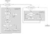 |
Fig. 1 Flow chart of the MODA algorithm. This schematic representation of MODA reveals two distinct steps (the choice of successors and the integration of τ), each of which involves a loop over all grid points (or cells). The algorithm is completely described by this chart, and all specific decisions that are not included in the figure (e.g., how to pick the initial r and how much to successively increase it afterwards) are parametrizations that depend on the underlying implementation (i.e., grid-based or tree-based). |
From the form of Eq. (2)we see that the path that minimizes the optical depth favors regions where the mean free path λ is larger. If λ were a monotonic function of the radial position, ever increasing toward the edges of the computational domain, the algorithm would be trivial: each cell would “pick” its neighbor with the largest λ as the direction of integration, which would guarantee that the optimal solution is achieved.
In practice, however, λ is not always monotonic: non-trivial astrophysical scenarios often contain discontinuities, shocks, clumps of hot dense matter, all of which yield a highly anisotropic and non-homogeneous profile of λ. In such situations, always choosing the local maximum of λ leads to getting “trapped” in regions that are local maxima. On a larger scale, however, the assumption that λ increases toward the edge of the computational domain is still expected to hold. The MODA algorithm makes use of this assumption by searching for sufficiently larger mean free paths, first locally, and if such λ’s are not found then at increasingly larger radii. By parameterizing what “sufficiently larger” means, one is able to obtain a balance between accuracy and speed.
For convenience, since Eq. (2)contains λ in the denominator, we introduce the opacity κ (3)which is the quantity we use in the code instead of λ (since λ → ∞ while κ → 0 toward the edges of the computational domain).
To illustrate the algorithm, let us assume we are interested in the optical depth at a point x. We first define a sphere of radius r1 centered around x, and on its surface  we search for a point z that satisfies
  (4)where fdec ≲ 1 is a parameter3. If such a point is found then the vector
  , with v ≡ z − x, gives the direction of integration. Otherwise, we keep extending our search to spheres of increasing radii ri, with i = 2,3,... until a point z that satisfies Eq. (4)is found. The choice of transparent boundary conditions ensures that this always happens. Once the direction of integration v is found, we simply select – from all the direct neighbors of x – the cell x′ that is in the direction of v, which we call the “successor” of x. Once x′ is known, the search for its own successor can be performed and so on until a point xe on the boundary is reached. The sequence of n intermediate points connecting x and xe, {x(0) ≡ x, x(1) ≡ x′(0), ..., x(i) ≡ x′(i − 1), ..., x(n + 1) ≡ xe}, provides the needed path, γ. Along this path, the optical depth τ(x) is calculated as:
  (5)
(5)
3. Implementation
In the following, we describe a possible implementation of the MODA algorithm on a static grid and in a tree structure. The discussion is accompanied by a flow chart that summarizes all the steps of the algorithm (Fig. 1). In order to keep this description as general as possible, we collect the more technical details in .
In the previous section, we presented the basic concepts focusing on a single starting point. A straightforward implementation would be to successively apply that procedure to each point inside the computational domain. However, this approach is not computationally efficient, since it does not employ a relevant aspect of the problem: given two points, there is a non negligible probability that, depending on the spatial distribution of κ, their two paths toward the edge of the domain merge at a certain point. Given the unambiguous character of the prescription to find the successor, the optical depth of the common part will be the same, and it will be equal to the optical depth of the intersection point. In order to take advantage of this, we divide the implementation of the algorithm into two distinct steps (apart from preliminary operations, such as setting boundary conditions), each applied to the whole domain: 1) finding the relevant distances for the decrease of κ, the integration directions, and the successors; 2) performing the integration. Keeping these steps separate ensures that common paths are not computed multiple times.
3.1. Implementation into a grid code (“grid MODA”)
As an example, we implement the algorithm into the Eulerian, uniform mesh MHD code FISH (Käppeli et al. 2011). The implementation into different types of grid codes (non-uniform and/or non-Cartesian) is straightforward and requires only a moderate amount of changes.
3.1.1. Setting boundary conditions
Setting boundary conditions implies, first of all, providing a predefined value for τ at the edges of the grid:  (6)Safe values for the boundary condition are τboundary ≲ h/λboundary, where h is the local resolution length (cell size) and λboundary is the typical value of the mean free path at the boundary. Since the method requires exploration of neighboring areas, special attention must be given to cells located close to the boundary, for which the spherical surface
  may extend beyond the edges of the domain. There are several possible solutions to this problem; one would be to modify Eq. (4)to search for a direction z that satisfies the opposite condition,
  (7)and then to choose the direction ev by setting v = −(z − x); Another solution would be to set a boundary layer thick enough to prevent one from accessing cells that do not exist.
3.1.2. Finding distances, directions, and successors
We begin searching for points that satisfy Eq. (4)at a distance r1 ~ h, i.e., comparable to the local resolution length h. Instead of calculating the intersection of the grid with the spherical surface  of center x and radius ri (which would become increasingly expensive for high i’s), we sample the surface in a predefined set of m “equidistant” points, Sm(x,ri) = { zj = x + riyj } j = 1,m, where |yj| ≃ 1. Once a point zmin that satisfies Eq. (4)is found inside Sm(x,ri), the radius ri becomes the length scale over which κ decreases down to the chosen limit fdecκ(x).
One could already select vmin = zmin − x as the direction of integration, but this was found to sometimes lead to abrupt discontinuities in the optical depth. To avoid this effect, it is possible to devise a smoothed direction of integration vavg, by using all sampling points inside Sm(x,ri) (or even a subset) and weighting each respective unit direction vector, yj, with a suitable monotonically decreasing function of κ, w(κ):  (8)This average favors the directions where κ is minimum on the spherical surface, but it also takes into account the behavior of κ at the scale of ri, smoothing the evolution of the direction in case of sharp, local variations. In order to avoid compensation effects due to the averaging itself (which would for instance be the case along the axis of symmetry in highly symmetrical configurations, where the average may cancel out the contributions from symmetrical points with the same κdec(x)), we calculate the cosine of the angle between vavg and vmin. If the two directions are too different (i.e., if the cosine is below a threshold, for example cosθlim = 0.9) we reject vavg(x), calculated with Eq. (8), and use vmin(x) instead. The definition of cosθlim sets the maximum allowed discrepancy between the two directions.
Once the direction of integration v (given by either vavg or vmin) has been found, we select the closest cell to x in the direction given by v, from an appropriate set of neighbors, and denote it by x′. It is noteworthy that, although the search for the integration direction vdec(x) is made by “looking ahead” to whatever distance is necessary in order to find an acceptable κ, the integration itself is done in small increments, comparable to the local resolution. The choice of the appropriate set of neighbors, among which x′ has to be searched, has to balance two opposing tendencies: including cells more distant from x increases the angular resolution in searching for x′, but at the same time decreases the accuracy in the path discretization.
In a grid based code determining x′ is relatively simple and efficient, since grid cells have fixed indices based on their geometrical position. We note that all operations involving a cell refer in fact to the geometrical center of the cell. This introduces discretization errors, since most of the times the condition z − x = v cannot be fulfilled exactly (the only exception being paths which traverse entire rows, columns of cells, or which go exactly along diagonals). The impact of this discretization on the resulting path will be shown and explained later on, in Fig. A.1.
Another caveat is that closed circular paths may occur, even though “looking ahead” for the direction decreases the chances of this to happen. Nevertheless, whenever a successor is chosen for a given cell one must check whether it leads to a loop in Eq. (5). If that is the case the next best cell must be picked as a successor. In the tests we have performed, closed loops occurred rarely and usually in presence of very symmetric local extrema of κ. Thus the error introduced by not choosing exactly the direction that tends to minimize the optical depth is usually small and infrequent. The inspection of the integration paths, necessary to discover the presence of loops, has a minor effect on the performance of the algorithm, especially compared with the more demanding searches of the distances and of the directions.
3.1.3. Performing the integration
Once the direction of integration has been found throughout the entire computational domain, each cell falls into one of these two categories: either it is a boundary point, in which case τ is already known there, or it is a point inside the computational domain, in which case one knows in what direction radiation moves away from it. The actual integration takes the form of a loop through all the cells: those for which τ is known are simply skipped, while for the others the integration path is reconstructed by following the list of successors, until arriving to a cell with known τ. The integral in Eq. (5)then becomes a sum of partial Δτ’s,  (9)where κ(i,i − 1) is an average between κ(x(i)) and κ(x(i − 1)), x(0) = x, and τ(x(l)) is the first already-computed value of the optical depth along the path γ (or, in case γ does not overlap with an already-computed path, x(l) = xe).
3.2. Implementation using a tree structure (“tree MODA”)
Our goal is to implement the MODA algorithm into an SPH code (for recent reviews of this method see, e.g., Monaghan 2005 and Rosswog 2009). Most SPH codes make use of hierarchical structures (trees) to search for particle neighbors and calculate gravitational forces. In what follows, we will describe the implementation of MODA into a recently developed recursive coordinate bisection (RCB) tree (Gafton & Rosswog 2011). The implementation strategy, however, is not restricted to this type of tree and can straightforwardly be adapted to other tree types such as octree (Barnes & Hut 1986) or other binary trees (Benz et al. 1990).
The RCB tree is not built down to the last particle, but down to small groups of adjacent particles that are always aggregated into what we call “lowest-level cells” (or ll-cells), also found in the “tree literature” as “leaves” (Oxley & Woolfson 2003; Springel 2005; Gaburov et al. 2010; Hubber et al. 2011; Clark et al. 2012) or as “buckets” (Dikaiakos & Stadel 1996; Stadel 2001; Wadsley et al. 2004). Since the average number of particles per ll-cell (typically ~12) is much smaller than the average neighbor number (~100), the size of any ll-cell will always be smaller than the smoothing length of its particles. Since the smoothing length is the typical length scale over which physical quantities are resolved in SPH, one does not expect the mean free path to exhibit large variations within any one ll-cell. It is therefore unnecessary to calculate the optical depth τ for each individual particle, and one expects the same results by computing it per ll-cell. This idea has also been followed by Oxley & Woolfson (2003), whose radiative transfer scheme for SPH uses tree leaves as the radiating and absorbing elements, and by Stamatellos & Whitworth (2005), who use cells whose linear size is comparable to the local smoothing length.
In principle, the algorithm for a tree follows the steps presented in Sect. 3.1: successively larger radii are used for searching for a sufficiently larger mean free path, and once the correct direction is found, the successor of the current cell is chosen as the closest cell in the respective direction. In our tree-adapted version of the MODA algorithm, “grid cell” translates into “ll-cell”. Since cells located at a certain radius cannot be identified by simply operating on cell indices, as in the case of grid-based codes, we rely on the tree walk infrastructure of the RCB tree (Gafton & Rosswog 2011, Sect. 2.2) to return a list of ll-cells located within a certain spherical shell of radius r and parametrized width dr. Furthermore, once the direction of integration is known, one cannot use a predetermined list of directions, described by known angles, to quickly find the closest cell in the necessary direction. One must instead compute the angle between the directions to the surrounding cells (which can in principle be pre-computed upon building the tree) and the desired direction of integration, and then pick the best (i.e., the largest cosine). On the other hand, once the successors are known for all ll-cells, the integration step is virtually identical to that performed by grid MODA.
4. Tests, applications, and performance
In this section, we apply both versions of MODA to two types of three dimensional configurations: first, to cases with analytically known inputs and, when possible, solutions (cases 1–3), and, second, to practical astrophysical applications (cases A–D). The former (Sect. 4.1) are validation tests for some simple cases where λ and κ are analytic functions of the Cartesian coordinates, while the latter (Sect. 4.2) are based on snapshots from real astrophysical simulations. The solutions compared in each case were obtained with some of the following methods: (a) analytic solution, if available; (b) grid MODA; (c) tree MODA; (d) local RbR method; (e) global RbR method. In Table 1 we summarize the cases we have explored and the available solutions.
Summary of all the configurations we have analyzed and the solutions available for each of them.
In the local RbR method, we integrate κ along a set of predefined straight paths (rays) from each point of the grid, and choose the optical depth at that point to be the minimum amongst these integrals. To obtain a local directional resolution comparable with the one provided by MODA, we choose 98 directions, passing by the centers of the neighboring cells satisfying Eq. (A.1). In the global RbR method, we interpolate κ from the Cartesian mesh to a spherical one, calculate the local τ by integrating κ along the radial path, and interpolate τ back on the Cartesian mesh. The spherical mesh is characterized by 30 polar and 60 azimuth angles.
4.1. Analytic tests
The simplest possible tests for MODA involve analytic, spherically symmetric distributions κ(r), see Eq. (3). For such tests, the direction of integration is known (it can only be the outward radial direction, by symmetry), and the optical depth τ can therefore be computed analytically. These are also the most insightful tests since the error can be computed for each individual cell or particle, and the reason for each deviation can usually be pin-pointed and understood, allowing us to acknowledge the inherent limitations of MODA. Tests 1 and 2 below are based on two such configurations, while test 3 involves a more complex (non-spherically symmetric, though still analytic) spatial configuration.
For grid MODA, the computational domain is an equally-spaced Cartesian grid of 6003 cells, with each cell having unitary width.
For tree MODA, we represent the κ profile by ~105 (in tests 1 and 2) or 2 × 10⁶ (in test 3) particles. As a conservative precaution we use ~1 particle per ll-cell. Where this is not possible due to the tessellation algorithm, we prescribe the λ of an ll-cell to be the average of the λ’s of all its particles.
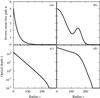 |
Fig. 2 Analytic κ and τ for tests 1 and 2. This plot shows the spherically symmetric initial conditions κ(r) and optimal results τ(r) for the first two analytic tests: a) monotonic κ(r) as given by Eq. (10); b) non-monotonic κ(r) as given by Eq. (12); c)τ(r) as given by Eq. (11); d)τ(r) as given by Eq. (13). |
Test 1: monotonic, spherically symmetric.
For the first and simplest test we define a monotonically decreasing spherically symmetric inverse mean free path  (10)where r is the radial distance from the center of the computational domain, which is (0,0,0) in our Cartesian coordinate system. For our tests we use κ0 = 5, d0 = 30, which leads to the distribution shown in Fig. 2a, with the solution being the analytic function
 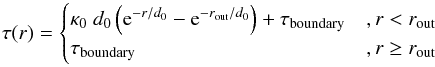 (11)as shown in Fig. 2c. The boundary conditions are defined by the cutoff radius rout = 249 and the optical depth of the transparent regime, τ(r>rout) = 10-2. We use a parameter fdec = 0.8, see Eq. (4).
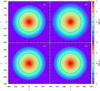 |
Fig. 3 Results of test 1. Logarithm of optical depth τ for the first (monotonic, spherically symmetric) analytic test, as obtained with four methods: a) analytic solution (see Eq. (11)and Fig. 2c); b) tree MODA; c) grid MODA; d) local RbR. Contour lines correspond to log τ = −1,0,1. Qualitatively, the plots are in agreement. The small deviations from spherical symmetry appearing at the edges in the tree MODA plot are largely due to interpolation to the grid used for plotting. |
In Fig. 3 we present the resulting optical depth calculated with different methods. The fact that contours of τ are concentric circles shows that all algorithms accurately reproduce the original spherical symmetry of the input data. While spherical symmetry is directly encoded in the analytic solution and in the global RbR method, Fig. 3a, it is less obvious for MODA, where no symmetry and no predefined path is assumed.
The larger error of tree MODA (especially near the boundary rout, where τ is very low) is both due to the lower resolution compared to the grid code (6003 vs. 105) and due to the interpolation on the regular grid used for plotting. In astrophysical simulations, the former issue can be considerably attenuated by sampling the fluid well enough, i.e., by making sure that all particles have a sufficiently large number of neighbors and that the smoothing lengths are well below the relevant physical scales.
Test 2: non-monotonic, spherically symmetric.
The second test is also spherically symmetric, but has a non-monotonic feature (a local maximum) halfway through the computational domain, which simulates non-monotonic profiles that often appear in real simulations, as discussed in Sect. 2.2 and as will be clearly seen in the astrophysical tests (Sect. 4.2). This distribution is defined as the superposition of a Gaussian centered in the origin and an off-centered Gaussian, 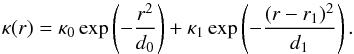 (12)For our tests we use the parameters κ0 = 5, κ1=2, d0 = 8000, d1 = 1000, r1 = 150 in order to get the distribution shown in Fig. 2b. The integration of Eq. (12)can be performed analytically, with the result being
 ![Mathematical equation: \begin{equation} \tau(r)=\begin{cases} \begin{array}{ll} \frac{\sqrt{\pi}}{2}&\left\{ \sqrt{d_0}\invlam_0 \left[-\erf\left(\frac{r}{\sqrt{d_0}}\right)+\erf\left(\frac{\rout}{\sqrt{d_0}}\right)\right]\right.\\ &\phantom{\left\{\right.}+ \sqrt{d_1}\invlam_1 \left.\left[-\erf\left(\frac{r-r_1}{\sqrt{d_1}}\right)+\erf\left(\frac{\rout-r_1}{\sqrt{d_1}}\right)\right]\right\} \\ & \; + \; \tau_{\rm boundary},\quad r<\rout \end{array}&\\ \tau_{\rm boundary},\quad r\geq\rout& \end{cases} \label{eq:tau analytic 2} \end{equation}](/articles/aa/full_html/2014/08/aa23755-14/aa23755-14-eq105.png) (13)where erf(x) is the Gauss error function. This leads to the profile τ(r) shown in Fig. 2d. The same boundary conditions apply as before, i.e., rout = 249, τ(r>rout) = 10-2, and fdec = 0.8.
(13)where erf(x) is the Gauss error function. This leads to the profile τ(r) shown in Fig. 2d. The same boundary conditions apply as before, i.e., rout = 249, τ(r>rout) = 10-2, and fdec = 0.8.
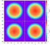 |
Fig. 4 Results of test 2. Logarithm of optical depth τ for the second (non-monotonic, spherically symmetric) analytic test, as obtained with four methods: a) analytic solution (see Eq. (13)and Fig. 2d); b) tree MODA; c) grid MODA; d) local RbR. Contour lines correspond to log τ = −1,0,1. |
The results are presented in Fig. 4 and are consistent with those in the previous section, with all three methods yielding excellent results, even though tree MODA is slightly worse near the boundaries, where the SPH resolution is poorest.
Test 3: asymmetric.
For the third model we define a superposition of two off-centered, elliptical Gaussian distributions ![Mathematical equation: \begin{eqnarray} \invlam(x_1,x_2,x_3)&=&\sum_{n\,=\,1,2}\invlam_n \exp\left[-\left(\frac{x_1-\tilde x_{1,n}}{s_{1,n}}\right)^2\right.\nonumber\\ &&\left.-\left(\frac{x_2-\tilde x_{2,n}}{s_{2,n}}\right)^2 -\left(\frac{x_3-\tilde x_{3,n}}{s_{3,n}}\right)^2 \right],\label{eq:sigma analytic 3} \end{eqnarray}](/articles/aa/full_html/2014/08/aa23755-14/aa23755-14-eq107.png) (14)with κ1 = 120, κ2 = 80, s1,1 = 35, s2,1 = 30, s3,1 = 25, s1,2 = 45, s2,2 = 15, s3,2 = 30,
(14)with κ1 = 120, κ2 = 80, s1,1 = 35, s2,1 = 30, s3,1 = 25, s1,2 = 45, s2,2 = 15, s3,2 = 30,  , and
, and  . The same boundary conditions apply, i.e., rout = 249 and τ(r>rout) = 10-2. This time we use fdec = 0.5, since the more complicated geometry requires more accuracy and larger decreases in the distance determination.
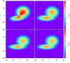 |
Fig. 5 Results of test 3 (z = 0 cross-section). Logarithm of optical depth τ for the third (non-spherically symmetric) analytic test, as obtained with four methods: a) global RbR; b) tree MODA; c) grid MODA; d) local RbR. The plots represent a cut through the z = 0 plane. Contour lines correspond to log τ = −1,0,1. |
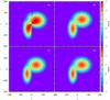 |
Fig. 6 Results of test 3 (x = 0 cross-section). Logarithm of optical depth τ for the third (non-monotonic, spherically symmetric) analytic test, as obtained with four methods: a) global RbR; b) tree MODA; c) grid MODA; d) local RbR. The plots represent a cut through the x = 0 plane. Contour lines correspond to log τ = −1,0,1. |
Two sets of results are shown, corresponding to cross-sections of the z = 0 plane (Fig. 5) and of the x = 0 plane (Fig. 6). The integration of Eq. (14)is not straightforward to perform analytically, since the direction of integration is not radial, but highly dependent on the position. For this reason, we use the results obtained with the local RbR method as reference, Figs. 5d and 6d. In contrast to the previous cases, the global RbR method (Figs. 5a and 6a), shows inaccuracies and artifacts due to the lack of spherical symmetry of κ. On the other hand, the other tests are qualitatively consistent, and show remarkable agreement and similar resolution.
Two important considerations, common to all the tests we have performed, have to be pointed out. First, the optical depth is a physical quantity that can usually span a wide range of values (five orders of magnitude in this example); therefore, large relative errors in a limited number of zones (particularly near the edges, where τ is essentially zero) do not imply a noticeable effect on the overall calculation of τ. Second, MODA provides a comparable result at a considerably lower computational cost than the local RbR method (see Sect. 4.3).
4.2. Astrophysical applications
We now turn to real astrophysical scenarios, and we choose snapshots of multidimensional simulations with highly asymmetrical and non-isotropic configurations, that span orders of magnitude in density.
In order to apply our algorithm, we consider thermodynamical conditions extracted from 3D simulations and, based on them, we calculate the physical λ for electron neutrinos with a specific energy (chosen to be 54 MeV). Once the λ and hence the κ distribution is obtained, all subsequent steps are identical to those from the analytic tests.
4.2.1. Grid MODA
Case A: core-collapse supernova
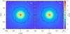 |
Fig. 7 Results of case A. Logarithm of optical depth τ for the astrophysical case A, as obtained with two methods: a) grid MODA; b) global RbR. Contour lines correspond to log τ = −1,0,1. |
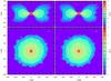 |
Fig. 8 Results of case B. Logarithm of optical depth τ for the astrophysical case B, as obtained with two methods: a) and c) grid MODA; b) and d) local RbR. Top (bottom) panels refer to y = 0 (z = 0) cross-sections. Contour lines correspond to log τ = −1,0,1. |
In the first application, we take a 2D Cartesian slice of data (density, temperature, and electron fraction), from a 3D core collapse supernova simulation performed with the ELEPHANT code (Whitehouse & Liebendörfer 2008), with a spatial resolution of 2 km. Considering that the system is, to a first approximation, spherically symmetric, we calculate the electron neutrino optical depth using grid MODA and the global RbR method (with the polar angle discretized by 64 angular bins). Both results are shown in Fig. 7. We find similar results with both methods: inside a radius of about 60 km (which includes the proto-neutron star and the inner part of the shocked material), the optical depth contours are spherically symmetric, as expected. Above that radius, matter is convective and multidimensional effects come into play. The contour lines start to show multidimensional features, which are related to non-homogeneous features in density, temperature, and electron fraction. The main difference between both methods is the spatial resolution of the results. While the RbR approach decreases its resolution moving outwards, the new algorithm maintains a constant resolution. As a result, the outer optical depth contours are smoother than those found by the global RbR method.
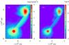 |
Fig. 9 Results of case C. a) Logarithm of density ρ and b) logarithm of optical depth τ for the astrophysical application C. The density profile is taken directly from the simulation output, while τ is computed with tree MODA. The SPH resolution is N ~ 6 × 10⁵ particles. The plot shows a z = 0 cross section. Contour lines correspond to log τ = −2.4, − 0.3,1. |
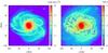 |
Fig. 10 Results of case D. a) Logarithm of density ρ and b) logarithm of optical depth τ for the astrophysical application D. The density profile is taken directly from the simulation output, while τ is computed with tree MODA. The SPH resolution is N ~ 8 × 10⁶ particles. The plot shows a z = 0 cross-section, and only the inner 200 km of the disc (≳1000 km) are shown. Contour lines correspond to log τ = 1,2,3. |
Case B: neutron star merger remnant
As a second application case we take the matter distribution (density, temperature, and electron fraction) from the remnant of a double neutron star merger simulation (Price & Rosswog 2006), performed with the SPH code MAGMA (Rosswog & Price 2007), and map the particles onto a 3D Cartesian, equidistant grid with spatial resolution of 2 km. The calculation of the optical depth is performed with grid MODA and the results are shown in Fig. 8a and c, along with the results of a local RbR method in Fig. 8b and d. The two plots are in good agreement, though fine-structure differences do appear. We suspect that these differences are mainly due to the fact that our method is based on a purely local exploration of the suitable radiation path, and does not invoke any special global symmetry or predefined direction. In this sense, our 3D method provides an optical depth calculation that is more general and automatically adapts to the geometry of the matter distribution. The high resolution, three dimensional local RbR method is, also in this case, prohibitively expensive from a computational point of view, and the resolution shown in this test is never achieved with this method in actual hydrodynamic calculations.
4.2.2. Tree MODA
The input for the tree MODA tests was produced with a version of the MAGMA code (Rosswog & Price 2007). From the densities and electron fractions of the SPH particles we computed the mean free paths for E = 54 MeV neutrinos.
We present the results of tree MODA alone for two reasons. First, we do not have another particle-based code that computes optical depths for SPH simulations. Second, due to the intrinsic resolution adaptivity that characterizes SPH codes, it would not be straightforward to compare those results with the ones obtained by grid MODA, after having remapped the SPH matter distribution on a uniform grid.
Case C: white dwarf collision
The first astrophysical application of tree MODA uses a snapshot from an off-center collision between a 0.6 M⊙ and a 0.9 M⊙ white dwarf (Rosswog et al. 2009) from a simulation with ~6 × 10⁵ SPH particles. The density profile and the resulting optical depth are shown in Fig. 9 for a z = 0 cross section. At this stage, the stars had a first close encounter and are now moving toward their apocenter separation before they fall back toward each other again. Some debris shed in the collision is aligned in the form of a temporary “matter bridge” between the two stars. Note that the secondary (near y = 6 × 109 cm) is heavily spun up by tidal torques. Since the E = 54 MeV neutrino mean free path is comparable to the size of the white dwarfs, one could expect the maximum optical depth (at the center of the star) to be around 1. The results of our calculations are in agreement with that: the contour lines of τ for the heavier star are concentric circles and have a maximum value of ~1; the lighter star has a much smaller optical depth, and the tidal bridge is essentially transparent and comparable in τ to the debris halos surrounding the two stars.
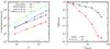 |
Fig. 11 Performance comparison between MODA and the RbR algorithm. Left: computational time as a function of the effective number of cells N, obtained with both the serial codes and their OpenMP versions using 8 threads. Right: computational efficiency as a function of the number of OpenMP threads. For these parallelization tests, the dimension of the computational domain is fixed at N = 4003. |
Case D: neutron star collision
The second application for tree MODA is a snapshot from a high resolution (~8 × 10⁶ particles) simulation of a collision of two neutron stars of masses 1.4 M⊙ and 1.3 M⊙ (Rosswog et al. 2013). The density profile and the resulting optical depth are shown in Fig. 10 for a z = 0 cross section. The snapshot provides a late-stage picture of the encounter, when, after several close passages a pulsing and rapidly rotating central remnant, surrounded by shocked debris from several mass shedding episodes has formed. The entire structure has a radius of ≳500 km, but we show just the inner 100 km, where most of the mass is concentrated, and the debris contains a number of fine structures from the mass shedding and subsequent shocks. This is a highly non-trivial, non-isotropic, and asymmetric problem. Still, the resulting optical depth profile found by MODA accurately portrays the complex debris structure.
4.3. Performance
In this section, we compare the performance of grid MODA and of the local RbR method, the two grid-based methods that are able to handle complex matter distributions without specific symmetries. We focus on three-dimensional simulations, where the computational effort is higher and, consequently, the impact of the optical depth calculation cost is larger. In order to compare the scalings with the grid size we employ a computational domain of size N = N1/3 × N1/3 × N1/3, and compare both the serial and the OpenMP versions with Nthreads = 8. As test case we use analytic test 1 (see Sect. 4.1). The values of N1/3 range from 200 to 600 for all cases and the results are presented in Fig. 11a. In addition of being a more general method that automatically adapts to the geometry of the matter distribution, MODA is usually more than one order of magnitude faster than the local RbR method (in the serial as well as the parallelized versions), and exhibits better scaling with increasing N (tMODA ~ N1.75 while tRbR ~ N2.31).
In the case of MODA, we notice that most of the computational time (~70%) is spent to find, for each point of the domain, the relevant distance where κ decreases enough to satisfy Eq. (4).
Most loops appearing in MODA have been parallelized from the beginning using OpenMP constructs. Its scaling with the number of OpenMP threads, shown in Fig. 11b by the so-called efficiency η = T1/(pTp) (where T1 is the serial computational time and Tp is the computational time using p threads) is much better than the efficiency of a RbR algorithm.
5. Conclusions
In this paper we presented a new, efficient algorithm for the calculation of optical depths τ from any given profile of the mean free path λ. There are no restrictions related to the symmetry or the configuration of the computational domain. All that is needed is that λ be globally increasing toward the edges of the domain, which is normally a fair assumption. The algorithm was implemented both in a grid-based and a tree-based code, and proved to be suitable for both Eulerian and Lagrangian methods. The three-dimensional tests we presented, starting with analytic, spherically-symmetric configurations, and ending with highly anisotropic and heavily shocked configurations, proved that the algorithm provides excellent accuracy in multidimensional calculations, while being less computationally expensive than more traditional RbR methods.
By macro-/microscopic we mean large/small in comparison to the local mean free path λ.
We note that a slight overestimation of the minimum optical depth is not necessarily incorrect, even considering the assumptions of our method. The (theoretical) minimum is the smallest value that τ could possibly take (anything below that is nonphysical), but (slightly) larger values are of course possible and perhaps to be expected in nature.
Typical values of fdec that we have tested (see Sect. 4 for more details) lie in the interval 0.1 − 0.8. Larger values, closer to unity, can be less effective in avoiding local extrema, while smaller values require more computational effort, and are prone to push the decreasing length scale search too early toward the edge of the computational domain, introducing boundary conditions effects. In any case, we recommend a careful examination of κ(x), and its typical spatial and temporal variations, in order to choose an adequate value for fdec.
Acknowledgments
A.P. was supported by the Helmholtz-University Investigator grant No. VH-NG-825; he also thanks the Stockholm University for its hospitality in June 2013, and the University of Basel for its hospitality in January 2014, during the final stages of the development of MODA. E.G. thanks the University of Basel for its hospitality during the summer of 2011, when the work on the SPH version of MODA was initiated. E.G. and S.R. acknowledge the use of computational resources provided by the Höchstleistungsrechenzentrum Nord (HLRN), and the use of SPLASH developed by D. Price to visualize SPH simulations. R.C. and M.L. acknowledge the support from the HP2C Supernova project and the ERC grant FISH. A.P., R.C. and M.L. are thankful for the use of computational resources provided by the Swiss Supercomputing Center (CSCS), under allocation grants s412 and s414.
References
- Abdikamalov, E., Burrows, A., Ott, C. D., et al. 2012, ApJ, 755, 111 [NASA ADS] [CrossRef] [Google Scholar]
- Barnes, J., & Hut, P. 1986, Nature, 324, 446 [NASA ADS] [CrossRef] [Google Scholar]
- Bate, M. R. 2012, MNRAS, 419, 3115 [NASA ADS] [CrossRef] [Google Scholar]
- Benz, W., Cameron, A. G. W., Press, W. H., & Bowers, R. L. 1990, ApJ, 348, 647 [NASA ADS] [CrossRef] [Google Scholar]
- Bludman, S. A., Lichtenstadt, I., & Hayden, G. 1982, ApJ, 261, 661 [NASA ADS] [CrossRef] [Google Scholar]
- Burrows, A. 2013, Rev. Mod. Phys., 85, 245 [NASA ADS] [CrossRef] [Google Scholar]
- Caballero, O. L., McLaughlin, G. C., & Surman, R. 2009, Phys. Rev. D, 80, 123004 [NASA ADS] [CrossRef] [Google Scholar]
- Clark, P. C., Glover, S. C. O., & Klessen, R. S. 2012, MNRAS, 420, 745 [NASA ADS] [CrossRef] [Google Scholar]
- Cooperstein, J., van den Horn, L. J., & Baron, E. A. 1986, ApJ, 309, 653 [NASA ADS] [CrossRef] [Google Scholar]
- Couch, S. M. 2013, ApJ, 775, 35 [NASA ADS] [CrossRef] [Google Scholar]
- Deaton, M. B., Duez, M. D., Foucart, F., et al. 2013, ApJ, 776, 47 [NASA ADS] [CrossRef] [Google Scholar]
- Dikaiakos, M., & Stadel, J. 1996, in In Proc. of the 10th ACM International Conference on Supercomputing. ACM, 94 [Google Scholar]
- Gaburov, E., Bédorf, J., & Portegies Zwart, S. 2010, Procedia Computer Science, 1, 1119 [CrossRef] [Google Scholar]
- Gafton, E., & Rosswog, S. 2011, MNRAS, 418, 770 [NASA ADS] [CrossRef] [Google Scholar]
- Galeazzi, F., Kastaun, W., Rezzolla, L., & Font, J. A. 2013, Phys. Rev. D, 88, 4009 [Google Scholar]
- Goldberg, D. 1991, ACM Comput. Surv., 23, 5 [CrossRef] [Google Scholar]
- Hanke, F., Marek, A., Müller, B., & Janka, H.-T. 2012, ApJ, 755, 138 [Google Scholar]
- Hubber, D. A., Batty, C. P., McLeod, A., & Whitworth, A. P. 2011, A&A, 529, A27 [NASA ADS] [CrossRef] [EDP Sciences] [Google Scholar]
- Janka, H.-T. 2012, Ann. Rev. Nucl. Part. Sci., 62, 407 [Google Scholar]
- Käppeli, R., Whitehouse, S. C., Scheidegger, S., Pen, U.-L., & Liebendörfer, M. 2011, ApJS, 195, 20 [NASA ADS] [CrossRef] [Google Scholar]
- Knuth, D. E. 1973, The art of computer programming (Reading, MA: Addison-Wesley) [Google Scholar]
- Kotake, K., Yamada, S., & Sato, K. 2003, ApJ, 595, 304 [NASA ADS] [CrossRef] [Google Scholar]
- Kuroda, T., Kotake, K., & Takiwaki, T. 2012, ApJ, 755, 11 [NASA ADS] [CrossRef] [Google Scholar]
- Liebendörfer, M., Messer, O. E. B., Mezzacappa, A., et al. 2004, ApJS, 150, 263 [NASA ADS] [CrossRef] [Google Scholar]
- Liebendörfer, M., Whitehouse, S. C., & Fischer, T. 2009, ApJ, 698, 1174 [NASA ADS] [CrossRef] [Google Scholar]
- Monaghan, J. J. 2005, Rep. Prog. Phys., 68, 1703 [Google Scholar]
- Nordhaus, J., Burrows, A., Almgren, A., & Bell, J. 2010, ApJ, 720, 694 [NASA ADS] [CrossRef] [Google Scholar]
- O’Connor, E., & Ott, C. D. 2013, ApJ, 762, 126 [NASA ADS] [CrossRef] [Google Scholar]
- Ott, C. D., Burrows, A., Dessart, L., & Livne, E. 2008, ApJ, 685, 1069 [NASA ADS] [CrossRef] [Google Scholar]
- Ott, C. D., Abdikamalov, E., Mösta, P., et al. 2013, ApJ, 768, 115 [NASA ADS] [CrossRef] [Google Scholar]
- Oxley, S., & Woolfson, M. M. 2003, MNRAS, 343, 900 [NASA ADS] [CrossRef] [Google Scholar]
- Pawlik, A. H., & Schaye, J. 2008, MNRAS, 389, 651 [NASA ADS] [CrossRef] [Google Scholar]
- Peres, B., Oertel, M., & Novak, J. 2013, Phys. Rev. D, 87, 043006 [NASA ADS] [CrossRef] [Google Scholar]
- Peres, B., Penner, A. J., Novak, J., & Bonazzola, S. 2014, Class. Quant. Grav., 31, 045012 [NASA ADS] [CrossRef] [Google Scholar]
- Press, W. H., Teukolsky, S., Vetterling, W., & Flannery, B. 1992, Numerical recipes in Fortran. The art of scientific computing, 2nd edn. (Cambridge University Press) [Google Scholar]
- Price, D. J., & Rosswog, S. 2006, Science, 312, 719 [NASA ADS] [CrossRef] [PubMed] [Google Scholar]
- Raffelt, G. G. 2001, ApJ, 561, 890 [NASA ADS] [CrossRef] [Google Scholar]
- Rosswog, S. 2009, New Astron. Rev., 53, 78 [NASA ADS] [CrossRef] [Google Scholar]
- Rosswog, S., & Liebendörfer, M. 2003, MNRAS, 342, 673 [NASA ADS] [CrossRef] [Google Scholar]
- Rosswog, S., & Price, D. 2007, MNRAS, 379, 915 [NASA ADS] [CrossRef] [Google Scholar]
- Rosswog, S., Kasen, D., Guillochon, J., & Ramirez-Ruiz, E. 2009, ApJ, 705, L128 [NASA ADS] [CrossRef] [Google Scholar]
- Rosswog, S., Piran, T., & Nakar, E. 2013, MNRAS, 430, 2585 [NASA ADS] [CrossRef] [Google Scholar]
- Ruffert, M., Janka, H.-T., & Schaefer, G. 1996, A&A, 311, 532 [NASA ADS] [Google Scholar]
- Sekiguchi, Y. 2010, Class. Quant. Grav., 27, 4107 [CrossRef] [Google Scholar]
- Sekiguchi, Y., Kiuchi, K., Kyutoku, K., & Shibata, M. 2011, Phys. Rev. Lett., 107, 051102 [NASA ADS] [CrossRef] [PubMed] [Google Scholar]
- Shapiro, S. L. & Teukolsky, S. A. 1983, Black holes, white dwarfs, and neutron stars (New York, NY: Wiley) [Google Scholar]
- Shibata, M., & Taniguchi, K. 2011, Liv. Rev. Rel., 14, 6 [Google Scholar]
- Springel, V. 2005, MNRAS, 364, 1105 [NASA ADS] [CrossRef] [Google Scholar]
- Stadel, J. G. 2001, Ph.D. Thesis, University of Washington, USA [Google Scholar]
- Stamatellos, D., & Whitworth, A. P. 2005, A&A, 439, 153 [NASA ADS] [CrossRef] [EDP Sciences] [Google Scholar]
- Sumiyoshi, K., & Yamada, S. 2012, ApJS, 199, 17 [NASA ADS] [CrossRef] [Google Scholar]
- Surman, R., Caballero, O. L., McLaughlin, G. C., Just, O., & Janka, H.-T. 2014, J. Phys. G Nuclear Physics, 41, 4006 [Google Scholar]
- Swesty, F. D., & Myra, E. S. 2009, ApJS, 181, 1 [NASA ADS] [CrossRef] [Google Scholar]
- Thomson, J. 1904, Philosophical Magazine Series 6, 7, 237 [CrossRef] [Google Scholar]
- van Riper, K. A., & Lattimer, J. M. 1981, ApJ, 249, 270 [NASA ADS] [CrossRef] [Google Scholar]
- Wadsley, J. W., Stadel, J., & Quinn, T. 2004, New Astron., 9, 137 [NASA ADS] [CrossRef] [Google Scholar]
- Wales, D. J., & Ulker, S. 2006, Phys. Rev. B, 74, 212101 [NASA ADS] [CrossRef] [Google Scholar]
- Whitehouse, S., & Liebendörfer, M. 2008, in Proc. 10th Symp., Nuclei in the Cosmos X, available at http://pos.sissa.it/cgi-bin/reader/conf-cgi?confid=53 [Google Scholar]
- Whitehouse, S. C., Bate, M. R., & Monaghan, J. J. 2005, MNRAS, 364, 1367 [NASA ADS] [CrossRef] [Google Scholar]
Appendix A: Technical implementation details
In this appendix, we provide more technical details about our actual implementation of MODA in a static Cartesian grid (Sect. A.1) and in a tree-code (Sect. A.2).
Appendix A.1: Grid code
Setting boundary conditions. Concerning the setting of the boundary conditions, in our grid implementation of MODA the definition of a thick boundary layer has been chosen, since it is easier to implement and faster to execute. However it has the small disadvantage of reducing the size of the useful computational domain: in the boundary layer, the optical depth takes by definition a constant, predefined value τboundary, according to Eq. (6). This may not be a problem since the choice of a constant is based on the (generally valid) assumption that the area near the edge of the computational domain is completely transparent to radiation (i.e., λboundary ≫ h). The width of the layer is assumed to be 8% of the linear size of the computational box. The standard value used in MODA for the boundary optical depth is τboundary = 10-2.
Finding the distances, the directions, and the successors. The investigation of the inverse mean free path on a sphere of radius ri and center x is the first step in the search for x′, the local successor point of x. As described in Sect. 3.1.2, this is done by sampling the spherical surface with a set of m equidistant points, Sm(x,ri) = { x + riyj } j = 1,m, where |yi| ≃ 1. While in two dimensions these would simply be m points on a circle separated by angles of 2π/m radians; in three dimensions, we choose { yj } j = 1,m as the solutions of the Thomson problem (Thomson 1904; Wales & Ulker 2006) on a unitary sphere. In all our tests, we adopted m = 64.
The function w(κ), used in Eq. (8)to devise a smoothed direction of integration is w(κ) = 1 /κ. The maximum allowed angular distance between vmin and vavg is set by cosθlim = 0.9. After the determination of the ideal integration direction v, the successor point has to be found out of a suitable set of neighbors. For this set, we consider all cells z(i′,j′,k′) around x(i,j,k) that satisfy  (A.1)(here i, j, and k, eventually primed, are integers representing the Cartesian coordinate of the cell within the grid). In the cases where two cells have their centers aligned with x, we choose the one closest to x. In total, the number of neighbors is 98.
Since angular operations are easier in spherical coordinates, one begins by extracting the direction (θ,ϕ) of the vector v. Then one loops through the neighboring cells. In this loop, one discards all the cells that are too “far” from the direction ϕ, which is not expensive to check: since one already knows the relative position of the surrounding cells, one can easily store and retrieve the pre-computed spherical components of z − x. Once the list of cells is culled, the spherical distance between all normalized direction vectors (z − x)/ | z − x | and the normalized direction  is computed, and the closest cell in the direction of v is chosen.
Performing the integration. In the calculation of Eq. (9), λ(i,i − 1) is computed as the arithmetic average between κ(x(i)) and κ(x(i − 1)). For a uniform grid, this corresponds to the application of the trapezoidal rule for the calculation of Δτ.
Appendix A.2: SPH code
We illustrate the steps of the tree MODA algorithm in Fig. A.1, which uses a very basic, two-dimensional, spherically symmetric computational domain with very low resolution, and presents a typical path found by tree MODA. All steps discussed below can be traced on the figure.
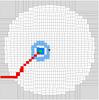 |
Fig. A.1 Example of a path found by tree MODA. This simple test for a two-dimensional Sobol distribution (see Press et al. 1992, Sect. 7.7) with 104 particles (1024 ll-cells) and a spherically symmetric, monotonic mean free path profile (see Sect. 4.1) reveals most of the inner workings and the problems of the algorithm. See text in for details. |
Setting the boundary condition. The boundary condition for the optical depth, described by Eq. (6), is assigned in a similar way as for the grid-based code, although tree MODA does not need such a broad boundary (since only cells that are literally touching the edges of the computational domain, i.e., the gray cells in Fig. A.1, need to be assigned the boundary conditions).
Empty ll-cells. Due to the tessellation provided by the tree code, empty cells may appear anywhere in the computational domain. For spatially-balanced trees, which create cells according to a prescription independent of the particle distribution, it is obvious why empty cells appear (see Fig. 1 in Barnes & Hut 1986). In density-balanced trees, on the other hand, they appear in low-density regions and are compensated for by “over-populated” ll-cells in dense regions, since the RCB tree enforces by construction an “average” number of particles per ll-cell. In general, the lower the “average” number of particles per ll-cell and the less homogeneous the system is, the higher the chances are of empty ll-cells being produced. As the RCB tree is built proactively, all empty cells are effectively compressed into zero volume, and then ignored in all tree walks and during the integration of τ, because they do not contain useful information (i.e., particles).
Finding the correct direction of integration. A tree walk –similar to the neighbor search tree walk – performed for each ll-cell A (in the figure, a fiducial cell shown in green) returns a list of ll-cells that are closer to A than a certain value dx (the dark blue cells). By setting dx to an infinitesimally small value we obtain the simplest possible test, in which the cells must touch (dx should not be exactly zero due to the imprecise nature of floating point arithmetic, see, e.g., Knuth 1973, Sect. 4.2 of the second volume; or Goldberg 1991). In practice we allow dx to be a little larger, a fraction of the typical size of the cell, since the tessellation may, in rare cases, produce cells which are extremely close to each other but do not quite touch.
Once the list of neighboring cells is obtained, one loops through them and checks whether Eq. (4)holds for any of them. If it does, the one with the largest mean free path is picked as successor. Otherwise, the search radius is extended and another tree walk is performed, which returns a list of ll-cells (in the figure, the light blue cells) whose centers of mass fall within a spherical shell of radius r2 and width dr (marked by the two black circles). The operation continues until a suitable cell is found. Since all boundary cells count as “suitable”, this will always happen eventually.
We note that the search radius and its increments are not fixed throughout the computational domain, like in grid MODA, but are functions of the local smoothing length. This is necessary because of the adaptive resolution of SPH: in dense regions smoothing lengths are small and we only need to slightly extend the search radius in order to sample more ll-cells – and implicitly particles, while in less dense regions smoothing lengths are large and we need to look further away in order to sample the same number of cells.
The algorithm returns a (correct) straight path for as long as the cells are aligned just like in a grid, but it cannot do so once the underlying cell structure becomes irregular. When that happens, the path deviates from the expected radial path and the (minimum) optical depth is over-estimated.
A more subtle error of the algorithm (which can be only alleviated by increasing the resolution) can be observed as follows. If one draws the radial line from the center of the computational domain (black cross) to our fiducial green cell, one sees that the path found by tree MODA is not in fact along the radial direction (which in this case would be close to horizontal). This is a discretization problem caused by the low resolution of the mesh of ll-cells. One notices that there are eight direct neighbors at r1. Because the profile of λ is radial, MODA will choose the lower-left corner cell (since its center of mass is further away than that of, e.g., the cell directly to the left, it also has larger λ), even though this may not lead to the correct analytic solution. The same problem appears at radius r2: because of the discretization, the spherical shell is not uniformly filled with cells, and there are cells whose center of mass “just doesn’t make it” into the shell (e.g., immediately to the right of the domain center). MODA will select the best possible solution from the list of cells and most of the times it will provide a very reasonable approximation, but one has to keep this in mind as being an important source of error.
Finding the closest cell in the correct direction. If a cell with a large enough mean free path has been found amongst the very first neighbors (this can happen if the value of f in Eq. (4)is very small, which in practice is a bad idea since it may lead to getting trapped in regions of local maxima, as explained in Sect. 2.2) then that cell is chosen as a successor.
Otherwise, it means that we have a direction of integration (given by the coordinates of the cell found in the previous step) and need to find the closest ll-cell in the respective direction. Achieving directed transport has long been a problem in SPH: radiation propagates along straight lines, while a typical SPH particle distribution is highly irregular: if one wants to find the closest cell in a given direction, the least complicated approach is to compute the direction vector to each neighboring cell, and then the cosine of the angle between that vector and the desired direction of integration. The cell which gives the largest cosine will be the best approximation to the desired direction.
If one implements tree MODA at the level of particles instead of ll-cells, an interesting alternative is the concept of virtual SPH particles (Pawlik & Schaye 2008): instead of searching for an actual particle that is only approximately in the desired direction of integration, a virtual particle is created exactly in the direction where it is needed, at a distance comparable with the local resolution length, allowing the path to proceed in exactly the desired direction. Implementing this into the current code is not straightforward: the path cannot stop at the newly-introduced virtual particle, so after its creation one needs to find its successor as well; this means that one would need to maintain two separate lists, a list of ll-cells and a list of virtual particles, etc.
Performing the integration. Once the direction of integration has been found throughout the entire computational domain the integration is performed in a very similar manner to the grid MODA, by means of a recursive subroutine. For each ll-cell, the successor is known and can fall in one of two categories: either its optical depth τ is not yet known, in which case it is recursively computed, or it is known, in which case Eq. (9)is evaluated with l = 1, i.e., by just computing the increase in the optical depth when moving between the two cells, and then adding it to the already-computed optical depth of the successor.
Appendix B: Parallelization
Parallelization of grid MODA. Most loops appearing in MODA have been parallelized from the beginning using OpenMP constructs. However, the integration of MODA into a complex MPI code such as FISH (Käppeli et al. 2011) requires special attention. By far the most challenging issue is that calculating the optical depth τ (and here we include both the determination of an integration path, and the evaluation of the integral itself), requires information from the entire computational domain. This is problematic in an MPI environment, where the information about the computational domain is distributed between multiple nodes, each with its own separate memory. The repeated exchange of necessary information between all nodes would be highly expensive, and a MODA-like algorithm that only needs to exchange information about the boundary zones between neighboring subdomains has not yet been devised. On the other hand, the calculation of τ only depends on the mean free path, which is a local quantity that can be computed by each MPI node separately; moreover, the calculation of τ is efficient and has been OpenMP parallelized. The natural solution is then to set aside one node (i.e., the “MODA node”) for the sole purpose of the optical depth calculation. This node receives a list of mean free paths from all processors, calculates the optical depth using the MODA algorithm, and then sends back the list of optical depths to each respective processor.
Initial experiments have shown that the calculation of the optical depth for one energy bin in core collapse supernova simulations with FISH takes of the order of one MHD time step. Since ~20 energy bins are typically used, and both the effective and the total optical depth (see Sect. 2.1) need to be calculated, a few possibilities exist to balance the time spent in these two parts of the code:
-
(a)
The optical depth can be assumed to not change significantlyafter one MHD time step, therefore τ can be evaluated once every few time steps; for example, if computing τ for each of the 20 energy bins takes ~one MHD time step, then the optical depth will effectively be calculated once every 20 time steps, which depending on the simulation may be sufficient.
-
(b)
Optical depths are dependent on the neutrino energy, however we can assume that their paths do not change significantly between two neighboring energy bins. It may therefore suffice to only calculate the integration path (which is the most expensive part of MODA) for three representative energy values (“low”, “medium”, “high”), and then for each of the 20 energy bins to choose which of the three paths is more appropriate and perform the integration along it – using the correct spectral mean free paths.
-
(c)
One can also use multiple MODA nodes, e.g., three nodes, one for each energy regime described in (b), or two nodes, one for the effective and one for the total optical depth, etc.
Parallelization of tree MODA. The four parts of the tree MODA algorithm described in are – at this stage – parallelized with OpenMP. The tree walks that find the successor of each cell greatly resemble those performed by the SPH neighbor search and the gravity calculations, in that they are performed independently for each ll-cell. This makes the algorithm ideal for parallelization with OpenMP. The integration of the optical depth is also easy to parallelize, although it may happen that, if several threads work at the same time on cells that have partially overlapping integration paths, the calculation for the common part will be done multiple times.
All Tables
Summary of all the configurations we have analyzed and the solutions available for each of them.
All Figures
|
Fig. 1 Flow chart of the MODA algorithm. This schematic representation of MODA reveals two distinct steps (the choice of successors and the integration of τ), each of which involves a loop over all grid points (or cells). The algorithm is completely described by this chart, and all specific decisions that are not included in the figure (e.g., how to pick the initial r and how much to successively increase it afterwards) are parametrizations that depend on the underlying implementation (i.e., grid-based or tree-based). |
| In the text | |
|
Fig. 2 Analytic κ and τ for tests 1 and 2. This plot shows the spherically symmetric initial conditions κ(r) and optimal results τ(r) for the first two analytic tests: a) monotonic κ(r) as given by Eq. (10); b) non-monotonic κ(r) as given by Eq. (12); c)τ(r) as given by Eq. (11); d)τ(r) as given by Eq. (13). |
| In the text | |
|
Fig. 3 Results of test 1. Logarithm of optical depth τ for the first (monotonic, spherically symmetric) analytic test, as obtained with four methods: a) analytic solution (see Eq. (11)and Fig. 2c); b) tree MODA; c) grid MODA; d) local RbR. Contour lines correspond to log τ = −1,0,1. Qualitatively, the plots are in agreement. The small deviations from spherical symmetry appearing at the edges in the tree MODA plot are largely due to interpolation to the grid used for plotting. |
| In the text | |
|
Fig. 4 Results of test 2. Logarithm of optical depth τ for the second (non-monotonic, spherically symmetric) analytic test, as obtained with four methods: a) analytic solution (see Eq. (13)and Fig. 2d); b) tree MODA; c) grid MODA; d) local RbR. Contour lines correspond to log τ = −1,0,1. |
| In the text | |
|
Fig. 5 Results of test 3 (z = 0 cross-section). Logarithm of optical depth τ for the third (non-spherically symmetric) analytic test, as obtained with four methods: a) global RbR; b) tree MODA; c) grid MODA; d) local RbR. The plots represent a cut through the z = 0 plane. Contour lines correspond to log τ = −1,0,1. |
| In the text | |
|
Fig. 6 Results of test 3 (x = 0 cross-section). Logarithm of optical depth τ for the third (non-monotonic, spherically symmetric) analytic test, as obtained with four methods: a) global RbR; b) tree MODA; c) grid MODA; d) local RbR. The plots represent a cut through the x = 0 plane. Contour lines correspond to log τ = −1,0,1. |
| In the text | |
|
Fig. 7 Results of case A. Logarithm of optical depth τ for the astrophysical case A, as obtained with two methods: a) grid MODA; b) global RbR. Contour lines correspond to log τ = −1,0,1. |
| In the text | |
|
Fig. 8 Results of case B. Logarithm of optical depth τ for the astrophysical case B, as obtained with two methods: a) and c) grid MODA; b) and d) local RbR. Top (bottom) panels refer to y = 0 (z = 0) cross-sections. Contour lines correspond to log τ = −1,0,1. |
| In the text | |
|
Fig. 9 Results of case C. a) Logarithm of density ρ and b) logarithm of optical depth τ for the astrophysical application C. The density profile is taken directly from the simulation output, while τ is computed with tree MODA. The SPH resolution is N ~ 6 × 10⁵ particles. The plot shows a z = 0 cross section. Contour lines correspond to log τ = −2.4, − 0.3,1. |
| In the text | |
|
Fig. 10 Results of case D. a) Logarithm of density ρ and b) logarithm of optical depth τ for the astrophysical application D. The density profile is taken directly from the simulation output, while τ is computed with tree MODA. The SPH resolution is N ~ 8 × 10⁶ particles. The plot shows a z = 0 cross-section, and only the inner 200 km of the disc (≳1000 km) are shown. Contour lines correspond to log τ = 1,2,3. |
| In the text | |
|
Fig. 11 Performance comparison between MODA and the RbR algorithm. Left: computational time as a function of the effective number of cells N, obtained with both the serial codes and their OpenMP versions using 8 threads. Right: computational efficiency as a function of the number of OpenMP threads. For these parallelization tests, the dimension of the computational domain is fixed at N = 4003. |
| In the text | |
|
Fig. A.1 Example of a path found by tree MODA. This simple test for a two-dimensional Sobol distribution (see Press et al. 1992, Sect. 7.7) with 104 particles (1024 ll-cells) and a spherically symmetric, monotonic mean free path profile (see Sect. 4.1) reveals most of the inner workings and the problems of the algorithm. See text in for details. |
| In the text | |
Current usage metrics show cumulative count of Article Views (full-text article views including HTML views, PDF and ePub downloads, according to the available data) and Abstracts Views on Vision4Press platform.
Data correspond to usage on the plateform after 2015. The current usage metrics is available 48-96 hours after online publication and is updated daily on week days.
Initial download of the metrics may take a while.