| Issue |
A&A
Volume 568, August 2014
|
|
|---|---|---|
| Article Number | A35 | |
| Number of page(s) | 7 | |
| Section | Planets and planetary systems | |
| DOI | https://doi.org/10.1051/0004-6361/201423723 | |
| Published online | 11 August 2014 | |
Impact of micro-telluric lines on precise radial velocities and its correction⋆
1 Centro de Astrofísica da Universidade do Porto, rua das Estrelas, 4150-762 Porto, Portugal
e-mail: This email address is being protected from spambots. You need JavaScript enabled to view it.
2 Departamento de Física e Astronomia, Faculdade de Ciências, Universidade do Porto, Portugal
3 Université Versailles Saint-Quentin; Sorbonne Université, UPMC Univ. Paris 06; CNRS/INSU, LATMOS-IPSL, 11 boulevard d’Alembert, 78280 Guyancourt, France
4 Observatoire Astronomique de l’Université de Genève, 51 Ch. des Maillettes, Sauverny, 1290 Versoix, Suisse
Received: 27 February 2014
Accepted: 10 June 2014
Abstract
Context. In the near future, new instruments such as ESPRESSO will arrive, allowing us to reach a precision in radial velocity measurements on the order of 10 cm s-1. At this level of precision, several noise sources that until now have been outweighed by photon noise will start to contribute significantly to the error budget. The telluric lines that are not neglected by the masks for the radial velocity computation, here called micro-telluric lines, are one such noise source.
Aims. In this work we investigate the impact of micro-telluric lines in the radial velocities calculations. We also investigate how to correct the effect of these atmospheric lines on radial velocities.
Methods. The work presented here follows two parallel lines. First, we calculated the impact of the micro-telluric lines by multiplying a synthetic solar-like stellar spectrum by synthetic atmospheric spectra and evaluated the effect created by the presence of the telluric lines. Then, we divided HARPS spectra by synthetic atmospheric spectra to correct for its presence on real data and calculated the radial velocity on the corrected spectra. When doing so, one considers two atmospheric models for the synthetic atmospheric spectra: the LBLRTM and TAPAS.
Results. We find that the micro-telluric lines can induce an impact on the radial velocity calculation that can already be close to the current precision achieved with HARPS, and so its effect should not be neglected, especially for future instruments such as ESPRESSO. Moreover, we find that the micro-telluric lines’ impact depends on factors, such as the radial velocity of the star, airmass, relative humidity, and the barycentric Earth radial velocity projected along the line of sight at the time of the observation.
Key words: atmospheric effects / techniques: radial velocities / planets and satellites: detection
Appendix A is available in electronic form at http://www.aanda.org
© ESO, 2014
1. Introduction
Since the discovery in 1995 of the first planet orbiting another star than the Sun by Mayor & Queloz (1995), more than 1000 exoplanets have been discovered1. From these, more than half were detected using the radial velocity (RV) technique. The RV method consists in measuring the Doppler shifts of the stellar spectra caused by the back and forth movement of the star around the center of mass of the planetary system. The current ace in exoplanet discovery through the RV method is HARPS, a fiber-fed, cross-dispersed échelle spectrograph installed on the 3.6-m telescope at La Silla Observatory, which routinely achieves a precision better than 1 m s-1 (Mayor et al. 2003) and down to 50 − 60 m s-1 (Dumusque et al. 2012). The RV calculation from HARPS observations is done using the cross-correlation function (CCF) technique (Baranne et al. 1996), with the wavelength being calibrated using a Th-Ar lamp, which imprints emission lines over the wavelength domain of the spectrograph.
Several other techniques have been demonstrated. More recently, Anglada-Escudé & Butler (2012) developed a new algorithm implemented in a piece of software called HARPS-TERRA to derive RVs from HARPS data using least square matching of each observed spectrum to a high signal-to-noise ratio (S/N) template derived from the same observation. Besides the emission lamp technique, it is also common to use a gas absorption cell as wavelength calibrator. A common absorption gas is iodine (I2). Several spectrographs are equipped with this technology (e.g., the HIRES spectrograph at the Keck telescope). Because the iodine absorption cell can be positioned directly in front of the slit, the spectrum entering the slit is, in fact, the product of the gas cell spectrum and the stellar one. This method allows a RV precion of 1 − 2 m s-1 (Marcy & Butler 1992; Butler et al. 1996).
This level of precision is still not sufficient to find an Earth-like planet on a one-year orbit around a Sun-like star; for reference, the impact of Earth in the solar RV is of only ~9 cm s-1. Therefore, a new generation of high-precision spectrographs is currently being planned with the objective of detecting Earth-mass planets; among these, ESPRESSO stands out. It aims for a precision of ten cm s-1 (Pepe et al. 2010) and has, as one of the main science goals, detection of an earth-mass planet in the habitable zone of a Sun-like star. An increase in precision (and accuracy) implies a more detailed characterization of systematics and, in particular, the need to be more careful with contamination sources. As an example, the reader can look at the work of Cunha et al. (2013) which presents a study of the impact by companions within the fiber in the RV calculation, where the contaminants are the secondary star of a binary system, a back/foreground star, and even just the moonlight.
One other possible source of contamination is the Earth’s atmosphere itself. Like all high-resolution spectrographs, HARPS is a ground-based spectrograph, and so, atmospheric spectra is imprinted on top of the stellar one. To minimize the effect of this contamination on RVs computation, 3 of the 72 HARPS spectral orders, the ones in which the deeper telluric lines are present, are neglected in the RV computation (Mayor et al. 2003). Moreover, in other spectral orders with deep telluric lines and/or strong blended lines, stellar masks used in the CCF take only a very few stellar lines into consideration (Baranne et al. 1996; Pepe et al. 2002). But as the S/N of the spectra increases and the calibration methods are improved, the relative impact of shallow, not-neglected telluric lines, here designated as micro-telluric lines, will become stronger. Therefore, it becomes urgent to explore how to study the impact of these telluric lines of smaller depth and how to correct their effect on the RV calculation.
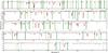 |
Fig. 1 Normalized synthetic atmospheric spectra obtained with TAPAS (top black line) and LBLRTM (bottom dashed black line). The thick vertical green lines represent the position, for a velocity V = 0, of stellar lines in the G2 stellar mask used by HARPS, and its intensity the weight in the CCF. |
The pursuit for the best method of correcting stellar spectra from atmospheric lines is not a recent matter. One possible way of doing it is to use standard stars, for which spectral features are well known, to determine the atmospheric spectrum (see, e.g., Vacca et al. 2003). Using simulations, Bailey et al. (2007) show that, for infrared observations, using an Earth atmospheric transmission spectrum modeled with spectral mapping atmospheric radiative transfer model (SMART) leads to better correction of the telluric lines than using the “division by a standard star” technique. Following the Bailey et al. (2007) work, Seifahrt et al. (2010) developed a method of calibrating the wavelength of CRIRES spectrograph and correcting its observations from telluric lines by modeling the Earth atmospheric transmission spectra with the line-by-line radiative transfer model (LBLRTM). Also, Cotton et al. (2014) used the division by modeled telluric spectra to remove of telluric features from Jupiter and Titan’s infrared spectra, just to cite a few examples from an extensive list.
The present paper follows the method that resorts to theoretical atmospheric transmission spectra to remove telluric features from stellar spectra. To achieve that, the atmospheric models, LBLRTM and the Transmissions Atmosphériques Personnalisées Pour l’AStronomie (TAPAS), which are described in Sect. 2, are used. In Sect. 3 we present a study of the impact of the micro-telluric lines by adding an atmospheric spectrum to a synthetic Sun-like stellar spectrum, and in Sect. 4 this effect is corrected by removing the atmospheric spectra from HARPS spectra. We finish with a discussion about our work and present our conclusions in Sect. 5.
2. Atmospheric spectra with LBLRTM and TAPAS
In this section we describe the two atmospheric models used in this work: LBLRTM and TAPAS, which are not independent. The LBLRTM is an accurate model derived from the fast atmospheric signature code (FASCODE; Clough et al. 1981, 1992), which uses the HITRAN database (HIgh-resolution TRANsmission molecular absorption database) as the basis for the line parameters. This is a very versatile model, which besides the pre-defined models, also accepts a user-supplied atmospheric profile. In this work, for the LBLRTM, we used atmospheric data from the Air Resources Laboratory (ARL) – Real-time Environmental Applications and Display sYstem (READY) Archived Meteorology2. Because ARL-READY only provides data up to 26 km of altitude, for higher atmospheric layers we used the MIPAS model atmospheres (2001) for the mid-latitude, night-time3. If one wants to have absolute control over the input parameters for the atmospheric spectra, LBLRTM is undoubtedly the model to use. The drawback in using LBLRTM is the lack of user friendliness in the input method and the somewhat cryptic, highly technical user instructions. Therefore, in this work we also tested a more user friendly model: TAPAS.
TAPAS is a free online service that simulates atmospheric transmission4. TAPAS makes use of the ETHER (Atmospheric Chemistry Data Centre) facility to interpolate within the European Centre for Medium-Range Weather Forecasts (ECMWF) pressure, temperature, and constituent profile at the location of the observing site and within six hours of the date of the observations, and it computes the atmospheric transmittance from the top of the atmosphere down to the observatory, based on the HITRAN and the LBLTRM code. TAPAS is much more user friendly than LBLRTM, although users have less control, having a much smaller number of input parameters. For more details the user is referred to Bertaux et al. (2014).
Figure 1 shows the spectra obtained with both models, using identical physical conditions as input. The two spectra overlap significantly but show a few differences (red shadow area between lines). One can also see in Fig. 1 that some telluric lines fall within or close to the mask lines, and they are taken into account in the RV calculation.
To compare the ability of the two models to reproduce the atmospheric transmission, a spectrum of a spectral type O5 star was corrected from the Earth’s atmospheric absorption using both models. A HD 46223 HARPS spectrum, taken during the program ID 185.D-0056(L), with a S/N of 220 at the center of the spectral order number 50 (which corresponds to a wavelength of 4372.8 Å). The choice of an O5 star was motivated by the low number of spectral lines. Figure 2 shows the normalized stellar spectra before correction, and after correction with LBLRTM and with TAPAS. We also computed the standard deviations σO5/LBLRTM and σO5/TAPAS in a part of the spectra without stellar lines, but with telluric spectral lines (6474.6 Å <λ< 6518.3 Å), as a measurement of the scattering of the corrected spectra. We obtained σ values of 0.0078 and of 0.0081, respectively. Both models correct well the atmosphere, since both their standard deviations (σO5/LBLRTM and σO5/TAPAS) are of the same order of magnitude, differing by a small amount (~3.7%). In this work we have chosen to use the TAPAS method because it is easier.
3. Synthetic stellar spectra test
Before correcting HARPS spectra from telluric lines absorption, we first calculated the impact of the micro-telluric lines using synthetic stellar spectra of a solar star, i.e., the difference between the RV obtained when using the stellar spectra with and without the atmosphere. The synthetic spectrum was built by extracting the spectral lines using VALD (Viena Atomic Line Database, Piskunov et al. 1995; Ryabchikova et al. 1997; Kupka et al. 1999, 2000), and then computing the spectrum using the running option synth of MOOG (Sneden 1973). This spectra was multiplied by TAPAS atmospheric spectra for one night with H2O vertical column of 14.52 kg m-3. The water vapor content is relevant since the micro-telluric lines are partially H2O, and thus the lines’ depth varies with the water vapor content. Moreover, the lines’ depth in the atmospheric spectra increases as the airmass increases. Therefore, we obtained TAPAS spectra for different values of the zenith angle (and so different values of airmass), using the same time of observation as input. In doing so we only consider zenithal angles of up to 60°, i.e., for airmass values below 2.
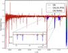 |
Fig. 2 Normalized spectrum of the spectral type O5 HD 46223 star (blue); normalized spectrum of the spectral type O5 star HD 46223 divided by the atmospheric spectrum obtained with LBLRTM (green); normalized spectrum of the spectral type O5 star HD 46223 divided by the atmospheric spectrum obtained with TAPAS (red). |
For each simulated atmospheric spectra we then changed the RV of the star by shifting the stellar spectra from RV = − 100 km s-1 to RV = 100 km s-1 in steps of 1 km s-1. The RV of each spectrum, with and without atmosphere, was calculated by cross-correlating it with a template (Baranne et al. 1996; Pepe et al. 2002). We then calculated the impact of the atmosphere as the difference between the RV of the original spectra (RVo) and the RV of the modified spectra (RVm): 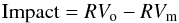 (1)In the case of the synthetic stellar spectra, the original spectra will be the one without atmosphere, and the modified one the one with atmosphere. The results are presented in Fig. 3, where one can see that the impact of the atmosphere will depend on the airmass and on the RV of the star, as expected. The impact of the different models scales with airmass.
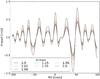 |
Fig. 3 Impact of the atmosphere in the RV calculation for airmass values between 1 and 2. The inner line represents the airmass = 1 and the outer the airmass =2. |
When one compares the maximum impact for the different values of airmass (Fig. 4), one can see that the micro-telluric lines can introduce an RV variation that is large enough to mimic or hide a planet. This is especially relevant when searching for small planets using observations on different nights with a large relative difference in the H2O vertical column, or when the same star is observed several times in one night with large H2O vertical column variation.
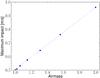 |
Fig. 4 Maximum impact for the different airmass values. |
4. Correcting HARPS spectra from micro-telluric lines
4.1. Data
In his section we investigate the impact of the atmospheric micro-telluric lines on real spectra obtained with HARPS. To do so, we used 18 Sco time series of data obtained on the night of 2012-05-19 under the program ID 183.D-0729(B), allowing therefore the study of the impact of the airmass in the RVs along the night. The S/N at the center of the spectral order number 50 (S/N50) of the 18 Sco observations varies between 124 and 212.4, and the H2O vertical column predicted by TAPAS varies between 3.83 and 4.51 kg m-3.
To complement the analysis of the 18 Sco data, we also used spectra of three other stars, ranging in spectral type from G to M – Tau Ceti (G8), HD 85512 (K5), and Gl436 (M1). As in our previous work on the impact of stellar companions on precise RVs (Cunha et al. 2013), where these stars were also used, we chose these stars because they were the ones for which we could find HARPS spectra for their spectral type with the highest S/N. We used spectra with S/N50 ranging between 30 for the M star, and 439 for the G star. The values of S/N of the used spectra can be found in Table A.1, along with the airmass and the Program ID for each observation.
4.2. Method
To determine the impact of the atmosphere in the RV calculation using HARPS spectra, we divided the HARPS stellar spectra by the normalized TAPAS synthetic atmospheric spectra. The TAPAS spectra used for each stellar spectra correction from the atmosphere is obtained using, as input parameters: the Observatory (ESO La Silla Chile); the exact date and hour of the observation; the spectral range in wavenumber units (14 450 − 26 550cm-1); the instrumental function as Gaussian; the ARLETTY atmospheric model, which is an ETHER atmospheric profile computed by using the nearest in time of the ECMWF meteorologic field observation; a resolution power of 115 000 (HARPS’ resolution); a sampling ratio, i. e., the number of points on which the convolved transmission will be sampled for each interval of FWHM, of 10; and the Zenithal angle of the star.
All the remaining preferences of the TAPAS request form were the default ones. To convert the wavenumber (WVNR) to the air wavelength (AIR) used in HARPS spectra, we first converted into vacuum wavelength (VAC): ![Mathematical equation: \begin{equation} \label{eq:wnr-vac} {\it WVNR}\left[\mathrm{cm}^{-1}\right]=\frac{10^8}{{\it VAC}\left[\AA \right]}\cdot \end{equation}](/articles/aa/full_html/2014/08/aa23723-14/aa23723-14-eq25.png) (2)Then we used the IAU standard conversion from AIR to VAC as given by Morton (1991)
(2)Then we used the IAU standard conversion from AIR to VAC as given by Morton (1991)![Mathematical equation: \begin{equation} \label{eq:air-vac} {\it AIR} \left[\AA\right]=\frac{{\it VAC}\left[\AA\right]}{(1.0 + 2.735182\times10^{-4}+\frac{131.4182}{{\it VAC}\left[\AA\right]^2}+\frac{2.76249\,\times\,10^8}{{\it VAC}\left[\AA\right]^4})}\cdot \end{equation}](/articles/aa/full_html/2014/08/aa23723-14/aa23723-14-eq26.png) (3)Because the atmospheric spectra wavelength grid is different than HARPS wavelength grid, we interpolated the atmospheric wavelength grid to the HARPS grid. On top of that, we shifted the atmospheric spectra of ± 1500 m s-1 in steps of 1 m s-1, we divided the normalized stellar spectra by each shifted atmospheric spectra, and we calculate which shifted spectra minimizes the difference between the stellar spectrum before and after atmospheric correction by minimizing the χ2. This will be the atmospheric spectra that best corrects for the atmosphere, since more telluric lines of the atmospheric spectrum will coincide with the telluric lines present in the stellar spectrum.
(3)Because the atmospheric spectra wavelength grid is different than HARPS wavelength grid, we interpolated the atmospheric wavelength grid to the HARPS grid. On top of that, we shifted the atmospheric spectra of ± 1500 m s-1 in steps of 1 m s-1, we divided the normalized stellar spectra by each shifted atmospheric spectra, and we calculate which shifted spectra minimizes the difference between the stellar spectrum before and after atmospheric correction by minimizing the χ2. This will be the atmospheric spectra that best corrects for the atmosphere, since more telluric lines of the atmospheric spectrum will coincide with the telluric lines present in the stellar spectrum.
The ± 1500 m s-1 value was chosen to make certain that the shift between the telluric lines of the atmospheric spectrum and the telluric lines in the stellar one, either because of the interpolation itself or because of the RV variations of the telluric lines (Figueira et al. 2010, 2012), is within that range.Then we ran the HARPS pipeline to determine the RV of the stars both when considering the atmosphere and after removing it. Recalling Eq. (1), in this case the impact is calculated considering RVo as the RV calculated using the original HARPS spectra with the atmosphere, and RVm as the RV of the HARPS spectra after removing the atmosphere.
4.3. Results
Following the work done in Sect. 3, we wanted to investigate the impact of micro-telluric lines, and its dependence on the airmass, now using HARPS spectra. We used 18 Sco observations taken in the same night, permitting us therefore to have data from the same star during the same night and with different airmass values.
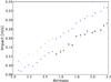 |
Fig. 5 Impact of the atmosphere in the RVs for 18 Sco for different values of airmass. All the spectra were taken during the night of 2012/05/19. The blue dots represent the impact calculated using the default TAPAS spectra, the green crosses (+) in the left part of the plot represent the impact using the TAPAS spectra for the time corresponding to spectra with airmass 1.55, and green + crosses in the right part the impact using the TAPAS spectra for the hour corresponding to spectra with airmass 1.5. The black stars represent the impact using adjusted H2O transmission spectra. |
If one considers the blue dots in Fig. 5, one can see the impact of the atmosphere depends on the airmass. One can easily see that the impact seems to be linearly proportional to the airmass, except for airmasses around 1.5, where one can observe a jump in the impact value. This jump might be because the data used in the TAPAS atmospheric model is obtained only every six hours. Thus, although one of TAPAS input parameters is the exact hour of the observation, the atmospheric output will be based on an approximated hour, and for one full night of observations, one will have at most three different modeled atmospheric spectra.
To test that the jump in the impact around airmass =1.5 was due to a change in the atmospheric data, we repeated our calculation, now using TAPAS spectra with a wrong time of observation: we used the a TAPAS spectra with the time stamp of the stellar spectrum with airmass =1.55 for the correction of the stellar spectra with airmass ≤1.5 (left part of Fig. 5), and TAPAS spectra with the time stamp corresponding to the spectrum with airmass of 1.5 for the correction of the stellar spectra with airmass ≥1.5 (right part of Fig. 5). By doing so we end up with two nearly parallel lines for the impact. Each line corresponds to a correction with a different modeled atmospheric spectrum.
This result corroborates the hypothesis that the original jump in the impact was due to using two different atmospheric data sets. Moreover, we visually checked that the atmospheric lines were being corrected well, and we found that for airmasses greater that 1.5, telluric lines were being over corrected. Thus, for each of these spectra, we adjusted the H2O transmission by using the power law TX(H2O), T being the transmission and X the adjusting factor (Bertaux et al. 2014). To choose the X value that corrected the H2O transmission better, we chose a small part of the spectrum with no stellar lines (λ = 6483.25 − 6490.25Å), and we minimized the standard deviation for this corrected part of the spectrum. The black stars in Fig. 5 show the calculated impact in the RVs, when used for telluric correction the adjusted transmission. We find a difference between the impact calculated with and without adjusted transmission that can go up to 4 cm s-1, which is close to the magnitude of the error of the impact calculation (see Sect. 5).
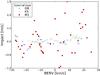 |
Fig. 6 Impact of the atmosphere in the radial velocities for different BERV (barycentric Earth radial velocity) values. A star of spectral type G is represented in small blue dots, a K star in green x crosses, and an M in big red dots. |
Besides studying the effect of the atmosphere on the RV calculation in the night, we also investigated whether the impact of the micro-tellurics would vary along the year for stars of spectral type G8, K5, and M1. For the CCF of the each spectrum, we used the corresponding DRS stellar mask, i.e., for the G8, K5, and M1 stars we used the G2, K5, and M2 masks, respectively. The result is shown in Fig. 6, where one can see the variation in impact of the atmosphere in the RVs calculations with the barycentric Earth radial velocity (BERV) for stars of spectral type G, K, and M. As one has can see in Fig. 3, telluric lines have different impacts depending on the RV of the star. Thus, as the RV of a star changes along the year with respect to the Earth, the impact of the atmosphere also varies as the Earth goes around the Sun, and as the BERV varies. The maximum absolute values of the Impact for these G, K, and M stars is of 31.4, 22.6, and 149.6 cm s-1, respectively. We also calculated the standard deviation (σ) for the relations between the impact and the stellar RV of the G2 synthetic spectra (Fig. 3) and between the impact and the BERV (Fig. 6) for the different spectral types. For the impact G2 star, we present σ for an airmass of 1.0, 1.15, and 2.0. For the stellar spectra obtained with HARPS, we calculated σ considering all the impacts of each star, and also neglecting impacts obtained with airmasses above 1.15 for the G8 and K5 stars and above 2.0 for the M1 star. These values are presented in Table 1. One can see that σ increases since the observations are done with a higher airmass. By considering only observations made with the star at an airmass of less than 1.15, we obtained a difference in σ of 15.1% for the G8 star and of 2.4% for the K5, and neglecting airmasses above 2.0 for the M1 star, we found a difference of 1.6%.
Standard deviation, σ, of the relation between the impact of the atmosphere and the radial velocity of the star, depending on the airmass at the time of the observation.
One should note that the spectra used to calculate the impact for the different spectral types was taken on different nights and at different hours. Therefore, it is difficult to make a direct comparison between the impact of the atmosphere for the different spectral types. Nevertheless, we can envision a periodic variation in the impact with the BERV, which is clearer for the G8 and K5 stars.
5. Discussion and conclusions
With our work we showed that micro-telluric lines should be considered in the calculation of RVs at the level of sub-m s-1. Our test case using synthetic spectra (see Fig. 4) shows a maximum impact of 96.2 cm s-1 for the case in which we have an airmass of 2. This is 46 cm s-1 more than when the star is at its zenith (airmass =1). Thus, even if the 50.1 cm s-1 of impact for the minimum value of the airmass could be explained by systematics, the difference of 46 cm s-1 can only be explained as a consequence of the micro-telluric lines. A 46 cm s-1 impact is whithin the limit of HARPS precision, and is greater than the predicted precision for ESPRESSO. Thus the Earth’s atmospheric absorption should be corrected for when looking for Earth-size exoplanets.
In Sect. 4 we divided HARPS spectra by atmospheric spectra modeled with TAPAS to correct the effect of the micro-telluric lines. When we corrected stellar spectra of one star taken during one night (Fig. 5), we obtained a linear variation of the impact with the airmass, as observed with the synthetic spectra. However, the atmospheric data is only updated every six hours. Therefore the atmospheric spectra used in the correction might not be the spectra corresponding to the exact hour of the stellar observation, and so it may lead to an under-overcorrection of the stellar spectra. This is especially true when there is a change in the weather conditions. This should be the reason for the observed jump of 2.8 cm s-1 in the impact, previously presented in Fig. 5.
The changes in the weather conditions and the airmass variation are not the only factors involved in the micro-telluric effect. As seen in Fig. 6, there is also a variation with BERV, i.e., a periodic variation during the year. This periodic variation is clear, particularly for the G8 and K5 stars. For the M1 star this variation is not so clear. This might be because of the other factors that contribute to the atmospheric impact in the RVs: the spectra were taken during the year, so they were taken on different nights. The ESO atmospheric-conditions archive for La Silla is not always available for the nights of observation, but the most probable scenario is the one in which there are significantly different weather conditions for the several nights. Also, the airmass is not constant, as one can see from Table A.1. Therefore, in addition to the BERV effect, one also have the effect of the other factors that contribute to the impact of the micro-telluric lines on the RV calculation. From Fig. 6 one can also see that the impact of Earth’s atmosphere on RV probably seems more problematic for the M1 star. This can be because of the high airmass values. This star is always near the horizon, so its airmass values are always above 1.7. One way of testing our micro-telluric correction is to calculate the rms for the RV points taken in one night, before and after atmospheric correction. The rms is expected to be smaller after the correction of the atmospheric lines; i.e., the RV points will be less dispersed. Unfortunately, currently available HARPS data do not permit this to be confirmed. We would need asteroseismology time series observation for stars of spectral type K–M, which we expect to suffer a higher contamination from the atmosphere (Fig. 6). But there is no asteroseismology data for stars of these spectral types. We tested then for stars of spectral type G: 18 Sco (G2) and Tau Ceti (G8). Although for some data sets there was, as expected, a decrease in the dispersion, the maximum improvement was marginal: 0.86 cms-1 for 18 Sco and 0.26 cm s-1 for Tau Ceti. With current data we thus cannot completely test the gain when correcting the telluric absorption. The impact of the micro-telluric lines in these G-type stars RV
is in the range 10 − 20 cm s-1, which is lower than the value of HARPS uncertainty along one night (Dumusque et al. 2011). Therefore, it is most probably dominated by instrumentation/calibration noise and not by the atmospheric contamination.
In addition to the factors considered in this work, others should be investigated. Of these we highlight the wind direction and intensity variations, which may induce a shift the atmospheric lines.
We also want to note the lack of error bars in our figures when working with HARPS spectra. Because the impact value is estimated using the same original stellar spectrum with and without atmosphere and the removal of the atmospheric lines is made using an error-free synthetic atmospheric spectrum, the error of the impact will just be the difference between the estimated RV uncertainties for the case with and without atmosphere. To have an idea of these errors, we present the 18 Sco values when the star is at its lowest and its highest airmass. In the first case (airmass =1.070), the error will be of 2.1 cm s-1, and in the second (airmass =2.182) it will be 3.4 cm s-1.
Online material
Appendix A: Star properties
Star properties in our simulations.
Reported in exoplanet.eu in Feb. 25, 2014.
Acknowledgments
We acknowledge support from Fundação para a Ciência e a Tecnologia (FCT, Portugal) through FEDER funds in program COMPETE, as well as through national funds, in the form of grants PTDC/CTE-AST/120251/2010 (COMPETE reference FCOMP-01-0124-FEDER-019884), RECI/FIS-AST/0176/2012 (FCOMP-01-0124-FEDER-027493), and RECI/FIS-AST/0163/2012 (FCOMP-01-0124-FEDER-027492). We also acknowledge support from the European Research Council/European Community under the FP7 through Starting Grant agreement number 239953. N.C.S. and P.F. were supported by FCT through the Investigador FCT contract reference IF/00169/2012 and IF/01037/2013 and POPH/FSE (EC) by FEDER funding through the program “Programa Operacional de Factores de Competitividade – COMPETE.
References
- Anglada-Escudé, G., & Butler, R. P. 2012, ApJS, 200, 15 [NASA ADS] [CrossRef] [Google Scholar]
- Bailey, J., Simpson, A., & Crisp, D. 2007, PASP, 119, 228 [NASA ADS] [CrossRef] [Google Scholar]
- Baranne, A., Queloz, D., Mayor, M., et al. 1996, A&AS, 119, 373 [NASA ADS] [CrossRef] [EDP Sciences] [Google Scholar]
- Bertaux, J. L., Lallement, R., Ferron, S., Boonne, C., & Bodichon, R. 2014, A&A, 564, A46 [NASA ADS] [CrossRef] [EDP Sciences] [Google Scholar]
- Butler, R. P., Marcy, G. W., Williams, E., et al. 1996, PASP, 108, 500 [NASA ADS] [CrossRef] [Google Scholar]
- Clough, S. A., Kneizys, F. X., Rothman, L. S., & Gallery, W. O. 1981, Proc. SPIE, 277, 152 [NASA ADS] [CrossRef] [Google Scholar]
- Clough, S. A., Iacono, M. J., & Moncet, J.-L. 1992, J. Geophys. Res., 97, 15761 [NASA ADS] [CrossRef] [Google Scholar]
- Cotton, D. V., Bailey, J., & Kedziora-Chudczer, L. 2014, MNRAS, 439, 387 [NASA ADS] [CrossRef] [Google Scholar]
- Cunha, D., Figueira, P., Santos, N. C., Lovis, C., & Boué, G. 2013, A&A, 550, A75 [NASA ADS] [CrossRef] [EDP Sciences] [Google Scholar]
- Dumusque, X., Udry, S., Lovis, C., Santos, N. C., & Monteiro, M. J. P. F. G. 2011, A&A, 525, A140 [NASA ADS] [CrossRef] [EDP Sciences] [Google Scholar]
- Dumusque, X., Pepe, F., Lovis, C., et al. 2012, Nature, 491, 207 [NASA ADS] [CrossRef] [PubMed] [Google Scholar]
- Figueira, P., Pepe, F., Lovis, C., & Mayor, M. 2010, A&A, 515, A106 [NASA ADS] [CrossRef] [EDP Sciences] [Google Scholar]
- Figueira, P., Kerber, F., Chacon, A., et al. 2012, MNRAS, 420, 2874 [NASA ADS] [CrossRef] [Google Scholar]
- Kupka, F., Piskunov, N., Ryabchikova, T. A., Stempels, H. C., & Weiss, W. W. 1999, A&AS, 138, 119 [NASA ADS] [CrossRef] [EDP Sciences] [MathSciNet] [PubMed] [Google Scholar]
- Kupka, F. G., Ryabchikova, T. A., Piskunov, N. E., Stempels, H. C., & Weiss, W. W. 2000, Balt. Astron., 9, 590 [NASA ADS] [Google Scholar]
- Marcy, G. W., & Butler, R. P. 1992, PASP, 104, 270 [NASA ADS] [CrossRef] [Google Scholar]
- Mayor, M., & Queloz, D. 1995, Nature, 378, 355 [NASA ADS] [CrossRef] [Google Scholar]
- Mayor, M., Pepe, F., Queloz, D., et al. 2003, The Messenger, 114, 20 [NASA ADS] [Google Scholar]
- Morton, D. C. 1991, ApJS, 77, 119 [NASA ADS] [CrossRef] [Google Scholar]
- Pepe, F., Mayor, M., Galland, F., et al. 2002, A&A, 388, 632 [NASA ADS] [CrossRef] [EDP Sciences] [Google Scholar]
- Pepe, F. A., Cristiani, S., Rebolo Lopez, R., et al. 2010, in Proc. SPIE, 7735, 0F [Google Scholar]
- Piskunov, N. E., Kupka, F., Ryabchikova, T. A., Weiss, W. W., & Jeffery, C. S. 1995, A&AS, 112, 525 [NASA ADS] [Google Scholar]
- Ryabchikova, T. A., Piskunov, N. E., Kupka, F., & Weiss, W. W. 1997, Balt. Astron., 6, 244 [NASA ADS] [Google Scholar]
- Seifahrt, A., Käufl, H. U., Zängl, G., et al. 2010, A&A, 524, A11 [NASA ADS] [CrossRef] [EDP Sciences] [Google Scholar]
- Sneden, C. A. 1973, Ph.D. Thesis, The University of Texas at Austin, USA [Google Scholar]
- Vacca, W. D., Cushing, M. C., & Rayner, J. T. 2003, PASP, 115, 389 [NASA ADS] [CrossRef] [Google Scholar]
All Tables
Standard deviation, σ, of the relation between the impact of the atmosphere and the radial velocity of the star, depending on the airmass at the time of the observation.
All Figures
|
Fig. 1 Normalized synthetic atmospheric spectra obtained with TAPAS (top black line) and LBLRTM (bottom dashed black line). The thick vertical green lines represent the position, for a velocity V = 0, of stellar lines in the G2 stellar mask used by HARPS, and its intensity the weight in the CCF. |
| In the text | |
|
Fig. 2 Normalized spectrum of the spectral type O5 HD 46223 star (blue); normalized spectrum of the spectral type O5 star HD 46223 divided by the atmospheric spectrum obtained with LBLRTM (green); normalized spectrum of the spectral type O5 star HD 46223 divided by the atmospheric spectrum obtained with TAPAS (red). |
| In the text | |
|
Fig. 3 Impact of the atmosphere in the RV calculation for airmass values between 1 and 2. The inner line represents the airmass = 1 and the outer the airmass =2. |
| In the text | |
|
Fig. 4 Maximum impact for the different airmass values. |
| In the text | |
|
Fig. 5 Impact of the atmosphere in the RVs for 18 Sco for different values of airmass. All the spectra were taken during the night of 2012/05/19. The blue dots represent the impact calculated using the default TAPAS spectra, the green crosses (+) in the left part of the plot represent the impact using the TAPAS spectra for the time corresponding to spectra with airmass 1.55, and green + crosses in the right part the impact using the TAPAS spectra for the hour corresponding to spectra with airmass 1.5. The black stars represent the impact using adjusted H2O transmission spectra. |
| In the text | |
|
Fig. 6 Impact of the atmosphere in the radial velocities for different BERV (barycentric Earth radial velocity) values. A star of spectral type G is represented in small blue dots, a K star in green x crosses, and an M in big red dots. |
| In the text | |
Current usage metrics show cumulative count of Article Views (full-text article views including HTML views, PDF and ePub downloads, according to the available data) and Abstracts Views on Vision4Press platform.
Data correspond to usage on the plateform after 2015. The current usage metrics is available 48-96 hours after online publication and is updated daily on week days.
Initial download of the metrics may take a while.