| Issue |
A&A
Volume 568, August 2014
|
|
|---|---|---|
| Article Number | A119 | |
| Number of page(s) | 13 | |
| Section | Stellar atmospheres | |
| DOI | https://doi.org/10.1051/0004-6361/201423703 | |
| Published online | 03 September 2014 | |
Stellar physical parameters from Strömgren photometry
Application to the young stars in the Galactic anticenter survey⋆,⋆⋆
1 Departament d’Astronomia i Meteorologia and IEEC-ICC-UB, Universitat de Barcelona, Martí i Franquès, 1, 08028 Barcelona, Spain
e-mail: This email address is being protected from spambots. You need JavaScript enabled to view it.
2 European Southern Observatory, Karl-Schwarzschild-Str. 2, 85748 Garching, Germany
Received: 24 February 2014
Accepted: 14 June 2014
Abstract
Aims. The aim is to derive accurate stellar distances and extinctions for young stars of our survey in the Galactic anticenter direction using the Strömgren photometric system. This will allow a detailed mapping of the stellar density and absorption toward the Perseus arm.
Methods. We developed a new method for deriving physical parameters from Strömgren photometry and also implemented and tested it. This is a model-based method that uses the most recent available stellar atmospheric models and evolutionary tracks to interpolate in a 3D grid of the unreddened indexes [m1], [c1] and Hβ. Distances derived from both this method and the classical pre-Hipparcos calibrations were tested against Hipparcos parallaxes and found to be accurate.
Results. Systematic trends in stellar photometric distances derived from empirical calibrations were detected and quantified. Furthermore, a shift in the atmospheric grids in the range Teff = [7000,9000] K was detected and a correction is proposed. The two methods were used to compute distances and reddening for ~12 000 OBA-type stars in our Strömgren anticenter survey. Data from the IPHAS and 2MASS catalogs were used to complement the detection of emission line stars and to break the degeneracy between early and late photometric regions. We note that photometric distances can differ by more than 20%, those derived from the empirical calibrations being smaller than those derived with the new method, which agree better with the Hipparcos data.
Key words: methods: observational / techniques: photometric / catalogs / Galaxy: stellar content / Galaxy: structure
Appendices are available in electronic form at http://www.aanda.org
The catalog of the physical parameters is only available in electronic form at the CDS via anonymous ftp to cdsarc.u-strasbg.fr (130.79.128.5) or via http://cdsarc.u-strasbg.fr/viz-bin/qcat?J/A+A/568/A119
© ESO, 2014
1. Introduction
The spiral-arm structure of the Galaxy is an important factor for studying the morphology and dynamics of the Milky Way. We still lack a complete theory to describe its nature, origin and evolution, however. The Perseus spiral arm, the nearest spiral arm outside the solar radius, has been studied through HI neutral gas (Lindblad 1967), large-scale CO surveys (Dame et al. 2001), star-forming complexes (Russeil 2003), or open clusters (Vázquez et al. 2008), among others. These studies traced the arm in the second and third quadrant, but there are very few analysis linking the two quadrants, and pointing toward ℓ ~ 180°. Our project aims to fill this gap, that is, to trace the Perseus arm in the anticenter direction, both in terms of density and kinematics. We examine: 1) the stellar overdensity associated with the spiral arm; 2) the position of the dust layer relative to the arm; and 3) the radial velocity perturbation associated with the arm which will shed light on the mechanisms driving them (e.g., Sellwood 2011; Roca-Fàbrega et al. 2013).
We selected intermediate young stars (B4-A3) for this project. These stars are bright enough to reach large distances in the anticenter direction and old enough to have had time to respond to the spiral-arm perturbation. From stellar evolutionary models (Bertelli et al. 2008) we know that these stars have main-sequence lifetimes in the range 60−700 Myr. Test-particle simulations evolving in a realistic Milky Way spiral-arm potential demonstrated (e.g., Antoja et al. 2011) that a young population – with ages even younger than 400 Myr – have had enough time to develop a clear stellar response to the potential spiral perturbation. This response is observed both in terms of stellar overdensity – redistributing the disk mass and tracing the spiral structure – and in terms of the induced kinematic perturbation, for instance, driving secular changes in the orbits of stars or generating kinematic substructure (such as moving groups). Furthermore, as will be discussed in our next paper (Monguió et al., in prep.), this population is also not old enough to have been significantly affected by disk heating and therefore has a relative low intrinsic velocity dispersion. Because of this lower dispersion, this population will respond more strongly to spiral perturbations which allows detecting weaker spiral amplitudes.
Strömgren photometry is well suited to select these stars and obtain the necessary stellar physical parameters (SPP). For that purpose, we conducted a deep photometric survey in the anticenter direction using the Wide Field Camera at the Isaac Newton Telescope. We obtained full uvbyHβ photometry for 35 974 stars (see Monguió et al. 2013, Paper I hereafter).
In the current paper we focus on deriving the SPP for young stars from Strömgren photometry. Our main goal is deriving accurate distances and reddening for faint stars (up to ). As discussed in Clem et al. (2004), the empirical calibrations available up to now are derived from a small number of stars located in the solar neighborhood (usually clusters), which means that extrapolating these calibrations to large distances is not straightforward. We reviewed the classical methods based on pre-Hipparcos empirical calibrations (EC method hereafter, e.g., Crawford (1978, 1979) or references in Figueras et al. (1991), among others) by comparing photometric distances derived from them with Hipparcos parallaxes. But, we here proceed with a completely different approach. We developed a new model-based (MB) method using theoretical atmospheric grids and stellar evolutionary models. At present, the Strömgren photometric grids available from model atmospheres (Smalley & Kupka 1997; Castelli & Kurucz 2004, 2006) cover a broad range of the stellar parameter space, which makes this approach feasible today.
In Sect. 2, we describe EC and MB methods. In Sect. 3 they are applied to Hipparcos data with the aim of checking and improving the calibrations. Biases and trends are discussed in this section. A rigorous statistical treatment requires estimating individual errors for all the SPP to reach a good and precise error estimate in the photometric distances and reddening. We present a Monte Carlo method that accounts for this. In Sect. 4 the SPP for the OBA-stars in the Galactic anticenter survey are computed, and the results for the two methods are compared. External data provided by 2MASS and IPHAS add information to the survey, which is useful for detecting emission line stars and for defining reliability indexes that list inconsistencies between different sets of data. Finally, we summarize the main conclusions and results in Sect. 5.
2. Methods for computing the SPP
2.1. Classical method: based on empirical calibrations
Several empirical calibration methods are available for computing the SPP from the Strömgren photometric indexes. These procedures follow two steps: 1) the classification of the stars in different photometric regions; and 2) the use of empirical calibrations to obtain the intrinsic indexes and the absolute magnitudes from which interstellar extinction and distances can be computed. From these, Teff and log g have usually been obtained using the atmospheric grids (e.g., Moon & Dworetsky 1985), whereas ages and masses have been obtained from stellar evolutionary models (e.g., Asiain et al. 1997). Here we evaluated these calibrations that provide distances and interstellar extinction, which are necessary parameters for detecting the Perseus spiral arm.
2.1.1. Classification methods
Strömgren (1966) classified the stars in different photometric regions according to their spectral type: the early region (B0-B9), the intermediate region (A0-A3), and the late region, subdivided into three subregions, A3-F0, F0-G2, and later than G2. Later on, Lindroos (1980, LI80) and Figueras et al. (1991, FTJ91) published minor changes with the main differences being in the gap between the early and late regions in the [m1] − [c1] plot1 of reddening-free indexes (Strömgren 1966; Crawford & Mandwewala 1976). Figure 1 shows the [m1] − [c1] plot for the stars in our anticenter survey, which reach magnitudes up to . While these methods provide almost equivalent assignments when the stars in the early and late regions are clearly separated (i.e., for small photometric errors), two important drawbacks have been detected for faint stars with substantial photometric errors (see Figs. 3 and 4 from Paper I). First, LI80 erroneously assigned stars in the gap, i.e., for low [c1] values, to the intermediate region (see Fig. 1 top-right). Second, FTJ91 erroneously classified stars with [m1] > 0.16 and high [c1] values, that clearly belong to the intermediate or late regions, as early-region stars (see Fig. 1 top-left). To remedy that, two additional conditions are included in the classification scheme (indicated in red in Fig. 2). The application of this new classification method (NC) to our anticenter survey is shown in Fig. 1 bottom, where we can observe that the two errors have been corrected.
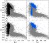 |
Fig. 1 [m1] − [c1] diagram for all the stars in the anticenter survey. The stars are plotted in gray and the overplotted colors show different regions: the early region in black, the intermediate region in blue. The classifications applied are those from FTJ91 (top-left), LI80 (top-right) and NC (bottom). |
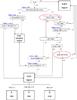 |
Fig. 2 Scheme of the new classification method. Red circles indicate new criteria added to previous classification methods. In blue, reference tables from Strömgren (1966). |
2.1.2. Empirical calibrations
Several calibrations have been published in the past fifty years. An exhaustive pre-Hipparcos compilation was published by Figueras et al. (1991). Later on, some post-Hipparcos calibrations have been established, but all of them concerning F-G late-type stars (e.g., Holmberg et al. 2007; Karataş & Schuster 2010). In the present work, to derive the SPP of stars earlier than A9 we reviewed the following most often used calibrations: Crawford (1978, CR78), Lindroos (1981, LI81) and Balona & Shobbrook (1984, BS84) for the early region; Claria Olmedo (1974, CL74), Grosbøl (1978, GR78), Hilditch et al. (1983, HI83), and Moon & Dworetsky (1985, MO85) for the intermediate region; and Crawford (1979, CR79) for the late region up to A9.
2.2. New strategy: the model-based method
In this section we propose a new method based on the most upgraded theoretical atmospheric grids and evolutionary models. This new approach is, by construction, completely independent of the previously used classical method. As input data, it simultaneously uses the three extinction-free photometric indexes [m1], [c1], and Hβ. First, after an a priori selection of the metallicity of the star, a 3D fit in the theoretical [m1] − [c1] − Hβ plane derived from the atmospheric grid allows us to determine log g and Teff, the intrinsic colors, and the bolometric correction  . The absorption
  is then easily estimated from the observed color index. As a second step, an interpolation in the stellar evolutionary tracks provides the luminosity (L/L⊙), the mass, and the age of the star. For this, we used the interpolation code developed by Asiain et al. (1997). This luminosity is then translated into bolometric magnitude following
  . Finally, the distance is computed using the BC, the AV, and the apparent V magnitude.
The most recent atmospheric grids are those from Castelli & Kurucz (2004, 2006) using ATLAS9 and the mixing length theory2. For each grid point, the authors provide Teff, log g, unreddened indexes ((b − y),m1,c1 and Hβ) and bolometric correction (BC). A different set of grids was previously published by Smalley & Kupka (1997, hereafter SK97), using in this case turbulent convection models for late-type stars from Canuto & Mazzitelli (1991, 1992), which have significant differences from the first one. Unfortunately, SK97 do not provide the Hβ values, therefore a direct comparison of the results has only been possible by combining SK97 data with the Hβ values from Castelli & Kurucz (2006) or from Smalley & Dworetsky (1995), who also used Kurucz (1979) grids and the mixing length theory. When we compared the two sets we found differences of up to 0 025 in (b − y)0 and 006 in c1 for cold stars. Differences for hot stars were always smaller that 002. Differences in m1 are small for low gravities and low Teff, but then they increase up to 003 for log g = 4.5 − 5. The differences between different grids are revisited in Sect.3.2.
Before this method is applied, it is important to analyze what it requires by way of an a priori knowledge of the star’s metallicity. This parameter is needed to select the atmospheric grid and the evolutionary model to be used. We checked that the degeneracy in the [m1] − [c1] − Hβ for several metallicities is too high to derive this parameter simultaneously with the other SPP. Thus, this possible drawback has to be properly analyzed. We identified two options. First, for the stars A3-A9 in the late region it is possible to derive [Fe/H] from the photometric indexes using empirical calibrations (see Schuster & Nissen 1989, and the references therein), which means that in this case one could use its corresponding interpolated grids and evolutionary models. Second, one can consider different a priori values for the metallicity of the star (or the working sample) and quantify whether the changes in SPP values are significant. We considered this second option when applying the MB method to our anticenter survey from Paper I. These stars have distances of about 3−4 kpc toward the Galactic anticenter. Assuming a radial metallicity gradient of about −0.1 dex/kpc – indeed a very uncertain parameter at present – the metallicity of the stars in the sample will mostly be in the range [0, −0.5] dex. SPP data were computed using the Castelli grids available for [Fe/H] = −0.5 and [Fe/H] = 0.0. We checked that for hot stars (Teff> 7000 K), the differences in [m1] and [c1] are smaller than 002 and the differences in Hβ smaller than 001, that is, they are on the same order of the photometric errors. On the other hand, we mention that the EC method is not free from this drawback. Although empirical calibrations for deriving [Fe/H] are available in the literature, the intrinsic indexes and absolute magnitude are usually calibrated from a solar neighborhood sample (see Sect. 2.1), therefore equivalent trends and biases can be expected when this is applied to the most distant stars.
The 3D fitting algorithm we developed (see Appendix A) maximizes the probability for one star to belong to a point of the [m1] , [c1] ,Hβ theoretical grid. It takes into account the distance between them as well as the photometric errors in the three indexes, which are assumed to be Gaussian. We took into account that stars in the gap between the early and late regions can have a two-peak probability distribution, that is, they can belong to either one or the other side of the gap. To keep track of this, both the first (Pmax) and secondary ( ) maximum probabilities are stored together with their corresponding SPP. When
  is close to one, that is, when a star has similar probabilities to belong to the early or late regions, these probabilities allow us to detect the ambiguity and to point out the need for additional information (e.g., 2MASS; see Sect. 4.2) for the final assignment of the SPP.
After Teff, log g, and BC were derived, the stellar evolutionary models of Bertelli et al. (2008, 2009) were used to derive the visual absolute magnitude, and in turn the stellar distance. For a fixed metallicity, Bertelli et al. (2008, 2009) provided 32 evolutionary tracks with masses between 0.6 and 20 M⊙. For more massive stars, that is, for stars earlier than ~O8 (not used in our analysis of the spiral-arm overdensity), the Bressan et al. (1993) evolutionary tracks of the same Padova database were implemented. These tracks cover the 20−120 M⊙ range that is not reached by Bertelli et al. (2008, 2009) grids. We used the interpolation code provided by Asiain et al. (1997).
2.3. Errors
The errors for the obtained SPP were estimated through Monte Carlo simulations. For each star, 100 realizations were performed and the corresponding observed parameters were sampled (V, (b − y), m1, c1, and Hβ) assuming random Gaussian errors. The mean and dispersion for each SPP parameter were obtained from these 100 realizations. This procedure was applied to the EC and MB methods. For the EC method one could also follow the strategy proposed by Reis & Corradi (2008, for B-type and Knude (1978, for A-type stars), which is based on the error propagation in the empirical relations. We note several advantages of the Monte Carlo method proposed here: 1) it provides a better consistency between the errors computed from EC and MB, an important fact when trying to test these two methods against Hipparcos data (Sect. 3); 2) this error computation process applied to the EC method also provides a parameter related to the probability of the star to be assigned to a region different from the one initially assigned (Nreg), 3) equivalent parameters are obtained for the MB method, that is, the 3D fitting algorithm can assign some of the realizations to the other side of the gap. The parameter Nside indicates the number of realizations located at the same side of the gap and provides an additional flag that accounts for a good assignment.
A large portion of the stars in our samples may be binaries, which can include a bias in the distances when we treat them as single stars. The effects of this bias are discussed in Appendix B, where some simulations were made to understand the variation in the photometric indexes caused by a secondary star. The larger biases are for mass ratios close to M2/M1 ~ 1, giving upper limits of 005 for [c1], 002 for [m1], and 004 for Hβ for stars with Teff> 7000 K. In that case, the error in apparent magnitude can reach 075, that is, a 30% error in distance.
3. Testing photometric distances using HIPPARCOS data
Hipparcos data were used here to determine whether the EC and MB methods can derive good stellar distances. Because we are dealing with nearby stars, interstellar extinction plays a secondary role and calibrations used to derive AV cannot be tested. We need to detect, evaluate, and correct for, when possible, the systematic trends observed when comparing trigonometric and photometric distances. Hipparcos OBA-type stars with Strömgren indexes from Hauck & Mermilliod (1998) were taken from the compilation of Torra et al. (2000) – for the OB stars – and Asiain (1998) – for A type stars. The final sample contains 4601 OBA with parallaxes and all photometric indexes (including Hβ): 91 O-stars, 2568 B-stars, 1574 A0-A3 stars, and 368 A4-A9. The spectral type was taken from the Hipparcos Input Catalog (HIC).
To undertake this analysis it is important to work in the space of the observables. To do this, we compared the methods in terms of parallaxes (π), and not in terms of distances (r). As is known, whereas the error in the Hipparcos trigonometric parallax is symmetric, the corresponding error in distance is not (Luri & Arenou 1997). Our strategy was to check the difference between the photometric and the trigonometric parallax (πpho − πhpc) against trigonometric parallaxes (πhpc). We preferred the trigonometric parallax in the abscissa axis because it has a constant absolute error, which is a more clear and understandable behavior. Figure 3 shows the scheme of the considerations that were taken into account in this comparison. First, whereas the absolute error in trigonometric parallax is constant, that is, it does not depend on parallax, photometric parallaxes have, by construction, a constant relative error, in other words, an absolute error that linearly depends on parallax. The propagated error on the difference (πpho − πhpc) is the convolution of both (see black curve in Fig. 3). On the other hand, we know that while about 3% of our sample have negative trigonometric parallaxes (removed from the sample), photometric parallaxes are always, again by construction, defined positive. Although statistically some negative values for small photometric parallaxes (large distances) are expected, we forced all the photometric parallaxes to be positive. This creates a forbidden region below the line of 45° (shown as a dashed line in Fig. 3) because the differences (πpho − πhpc) will be always larger than (−πhpc). The effects caused by this constraint were taken into account by avoiding the smallest parallaxes – the entire analysis was made considering πhpc< 3 mas – and by working with medians instead of means. The first condition allowed us to remove stars with significant interstellar extinction. The analysis was made separately for each of the Strömgren regions (early, intermediate, and late) separately. To have a significant number of stars per bin when computing medians, we constrained the analysis to stars with πhpc< 10 mas for the early region (O-B9), πhpc< 15 mas for the intermediate, and πhpc< 20 mas for the late group (A3-A9). Results are presented in Figs. 4 and 5.
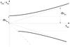 |
Fig. 3 Scheme of the expected distribution of (πpho − πhpc) vs. πhpc. Here we assume a constant absolute astrometric standard error in the trigonometric Hipparcos-based parallax σπhpc. As can be seen in Fig. 17.7 of Hipparcos Catalog this assumption is correct only for bright stars. We checked that the 85% of the stars considered in this analysis, with the requirement to have full Strömgren photometry have , therefore the assumption is acceptable. For photometric parallaxes, a constant relative error is assumed. Again, in this case, as the stars are apparently bright, which means that they are nearby, we assume that reddening effects and a low signal-to-noise ratio do not affect the derived distances. |
3.1. Checking the classical EC method
In Table 1 we detail the median differences between Hipparcos and photometric parallaxes, as well as the trends in Teff, for the different photometric regions. For the early region, CR78 and BS84 give very similar results, with the median close to zero. A clear trend in [c1] – tracing Teff for this region – is present, however, with rhpc<rphot for hotter stars and rhpc>rphot for the colder B-type stars. For the intermediate region, we found very similar results for all the methods, with CL74 and GR78 with a lower error in median, and always obtaining rhpc>rphot. A weak trend in distance is present for all of them, with no clear trend in a = (b − y) + 0.18 ((u − b) − 1.36) – tracing Teff in this region. For the late region up to A9, the CR79 method slightly underestimates the distances with a mild trend in Hβ – the Teff indicator in this region. The calibrations used in the following sections for the EC method give smaller biases, that is, CR78 for the early region, GR78 for the intermediate region, and CR79 for the late region up to A9. The results for these three methods are shown in Fig. 4.
Median differences between Hipparcos and photometric parallaxes in mas.
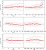 |
Fig. 4 Running median for the difference between EC photometric and Hipparcos parallaxes vs. Hipparcos parallax (left) and vs. Teff photometric index indicator (right). Top: early region using CR78 ([c1] indicating Teff). Middle: intermediate region using GR78 (a indicating Teff). Bottom: late region up to A9 using CR79 (Hβ indicating Teff). The solid line shows the moving median and the dashed line is one standard deviation. Parallaxes are given in mas. |
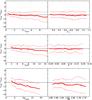 |
Fig. 5 Running median for the difference in parallax vs. Hipparcos parallax (left) and vs. Teff indicator for each region using the MB method (right). Top: early region ([c1] indicating Teff). Center: intermediate region (a indicating Teff). Bottom: late region up to A9 (Hβ indicating Teff). All of them use Castelli grids. The solid line shows the moving median and the dashed line is one standard deviation. Parallaxes are given in mas. |
3.2. Checking the new MB method: Correcting for the atmospheric model
For the MB method we also compared the results for the three photometric regions. For the early region, results give a small bias in parallax of −0.51 mas, but in this case, the trend in effective temperature shown by CR78 is removed (see Fig. 5 top). For the intermediate region, the bias is small (0.03 mas in median), giving better results than the EC method (see Fig. 5 middle). For the late region we found a clear bias between MB and Hipparcos parallaxes with a trend in both parallax and Teff (see Fig. 5 bottom). We have checked that there is also a bias in E(b − y), with clearly negative mean values (−003). The check was repeated using the atmospheric grids by Smalley & Dworetsky (1995) for uvby, with different combinations of the grids by Castelli & Kurucz (2006) and Smalley & Kupka (1997) for the Hβ values, following  (1)These options modify the results for stars with 5500 <Teff< 8500 K in the correct direction. The best results were achieved for the Smalley & Dworetsky (1995) grids for uvby with a combination of the grids of Castelli & Kurucz (2006) and Smalley & Kupka (1997) for the Hβ, with a value of k = 0.2.
From this we suggest that there is a bias in the Castelli grids for late type stars. This problem was solved by creating a new grid as a combination of other available options. The new solution shows no bias, as can be seen in Fig. 6. The new grids were checked only for stars with Teff> 7000 K.
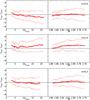 |
Fig. 6 Running median for the difference between MB and Hipparcos parallaxes vs. Hipparcos parallax (left) and vs. Teff indicator for the late region (A3-A9; right). Top: k = 0. Center: k = 1. Bottom: k = 0.2. The solid line shows the moving median and the dashed line is one standard deviation. Parallaxes are given in mas. |
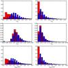 |
Fig. 7 Error distribution for MV, AV and distances obtained with the MB method (red) and EC method (blue). Left: stars with only one measurement. Right: stars with more than one measurement. |
4. SPP for young stars in our anticenter survey
We applied the EC and MB method to the young stars in our Galactic anticenter survey (Paper I). The full catalog contains 35 974 stars with all Strömgren indexes, the extended catalog lists 96980 stars with partial data. The inner 8 and the outer 8 reach ~90% completeness at and
  5, respectively (see Paper I). Photometric internal precisions between 001−002 were obtained for stars brighter than with several measurements, increasing up to 005 for fainter stars with V ~18 (see Fig. 3 in Paper I). During the process of computing the SPP with EC and MB, a discrepancy between the distribution of Hβ values and expected range was detected. This led us to re-check the list of standard stars used3 and the equations for the transformation into the standard system.
In addition, we realized that the equation without (b − y) term (i.e., Eq. (3b) in Paper I) provides more coherent results. Both changes lead to slightly different new values for the Hβ indexes, presented in this new version of the catalog. The current coefficients for the transformation into the standard system are presented in Appendix C.
The EC method was applied to 11854 stars classified as belonging to the early, intermediate, or late regions (<A9) using the NC classification method. This provides intrinsic color, AV, MV, and distances, as well as the corresponding errors. In addition, the catalog provides the photometric region assigned (regNC) and the parameters Nreg and Nregi, which are reliability indicators of this assignment (see Sect. 2.3).
When we applied the MB method to our survey we obtained 13 337 stars with Teff> 7000 K. Distance, intrinsic colors, MV, Teff, log g, age, mass, and BC, together with their corresponding errors, are provided. Additionally, parameters indicating the quality of the 3D fitting (see Sect. 2.3) and the SPP values for the alternative assignment (due to the uncertainty between the early and late regions for faint stars, see Sect. 2.2) are given. The accuracy obtained for MV, AV, and distances are presented in Fig. 7 and are compared with those of the EC method. The errors in distances and MV derived with the EC method are clearly larger than those derived with the MB method. As explained in Paper I, the published error in the observed indexes are the error of the mean for the stars with more than one measurement (32% of the stars), and the standard deviation computed by error propagation when there is only one measurement (68% of the stars). In the first case, the errors in distances are smaller than 20%, while for stars with one measurement, they can reach 40−50% in some cases.
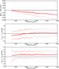 |
Fig. 8 Running median for the differences in distance (top), AV (center) and MV (bottom) obtained from the two methods (EC minus MB) vs. distances from the MB method for the stars in our anticenter survey. The solid line shows the moving median and the dashed line is one standard deviation. |
4.1. Comparison between the MB and EC methods
Figure 8 shows the differences in distance, AV, and MV obtained between the two methods. From this analysis, about 8% of faint stars of the sample were excluded, because they are placed in the gap and the EC and MB methods assign them to different regions. Including them would mask the statistical comparison between the methods. The first important trend observed in these figures is that the EC method gives clearly smaller distances than the MB method. We can state that a systematic difference exists between the two methods, which provides differences in relative distances as large as 20%, that is, differences as large as 300−500 pc can be present near the expected position of the Perseus arm, at about 2−3 kpc. This shift is in the same direction as the clear trend found when comparing EC calibrations and the Hipparcos parallaxes in Table 1 and Fig. 4: the EC provides smaller distances than Hipparcos in most of the cases. This common behavior suggests a possible bias in the EC pre-Hipparcos calibrations published by Crawford in the seventies.
In the MV plots (Fig. 8 bottom) we can quantify this effect in terms of the visual absolute magnitudes. A constant bias in EC, of about 04−05, makes the stars systematically intrinsically faint, that is, more nearby than they really are. The differences observed in AV are smaller (see Fig. 8 middle) with a less significant contribution to the derivation of photometric distances. We observe that, for stars at large distances (>1.5 kpc), the differences in AV between EC and MB are smaller than 0.02 magnitude, that is, they are on the order of the smaller photometric errors. On the other hand, stars at short distances (<1.5 kpc) have differences as large as 005. In Fig. 9 we quantify the differences between the two methods in the intrinsic (b − y)0 color. We separately plot the trends observed inside each photometric region, according to the NC classification. The differences are small, reaching only values up to 0.04 magnitude around A0 and A3 type stars, that is, at the edges between two photometric regions. We consider that this behavior reflects another disadvantage of the empirical calibration methods. By construction, the MB method should not lead to any special jump around A0 and A3, the edges of the Strömgren photometric regions. Thus, the opposite differences observed around these edges in Fig. 9 – with positive or negative differences depending on whether we approach from the left or from the right – will be caused by the EC method. We suggest that calibrations that are valid in the center of the photometric region are erroneously extrapolated to its edges.
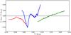 |
Fig. 9 Running median of the differences in (b − y)0 (EC - MB) vs. (b − y)0 for early (red), intermediate (blue), and late-type stars (green). |
4.2. 2MASS data as a reliability test
Almost all the stars in the anticenter survey have 2MASS counterparts (99.3% of the sample). These data were used to detect classification problems in the MB method and to provide a quality flag to the obtained SPP data. The JHK data are less affected by extinction. Using the relations from Rieke & Lebofsky (1985), we computed the expected absorption in the JHK indexes from the AV derived from Strömgren photometry. From this, intrinsic JHK color indexes were computed and compared with the intrinsic Strömgren index (b − y)0 obtained from the MB method. This was made assuming the main-sequence relations (more than 90% of the sample stars have log g> 3) obtained from combining the grids from Bessell et al. (1998) for JHK, and Castelli & Kurucz (2004, 2006) for uvby (see Sect. 2.2). We computed the smallest distance in the (J − K)0 − (b − y)0 and (J − H)0 − (b − y)0 planes (see Fig. 10) between the current location of the star and the expected main sequence, that is, DJK,min and DJH,min. We expect these distances to be small. A very high value for these DJK,min and DJH,min indexes would indicate for most of cases that the Strömgren photometry is not coherent with the 2MASS photometry. These operations were repeated with the  and
and  (i.e., SPP obtained assuming that the star belongs to the other side of the gap), obtaining the values DJK,B,min and DJH,B,min. In principle, the departures from the mean relations should be smaller in the first case, otherwise this would indicate a misclassification problem. These differences FlagJK = DJK,B,min − DJK,min and FlagJH = DJH,B,min − DJH,min were added to the catalog. Seventy-six per cent of the stars have two positive indexes, which indicates that option B results have larger discrepancies, while only around 3% of the stars have FlagJK + FlagJH< − 0.1, which indicates that the first assignment is an incorrect classification; and the SPP computed for the other side of the gap are preferred.
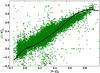 |
Fig. 10 (J − K)0 vs. (b − y)0 plot for the anticenter stars computed following the MB method. The black line shows the expected main sequence obtained by combining grids of the ATLAS9 model atmosphere from Castelli & Kurucz (2004, 2006) and Bessell et al. (1998). |
4.3. Comparison with IPHAS data
Only half of our survey area is covered by the IPHAS initial data release (IDR; González-Solares et al. 2008). Up to 54% of the stars in our survey with full photometry have IPHAS data. The distance for early-A type stars can be estimated from IPHAS data following Sale et al. (2010). The authors suggested to select the early-A stars from a color-color diagram and assumed for them (r − i) = 0.06 and Mr = 1.5. We compared these distances with those derived using MB for the A0-A5 stars in our catalog (see Fig. 11-left). The results give a clear bias of up to 30% with larger IPHAS distances. Taking into account the results from previous sections, we have rEC<rMB<rIPHAS.
IPHAS data also allow us to detect emission line stars by combining our Hβ data and the (r − Hα) index. We consider that a star is an emission line when (r − Hα) > − 0.614 Hβ + 2.164 (see Fig. 11-right). The flag EMLS is included in the catalog. About 5% of the stars with IPHAS data are found to be emission line stars.
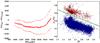 |
Fig. 11 Left: differences between MB and IPHAS distances as a function of the MB distance for early-A type stars (A0-A5). The solid line shows the moving median and the dashed line is one standard deviation. Right: r − Hα vs. Hβ. In red, stars classified as emission line stars. The green line shows the established limit. |
5. Summary and conclusions
We presented a new method for deriving stellar physical parameters from Strömgren photometry. This method uses the three extinction-free photometric indexes ([c1] − [m1] − Hβ) to interpolate in the theoretical atmospheric grids deriving (b − y)0, AV, BC, Teff, and log g. The stellar evolutionary models were then used to obtain MV, distances, ages, and masses. It rigorously takes into account the observational errors in the process, which makes it ideal for deriving physical parameters for stars collected from large and deep photometric surveys. Our study focused on the young and massive stars with Teff> 7000 K (~OBA type stars). Furthermore, 2MASS and IPHAS data were used to complement the results.
We have performed an exhaustive and accurate comparison of this new method with the classical approach, which is based on the use of pre-Hipparcos empirical calibrations, and with distances derived from Hipparcos parallaxes. Substantial differences are present. The most significant trends we found when we compared the empirical calibrations with the Hipparcos parallaxes are 1) a trend in the photometric distance for the early region (O-B9) as a function of [c1] – temperature indicator in this spectral range. For stars with [c1] < 0.2, there is a clear bias in the sense rhpc<rphot, while for stars with [c1] > 0.8 it is the opposite: rhpc>rphot; 2) a bias for the photometric distances for the intermediate and late regions (A0-A9), obtaining always lower values than for Hipparcos distances. During the implementation of the MB method, a significant departure of the new distances from Hipparcos parallaxes was detected in the range of Teff = [9000,7000]. We proposed that this bias is caused by a shift in the theoretical Hβ index of the Castelli & Kurucz (2006) atmospheric grids. Hipparcos distances allowed us to quantify this correction and incorporate it into our code for a proper photometric distance derivation.
The two methods were used to obtain the stellar physical parameters for the OBA-type stars in our Strömgren anticenter survey (Paper I, up to ). The data are published in Appendix D using both methods. Our final catalog contains data for more than twelve thousand OBA-type stars. Substantial differences of about 20% between the two distances are present, with the new method yielding the larger distances (corresponding to 05 in MV). In contrast, the two methods provide almost equal values for the interstellar absorption, with differences always smaller than 002.
In forthcoming papers this information will be used to study the radial stellar distribution with the aim to detect the overdensity due to the Perseus arm. The same data will allow us to create a 3D extinction map in our survey area, and analyze the dust distribution and its relation to the Perseus arm dust layer.
Online material
Appendix A: 3D fitting algorithm
In this section we describe the 3D fitting algorithm developed to maximize the probability for one star to belong to a point of the theoretical grid in the [m1] − [c1] − Hβ space. We took into account the photometric errors in the three indexes that form the so-called ellipsoid of errors, as well as the distance between the star (s) and the point of the grid (g): 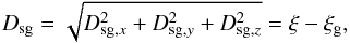 (A.1)with Dsg,x = [c1] s − [c1] g, Dsg,y = [m1] s − [m1] g, and Dsg,z = [Hβ] s − [Hβ] g being the distances in each of the axes, and ξ − ξg being the distance along the axis between the star and the point of the grid.
The propagated photometric error in the direction between the star and the point of the grid (Dse) is computed as the distance between the location of the star and the surface of the ellipsoid of errors in the ξ direction (see Fig. A.1)
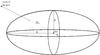 |
Fig. A.1 Schema of the ellipsoid of errors that shows how to compute the σsg between the star and any point of the grid from the individual errors of the three photometric indexes. |
with a = 5σ[c1], b = 5σ[m1], and c = 5σHβ. It is computed from the equation of the ellipsoid and the equation of a line in the ξ direction, that is, 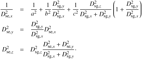 The 5σ photometric error between the star and the ellipsoid in the given direction is
  (A.2)From this, the probability for one star to belong to a point of the grid is computed centered on the star, with the standard deviation being Dse:
 ![Mathematical equation: \appendix \setcounter{section}{1} \begin{eqnarray} P = 1 - \frac{1}{D_{{\rm se}}\sqrt{2\pi}}\left| \int_{-\infty}^{\xi_{\rm g} } \exp \left[\frac{(\xi-\xi_{\rm g} )^2}{2D_{{\rm se}}^2}\right] {\rm d}\xi- \int_{\xi_{\rm g} }^{\infty} \exp \left[\frac{(\xi-\xi_{\rm g} )^2}{2D_{{\rm se}}^2}\right] {\rm d}\xi \right| . \end{eqnarray}](/articles/aa/full_html/2014/08/aa23703-14/aa23703-14-eq138.png) (A.3)For each star, we computed the probability P for all the points of the grid to find the point with higher probability Pmax. In Fig. A.2 we show, for a single star, the probability for all the points of the grid in a [c1]–[m1] and a [c1]–Hβ diagrams.
(A.3)For each star, we computed the probability P for all the points of the grid to find the point with higher probability Pmax. In Fig. A.2 we show, for a single star, the probability for all the points of the grid in a [c1]–[m1] and a [c1]–Hβ diagrams.
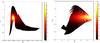 |
Fig. A.2 [c1]–[m1] and a [c1]–Hβ diagram. The color shows the corresponding probability P for a star with ([c1], [m1], Hβ) = (0.96, 0.15, 2.96). |
The original grids are discretized in steps of 0.5 or 0.25 in log g and 250 K, 500 K, or 1000 K in Teff. To develop our 3D fit the grids were interpolated in steps of 10 K in Teff and 0.01 in log g.
Appendix B: Binarity effect
A significant fraction of the young stars in our survey can be binaries, either visual or physical. For physical binaries, some tests were developed to estimate the change in their photometric indexes and in turn the error introduced when ignoring binarity. Their binarity ratio is debated, but according to Arenou (2010) 1) it can reach up to 80% for the more massive stars; and 2) the mass ratio between the stars has a probability peak around M2/M1 = 0.6, with about 10% of cases with a mass ratio higher than M2/M1 = 0.8.
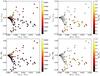 |
Fig. B.1 Differences in [c1] (top) and Hβ (bottom) between the primary and the binary system. Left: the color shows the Teff of the primary. Right: the color shows the mass ratio between the primary and the secondary. |
Simulations were made to estimate the change on the photometric indexes for different mass ratios. Different main-sequence-type stars from B0 to F0 were selected as primaries (checking all the cases, without considering the initial mass function). Then, for each primary, different secondaries were assumed, as well as their physical parameters. We assigned to each star the corresponding photometric indexes ((b − y), m1, c1, Hβ) according to the Castelli & Kurucz (2004) grids, and the assumed Teff and log g = 4.2. Then the fluxes for the primary and the secondary stars were combined. Figure B.1 shows the differences in the photometric indexes between the primary and the combined system for different Teff of the primary and different mass ratios. For primary stars with Teff> 7000 K, the bias reaches values up to 008 in [c1], up to 002 in [m1], and up to 004 in Hβ, which also leads to possible misclassifications. As is known, the effect on absolute magnitude MV is highest when the two stars have equal luminosities, yielding an error of 075 (i.e., 30% error in distance for this extreme case).
Appendix C: New transformation coefficients
The transformation coefficients obtained for the new calibration after modifying the primary standard list are provided in Table C.1. These values have to be compared with those from Tables A.3 and A.4 from Paper I. Equation numbers refer to those from Paper I. The new photometric indexes have also been uploaded to the CDS archive.
Standard transformation coefficients for the new calibration.
continued.
Appendix D: Catalog of young stars
In Table D.1 we describe the columns available for the SPP catalog of our anticenter survey. The complete catalog can be found at the CDS data archive. First an identifier and RA-Dec coordinates for the star are given, as well as the photometric indexes (with the new value of Hβ) and their errors. Then all the SPP from the MB and EC methods are listed, also with the errors and flags. For the MB, the (B) SPP obtained from the second maxim probability at the other side of the gap between early- and late-type regions are also provided. Only the 13687 stars with either Teff> 7000 K from MB or classified as O-A9 by EC methods are included in the catalog. The physical parameters for stars with Teff< 7000 K (either as a secondary (B) SPP or for stars differently classified by the two methods) are only tentative, and they must be used with caution.
Description of the columns available for the SPP catalog.
[m1] = m1 + 0.33 (b − y) and [c1] = c1 − 0.19 (b − y).
An emission line star (S3R1N4), a possible T-Tauri variable star (S4R2N12), stars with an inconsistent Hβ value (S3R2N8 and S3R2N7) and stars with large discrepancies between differences sources of information (S2R2N46, S2R1N25 and S3R1N13) were rejected from the list of standards. ID labels correspond to Marco et al. (2001).
Acknowledgments
This work was supported by the MINECO (Spanish Ministry of Economy) – FEDER through grant AYA2009-14648-C02-01 and CONSOLIDER CSD2007-00050. M.Monguió was supported by a Predoctoral fellowship from the Spanish Ministry (BES-2008-002471 through ESP2006-13855-C02-01 project).
References
- Antoja, T., Figueras, F., Romero-Gómez, M., et al. 2011, MNRAS, 418, 1423 [NASA ADS] [CrossRef] [Google Scholar]
- Arenou, F. 2010, GAIA-C2-SP-OPM-FA-054, http://www.rssd.esa.int/doc_fetch.php?id=2969346 [Google Scholar]
- Asiain, R. 1998, Ph.D. Thesis, Universitat de Barcelona, Spain [Google Scholar]
- Asiain, R., Torra, J., & Figueras, F. 1997, A&A, 322, 147 [NASA ADS] [Google Scholar]
- Balona, L. A., & Shobbrook, R. R. 1984, MNRAS, 211, 375 [NASA ADS] [CrossRef] [Google Scholar]
- Bertelli, G., Girardi, L., Marigo, P., & Nasi, E. 2008, A&A, 484, 815 [NASA ADS] [CrossRef] [EDP Sciences] [Google Scholar]
- Bertelli, G., Nasi, E., Girardi, L., & Marigo, P. 2009, A&A, 508, 355 [NASA ADS] [CrossRef] [EDP Sciences] [Google Scholar]
- Bessell, M. S., Castelli, F., & Plez, B. 1998, A&A, 333, 231 [NASA ADS] [Google Scholar]
- Bressan, A., Fagotto, F., Bertelli, G., & Chiosi, C. 1993, A&AS, 100, 647 [NASA ADS] [Google Scholar]
- Canuto, V. M., & Mazzitelli, I. 1991, ApJ, 370, 295 [NASA ADS] [CrossRef] [Google Scholar]
- Canuto, V. M., & Mazzitelli, I. 1992, ApJ, 389, 724 [NASA ADS] [CrossRef] [Google Scholar]
- Castelli, F., & Kurucz, R. L. 2004, IAU Symp., 210, poster A20 [Google Scholar]
- Castelli, F., & Kurucz, R. L. 2006, A&A, 454, 333 [NASA ADS] [CrossRef] [EDP Sciences] [Google Scholar]
- Claria Olmedo, J. J. 1974, Elementos de Fotometria ESTELAR (Venezuela: Instituto Venezolano de Astronomia) [Google Scholar]
- Clem, J. L., VandenBerg, D. A., Grundahl, F., & Bell, R. A. 2004, AJ, 127, 1227 [NASA ADS] [CrossRef] [Google Scholar]
- Crawford, D. L. 1978, AJ, 83, 48 [NASA ADS] [CrossRef] [Google Scholar]
- Crawford, D. L. 1979, AJ, 84, 1858 [NASA ADS] [CrossRef] [Google Scholar]
- Crawford, D. L., & Mandwewala, N. 1976, PASP, 88, 917 [NASA ADS] [CrossRef] [Google Scholar]
- Dame, T. M., Hartmann, D., & Thaddeus, P. 2001, ApJ, 547, 792 [NASA ADS] [CrossRef] [Google Scholar]
- Figueras, F., Torra, J., & Jordi, C. 1991, A&AS, 87, 319 [NASA ADS] [Google Scholar]
- González-Solares, E. A., Walton, N. A., Greimel, R., et al. 2008, MNRAS, 388, 89 [NASA ADS] [CrossRef] [Google Scholar]
- Grosbøl, P. J. 1978, A&AS, 32, 409 [NASA ADS] [Google Scholar]
- Hauck, B., & Mermilliod, M. 1998, A&AS, 129, 431 [NASA ADS] [CrossRef] [EDP Sciences] [Google Scholar]
- Hilditch, R. W., Hill, G., & Barnes, J. V. 1983, MNRAS, 204, 241 [NASA ADS] [CrossRef] [Google Scholar]
- Holmberg, J., Nordström, B., & Andersen, J. 2007, A&A, 475, 519 [NASA ADS] [CrossRef] [EDP Sciences] [MathSciNet] [Google Scholar]
- Karataş, Y., & Schuster, W. J. 2010, New A, 15, 444 [NASA ADS] [CrossRef] [Google Scholar]
- Knude, J. 1978, A&AS, 33, 347 [NASA ADS] [Google Scholar]
- Kurucz, R. 1979, ApJS, 40, 1 [NASA ADS] [CrossRef] [Google Scholar]
- Lindblad, P. O. 1967, in Radio Astronomy and the Galactic System, ed. H. van Woerden, IAU Symp., 31, 143 [NASA ADS] [Google Scholar]
- Lindroos, K. P. 1980, Stockholms Obs. Rep., 17, 68 [Google Scholar]
- Lindroos, K. P. 1981, Stockholms Obs. Rep., 18, 134 [NASA ADS] [Google Scholar]
- Luri, X., & Arenou, F. 1997, in Hipparcos – Venice ’97, eds. R. M. Bonnet, E. Høg, P. L. Bernacca, et al., ESA SP, 402, 449 [Google Scholar]
- Marco, A., Bernabeu, G., & Negueruela, I. 2001, AJ, 121, 2075 [NASA ADS] [CrossRef] [Google Scholar]
- Monguió, M., Figueras, F., & Grosbøl, P. 2013, A&A, 549, A78 [NASA ADS] [CrossRef] [EDP Sciences] [Google Scholar]
- Moon, T. T., & Dworetsky, M. M. 1985, MNRAS, 217, 305 [NASA ADS] [CrossRef] [Google Scholar]
- Reis, W., & Corradi, W. J. B. 2008, A&A, 486, 471 [NASA ADS] [CrossRef] [EDP Sciences] [Google Scholar]
- Rieke, G. H., & Lebofsky, M. J. 1985, ApJ, 288, 618 [NASA ADS] [CrossRef] [Google Scholar]
- Roca-Fàbrega, S., Valenzuela, O., Figueras, F., et al. 2013, MNRAS, 432, 2878 [NASA ADS] [CrossRef] [Google Scholar]
- Russeil, D. 2003, A&A, 397, 133 [NASA ADS] [CrossRef] [EDP Sciences] [Google Scholar]
- Sale, S. E., Drew, J. E., Knigge, C., et al. 2010, MNRAS, 402, 713 [NASA ADS] [CrossRef] [Google Scholar]
- Schuster, W. J., & Nissen, P. E. 1989, A&A, 221, 65 [NASA ADS] [Google Scholar]
- Sellwood, J. A. 2011, MNRAS, 410, 1637 [NASA ADS] [Google Scholar]
- Smalley, B., & Dworetsky, M. M. 1995, A&A, 293, 446 [NASA ADS] [Google Scholar]
- Smalley, B., & Kupka, F. 1997, A&A, 328, 349 [NASA ADS] [Google Scholar]
- Strömgren, B. 1966, ARA&A, 4, 433 [NASA ADS] [CrossRef] [Google Scholar]
- Torra, J., Fernández, D., & Figueras, F. 2000, A&A, 359, 82 [NASA ADS] [Google Scholar]
- Vázquez, R. A., May, J., Carraro, G., et al. 2008, ApJ, 672, 930 [NASA ADS] [CrossRef] [Google Scholar]
All Tables
All Figures
|
Fig. 1 [m1] − [c1] diagram for all the stars in the anticenter survey. The stars are plotted in gray and the overplotted colors show different regions: the early region in black, the intermediate region in blue. The classifications applied are those from FTJ91 (top-left), LI80 (top-right) and NC (bottom). |
| In the text | |
|
Fig. 2 Scheme of the new classification method. Red circles indicate new criteria added to previous classification methods. In blue, reference tables from Strömgren (1966). |
| In the text | |
|
Fig. 3 Scheme of the expected distribution of (πpho − πhpc) vs. πhpc. Here we assume a constant absolute astrometric standard error in the trigonometric Hipparcos-based parallax σπhpc. As can be seen in Fig. 17.7 of Hipparcos Catalog this assumption is correct only for bright stars. We checked that the 85% of the stars considered in this analysis, with the requirement to have full Strömgren photometry have , therefore the assumption is acceptable. For photometric parallaxes, a constant relative error is assumed. Again, in this case, as the stars are apparently bright, which means that they are nearby, we assume that reddening effects and a low signal-to-noise ratio do not affect the derived distances. |
| In the text | |
|
Fig. 4 Running median for the difference between EC photometric and Hipparcos parallaxes vs. Hipparcos parallax (left) and vs. Teff photometric index indicator (right). Top: early region using CR78 ([c1] indicating Teff). Middle: intermediate region using GR78 (a indicating Teff). Bottom: late region up to A9 using CR79 (Hβ indicating Teff). The solid line shows the moving median and the dashed line is one standard deviation. Parallaxes are given in mas. |
| In the text | |
|
Fig. 5 Running median for the difference in parallax vs. Hipparcos parallax (left) and vs. Teff indicator for each region using the MB method (right). Top: early region ([c1] indicating Teff). Center: intermediate region (a indicating Teff). Bottom: late region up to A9 (Hβ indicating Teff). All of them use Castelli grids. The solid line shows the moving median and the dashed line is one standard deviation. Parallaxes are given in mas. |
| In the text | |
|
Fig. 6 Running median for the difference between MB and Hipparcos parallaxes vs. Hipparcos parallax (left) and vs. Teff indicator for the late region (A3-A9; right). Top: k = 0. Center: k = 1. Bottom: k = 0.2. The solid line shows the moving median and the dashed line is one standard deviation. Parallaxes are given in mas. |
| In the text | |
|
Fig. 7 Error distribution for MV, AV and distances obtained with the MB method (red) and EC method (blue). Left: stars with only one measurement. Right: stars with more than one measurement. |
| In the text | |
|
Fig. 8 Running median for the differences in distance (top), AV (center) and MV (bottom) obtained from the two methods (EC minus MB) vs. distances from the MB method for the stars in our anticenter survey. The solid line shows the moving median and the dashed line is one standard deviation. |
| In the text | |
|
Fig. 9 Running median of the differences in (b − y)0 (EC - MB) vs. (b − y)0 for early (red), intermediate (blue), and late-type stars (green). |
| In the text | |
|
Fig. 10 (J − K)0 vs. (b − y)0 plot for the anticenter stars computed following the MB method. The black line shows the expected main sequence obtained by combining grids of the ATLAS9 model atmosphere from Castelli & Kurucz (2004, 2006) and Bessell et al. (1998). |
| In the text | |
|
Fig. 11 Left: differences between MB and IPHAS distances as a function of the MB distance for early-A type stars (A0-A5). The solid line shows the moving median and the dashed line is one standard deviation. Right: r − Hα vs. Hβ. In red, stars classified as emission line stars. The green line shows the established limit. |
| In the text | |
|
Fig. A.1 Schema of the ellipsoid of errors that shows how to compute the σsg between the star and any point of the grid from the individual errors of the three photometric indexes. |
| In the text | |
|
Fig. A.2 [c1]–[m1] and a [c1]–Hβ diagram. The color shows the corresponding probability P for a star with ([c1], [m1], Hβ) = (0.96, 0.15, 2.96). |
| In the text | |
|
Fig. B.1 Differences in [c1] (top) and Hβ (bottom) between the primary and the binary system. Left: the color shows the Teff of the primary. Right: the color shows the mass ratio between the primary and the secondary. |
| In the text | |
Current usage metrics show cumulative count of Article Views (full-text article views including HTML views, PDF and ePub downloads, according to the available data) and Abstracts Views on Vision4Press platform.
Data correspond to usage on the plateform after 2015. The current usage metrics is available 48-96 hours after online publication and is updated daily on week days.
Initial download of the metrics may take a while.