| Issue |
A&A
Volume 568, August 2014
|
|
|---|---|---|
| Article Number | A23 | |
| Number of page(s) | 6 | |
| Section | Cosmology (including clusters of galaxies) | |
| DOI | https://doi.org/10.1051/0004-6361/201423616 | |
| Published online | 08 August 2014 | |
The insignificant evolution of the richness-mass relation of galaxy clusters
1
INAF – Osservatorio Astronomico di Brera, via Brera 28,
20121
Milano,
Italy
e-mail:
This email address is being protected from spambots. You need JavaScript enabled to view it.
2
Department of Geography, Queen Mary University of
London, Mile End
Road, London
E1 4NS,
UK
Received: 11 February 2014
Accepted: 5 June 2014
Abstract
We analysed the richness-mass scaling of 23 very massive clusters at 0.15 < z < 0.55 with homogenously measured weak-lensing masses and richnesses within a fixed aperture of 0.5 Mpc radius. We found that the richness-mass scaling is very tight (the scatter is <0.09 dex with 90% probability) and independent of cluster evolutionary status and morphology. This implies a close association between infall and evolution of dark matter and galaxies in the central region of clusters. We also found that the evolution of the richness-mass intercept is minor at most, and, given the minor mass evolution across the studied redshift range, the richness evolution of individual massive clusters also turns out to be very small. Finally, it was paramount to account for the cluster mass function and the selection function. Ignoring them would lead to larger biases than the (otherwise quoted) errors. Our study benefits from: a) weak-lensing masses instead of proxy-based masses thereby removing the ambiguity between a real trend and one induced by an accounted evolution of the used mass proxy; b) the use of projected masses that simplify the statistical analysis thereby not requiring consideration of the unknown covariance induced by the cluster orientation/triaxiality; c) the use of aperture masses as they are free of the pseudo-evolution of mass definitions anchored to the evolving density of the Universe; d) a proper accounting of the sample selection function and of the Malmquist-like effect induced by the cluster mass function; e) cosmological simulations for the computation of the cluster mass function, its evolution, and the mass growth of each individual cluster.
Key words: galaxies: clusters: general / galaxies: elliptical and lenticular, cD / galaxies: evolution / methods: statistical
© ESO, 2014
1. Introduction
The evolution of the relation between mass and richness in galaxy clusters is interesting for both cosmological and astrophysical reasons. From an astrophysical perspective, more massive clusters tend to have more of everything, and therefore to factor out this obvious (mass) dependence (for example to stack, combine, or compare clusters of different mass), one needs to measure the scaling of richness with mass at the cluster redshift. Since this is usually not available, one needs knowledge of present-day scaling and of its evolution. The evolution of the richness-mass scaling is also interesting per se, because it gives the evolution of the number of galaxies (per unit cluster mass, alias the halo occupation number, Berlind & Weinberg 2002; Lin et al. 2004). If galaxy mergers or infall are important, then the richness-mass scaling should evolve, except for infalling material that has a number of galaxies per unit mass close to the already infallen material.
From a cosmological perspective, one may infer the mass of a cluster from knowledge of its richness (e.g. Andreon & Hurn 2010; Johnston et al. 2007). However, if the cluster has a redshift fairly different from the clusters used to calibrate the relation, knowledge of the evolution is needed. From the inferred masses, one may eventually learn about the cosmological parameters (e.g. Rozo et al. 2010; Tinker et al. 2012). However, if the richness-mass relation evolves, but is taken to be unevolving, or assumed to evolve in a different way than it does, then a bias in the cosmological parameters would result when cosmological samples are calibrated with samples with an un-matched redshift distribution. Knowledge of the evolution of the richness-mass relation is therefore paramount.
The richness-mass scaling is especially interesting when alternative mass proxies (e.g. the X-ray temperature, or the YX parameter, Kravtsov et al. 2006) are unavailable or their measurement is infeasible. This often occurs for clusters at very high redshift; for example at z > 1.45 only one cluster has a measured X-ray temperature (JKCS 041 at z = 1.803, see Andreon et al. 2009, 2014) and hence a computable YX (YX requires the X-ray temperature), but several clusters are known. Unavailability or infeasibility also occurs at lower redshift (e.g. Faloon et al. 2013; Menanteau et al. 2010), because of the cost of following up large cluster samples in X-ray.
The determinations of the evolution of the richness-mass relation require clusters spread over a sizeable redshift range with known masses derived in a uniform way to avoid introducing systematic biases (see e.g. Applegate et al. 2014). Such samples are rare at best, and therefore most previous studies use mass proxies in place of mass, for example X-ray temperature (e.g. Lin et al. 2006; Capozzi et al. 2012). However, any result found using a mass proxy in place of mass is ambigous: an evolution of the richness-mass proxy (e.g. X-ray temperature) relation may be due to the evolution of richness, or the proxy used to infer the cluster mass. A lack of evolution may instead be due to two evolutions that compensate each other. Furthermore, results are sometimes contradictory (e.g. Lin et al. 2004 vs. Lin et al. 2006). Direct masses are therefore needed to make progress in this field.
Lensing masses are starting to be available for cluster samples spread over a redshift range wide enough to probe evolution (Hoekstra et al. 2012; Applegate et al. 2014) and have the advantage of directly measuring mass and removing the ambiguities of previous attempts which were oblided to use mass proxies because of the absence of directly measured masses.
In this work, we measure the evolution of the mass-richness relation using a sample of clusters with directly measured, weak-lensing masses. We also improve on previous studies by adopting fixed, metric apertures to measure richness and mass and by not de-projecting quantities. The use of a fixed (in Mpc) aperture separates the real (if present) evolution at a fixed radius from the one induced by a conspiracy between a possible non-constant richness-radius relation and the well-known pseudo-evolution of the reference radius (e.g. r500) because of the evolving density of the Universe. This is called pseudo-evolution because the radius and the cluster mass would change even if the cluster mass profile would not.
The use of projected quantities mitigates cluster orientation/triaxiality effects, because they are likely similar for both the matter and the galaxy distribution (Angulo et al. 2012). The advantage mainly consists in a simpler analysis, since de-projected quantities would have correlated errors that have to be accounted for in the analysis. For example, if de-projected quantities were used and error covariance ignored, the intrinsic scatter between richness and mass would be spuriously underestimated.
Although the use of directly measured masses is certainly an improvement upon previous studies, current samples with weak-lensing masses have an unknown selection function, as do previous cluster samples selected in other ways and studied in similar contexts (e.g. Lin et al. 2006; Capozzi et al. 2012). In the case of weak-lensing, the shear effect on background galaxies can only be measured for the most massive clusters, making the accessible mass range very narrow and the mean mass of the sample variable with redshift. The presence of this selection function (Gelman et al. 2004; Heckman 1979) complicates the analysis. It is not, however, a unique feature of cluster samples with weak-lensing masses, since almost every other cluster sample has a limiting, mean, or maximal mass that is redshift-dependent, i.e. it includes clusters of a given mass more frequently at some redshifts than at others.
In this paper we perform a first robust assessment of the evolution of the richness-mass relation of galaxy clusters using a sample of 23 clusters with 0.15 < z < 0.55 with weak-lensing aperture masses. Our sizeable sample with directly measured masses highlights the importance of intrinsic scatter, of addressing selection effects in the cluster sample, and of collinearity1 between richness and redshift, none of which have been considered in any previous studies. Our analysis also emphasises the importance of paying attention to the way clusters are selected and of incorporating the selection function into the estimation. Indeed, performing the astronomical measurements is the simplest part of this work.
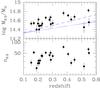 |
Fig. 1 Mass (upper panel) and richness (lower panel) of the studied cluster sample. In the upper panel, the solid/dashed lines indicate the adopted/alternative limiting mass of the selection function. |
Throughout this paper, we assume ΩM = 0.3, ΩΛ = 0.7, and H0 = 70 km s-1 Mpc-1. Magnitudes are in the AB system. We use the 2003 version of Bruzual & Charlot (2003, BC03 hereafter) stellar population synthesis models with solar metallicity and a Salpeter initial mass function (IMF). Results of stochastic computations are given in the form x ± y where x and y are the posterior mean and standard deviation. The latter also corresponds to 68% intervals, because we only summarized posteriors close to Gaussian in that way.
2. Data and sample
2.1. The cluster sample
Our starting point is the Canadian Cluster Comparison Project (CCCP) cluster catalogue (Hoekstra et al. 2012). Fundamentally, the catalogue is a collection of clusters at 0.15 < z < 0.55 with homogeneously derived weak-lensing masses, but without a known selection function. In particular, the catalogue offers the advantageous projected aperture masses within a 0.5 Mpc radius.
We select the subsample observed with the CFHT Megacam camera (Boulade et al. 2003) in two bands bracketing the (rest-frame) 4000 Å break. This gives us a sample of 23 clusters, listed in Table 1, with masses and redshift distributed as in Fig. 1.
In our sample (and in the parent CCCP sample), the mean mass increases with increasing redshift. This is a selection bias, because cluster mass decreases with increasing redshift in individual systems as a result of the continous infall of matter (see Sect. 2.3). The relation is also tight (with a spread of 0.06 dex) because of the combined effect of the steep cluster mass function (at the massive end) and, at the less massive end, the Hoekstra et al. (2012) requirement of dealing with massive clusters only because of the challenging weak-lensing measurements. If the mass redshift trend were scatterless (i.e. these quantities were perfectly collinear), then there would be a strong covariance (degeneracy) between the mass-richness slope and the redshift evolution of the intercept. For example, an unevolving mass-richness scaling would be indistinguishable from a shallower mass-richness scaling joint to an increasing mass with redshift. The degeneracy is broken by the scatter in the M − z relationship, or equivalently M | z, namely mass at a given redshift, i.e. by the vertical width of the mass distribution at a given redshift.
Cluster id, redshift, and projected richness and mass within 0.5 Mpc.
2.2. The data and the derivation of cluster richness
The CFHT Megacam images used in this paper are reduced with MegaPipe (Gwyn 2008). The images are 1 × 1 deg2 wide, have a pixel size of 0.186 arcsec, are taken in sub-arcsec seeing conditions, and are several magnitudes deeper than we need. Specifically, we used g and r photometry for clusters at z < 0.31, r and i for Abell 370 and RXJ1524.6+0957, i and z for Abell 851 and RX J1347.5-1145, and r and z for the remaining clusters.
For each cluster we derived photometry in the two bands using the SExtractor code (Bertin & Arnouts 1996). Total galaxy magnitudes refer to “magauto”, while colours are based on a fixed 3 arcsec aperture.
Basically, we aim to count red members within a specified luminosity range and colour, and within a 0.5 Mpc radius, as already done for other clusters (Andreon 2006, 2008; Andreon et al. 2008; Andreon & Hurn 2010; Andreon & Bergé 2012). We only consider red galaxies because these objects have already exhausted the baryonic reservoir needed to form new stars, and therefore their luminosity evolution is better known. As in Andreon & Hurn (2010), we take a passive evolving limiting magnitude of MV = −20 mag, modelled with a simple stellar population of solar metallicity, Salpeter IMF, from Bruzual & Charlot (2003).
We only count red galaxies, where “red” is defined as in several previous studies (e.g. Andreon et al. 2006; Raichoor & Andreon 2012a,b): redder than an exponential declining τ = 3.7 model, and bluer than 0.1 to 0.2 mag redwards of the colour−magnitude relation. The resulting sample turns out not to depend on the details of the “red” definition because the adopted colour boundaries fall (by design) in regions where no cluster galaxies (in an amount large enough to be detected over the background) are found at the bright magnitude of interest here. Colours are not corrected for the colour−magnitude slope because this is a negligible correction (≲0.1 mag) given the small magnitude range explored and the large color range adopted.
Some of the galaxies counted in the cluster line of sight are actually in the cluster fore/background. The contribution from background galaxies is estimated, as usual, from a reference direction (e.g. Zwicky 1957; Oemler 1974; Andreon et al. 2005). The reference direction is taken outside a radius of 3 Mpc and inside the same Megacam pointing in which the cluster is, hence fully guaranteeing homogeneous data for cluster and control field.
Since weak-lensing masses are computed within a cylinder of 0.5 Mpc radius2, we do the same for richness. The derived (projected) richness values are listed in Table 1 and shown in the bottom panel of Fig. 1. Table 1 shows that richness is quite well measured, since it has on average an error of 17%, very close to mass errors (15% on average). As detailed in the Appendix, richness errors account for Poisson fluctuations in background+cluster counts and the uncertainty on the mean background counts.
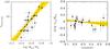 |
Fig. 2 Mass-richness scaling (left-hand panel) and residuals (observed minus expected) as a function of redshift (right-hand panel) accounting for the mass and selection functions. The solid line marks the mean fitted regression line. The shaded region marks the 68% uncertainty (highest posterior density interval) for the regression. In the left panel, measurements are corrected for evolution. |
2.3. Cosmological numerical simulations
The analysis of the real data requires simulated data for computing the mass function (prior), its evolution, and the mass evolution of individual clusters. We use the MultiDark Run 1 dissipationless simulation, described in Prada et al. (2012). This simulation contains about 8.6 billion particles in a volume larger than the Millennium simulation (Springel et al. 2005), and the data are made available in CosmoSim (Riebe et al. 2013). The large volume is useful for giving good statistics for massive clusters like those of interest in this paper. The simulation gives the mass profile of each bound-density-maxima (BDM, Klypin & Holtzman 1997) halo, from which we derived M0.5 accounting for the sligthly different cosmology (WMAP5) adopted in the simulations. After matching each BDM halo with its descendant (via the friend-of-friend halo tree), we derived that log M0.5 increases by ~0.25 dex from z = 0.6 to z = 0. We also derived the mass function (where mass is computed within 0.5 Mpc) to be used as mass prior in our fit. It is very steep at log M0.5/M⊙ ≳ 14.4, i.e. only a tiny range of log M0.5 is accessible, as directly shown by the (real) data in Fig. 1.
3. Results
Following previous works (Lin et al. 2006; Andreon et al. 2008; Capuzzi et al. 2013, etc.) we fit the data with the function: 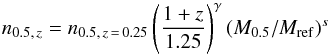 (1)where Mref = 1014.5M⊙. In contrast to these previous studies, we allow a possible log-normal scatter around the mean relation (the scatter is obvious in the Lin et al. 2004 sample), and we prefer to zero-point quantities at z = 0.25 (the median redshift of our sample) instead of at z = 0. We also need to account for the mass function and for the selection function because the Malmquist-Eddington correction (the difference between latent and observed value) depends on the shape of the product of these two functions, see Andreon & Bergé (2012). We therefore take the mass function and its evolution from the Multidark simulation (Sect. 2.3).
As mentioned, the precise expression of cluster selection function is unknown for our cluster sample, mainly because clusters in Hoekstra et al. (2012) have been chosen by the authors amongst a heterogenous and incomplete list of likely massive clusters. We assume that the selection function is sharp (i.e. is a 0/1 function), with a threshold mass, Mthr, linearly increasing with redshift, 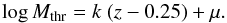 (2)To choose μ and k we note that the lower Mthr is the lower we expect to see data in Fig. 1, (i.e. Mthr cannot be too low), and that Mthr cannot be much higher than the minimal observed mass. We adopted k = 0.5, μ = 14.4 (Fig. 1). A second set of parameters (Fig. 1) are also adopted for assessing sensitivity on this assumption. We quantify the uncertainty induced by the unknown selection function in the Appendix.
The mass-richness-redshift fit results are shown in Fig. 2. We found that richness scales almost linearly with mass (with power s = 1.3 ± 0.3), with negligible intrinsic scatter (log n0.5 | M0.5 < 0.09 dex with 95% probability) and a statistically insignificant evolution (γ = −0.7 ± 0.7). More precisely, 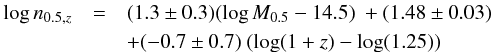 (3)with a strong covariance between s and γ, which inflates the error on γ, meaning that any analysis not accounting for collinearity would derive an overly optimistic γ uncertainty. Instead, the estimated intrinsic scatter is robust against model misfit, because the bulk of the cluster sample has a very narrow distribution in mass (i.e. almost a single value of mass) and a narrow range in redshift, i.e. it does not require any richness-mass-redshift modelling.
The virtual proportionality between richness and mass (slope of their log 1.3 ± 0.3) should not be over-interpreted, as it refers to a very small mass range: 14.4 ≲ log M0.5/M⊙ ≲ 14.8 or 14.6 ≲ log Mvir/M⊙ ≲ 15.5, and we do not know whether the relation continues to be linear or bends at lower masses. Readers having expectations about what the slope of this relation should be, based on relations derived at other radii, should remember that masses at unfixed metric radii, such as M500, are proportional to  with ζ ≠ 1 and that there could be a (perhaps small) radial gradient in N | M.
The γ parameter should not be misunderstood: it measures the evolution of the mass-richness intercept at a given mass. We find a negligible change of −0.09 ± 0.09 dex between z = 0.55 and z = 0.15. It is not a measure of galaxy’s merging rate, but is instead the richness evolution of a fictitious cluster that does not grow in mass. It measures evolution “at a fixed mass”. The evolution of the richness of an individual cluster could be easily derived using Eq. (3) and the mass evolution computed from the MultiDark simulation: 0.11 ± 0.16 dex between z = 0.6 and z = 0. Therefore, in the last 6 Gyr both cluster mass and richness have changed little, if at all. Nevertheless, we emphasise that we would be more sure of our conclusion if we were observing at lower redshift the likely descendants of our clusters at higher redshift, which is surely not the case for current cluster samples, and our sample is no exception.
As mentioned, the selection function is unknown. To assess sensitivity, we adopt an alternative selection function (Fig. 1). We find a relation consistent with Eq. (3). Moreover, the sample selection function is likely to be stochastic: some clusters above the mass threshold are probably missed, and some below the threshold are included (see Andreon & Hurn 2013). To assess the sensitivity of our results to such a possibility, we assumed that the selection function is not a 0 / 1 function, but an error function whose 5 5% probability is represented in Fig. 1 (solid line). We found almost identical parameters, indicating that our results are somewhat robust to uncertainties of the selection function. More tests are given in the Appendix.
4. Discussion and conclusions
We analysed the richness-mass scaling of 23 massive clusters at 0.15 < z < 0.55 with homogeneously derived weak-lensing masses and richnesses within 0.5 Mpc. Our study benefits from: a) weak-lensing masses, preferable to masses derived from a proxy whose evolution is poorly known at best (as, e.g. the X-ray temperature, see Andreon et al. 2011) thereby removing the ambiguity between a real trend and one induced by an accounted evolution of the used mass proxy; b) the use of projected masses that simplify the statistical analysis thereby no longer requiring consideration of the covariance induced by the cluster orientation/triaxiality (not addressed in previous studies); c) a proper accounting of the (Malmquist-like) effect of the cluster mass function and of the selection function, which, if ignored, induce biases comparable or larger than well-measured errors and larger than common-estimated errors (e.g. of those analyses ignoring the collinearity between mass and redshift); d) the use of aperture masses, making clear that the mass change we are talking about is not pseudo-evolution, i.e. a consequence of anchoring the cluster size to the changing density of the Universe, but real evolution resulting from the matter infall; e) the use of MultiDark simulation to quantify the mass growth. Within 0.5 Mpc, it is 0.25 dex between z = 0.6 and z = 0 for very massive clusters. Such a detailed treatment is at best only partially present in studies using popular tools to regress quantities, such as χ2, maximum likelihood, BCES (Akritas & Bershady 1996), FitEXY (Press et al. 1992), or the unpublished Hogg et al. (2010). For example, our mass calibration approach improves upon the Planck Collaboration XX (2014) method, because we account for collinearity and use a directly measured mass instead of a mass proxy. Our approach also improves upon methods used in studies using weak-lensing masses, such as Mahdavi et al. (2013), Israel et al. (2014), von den Linder et al. (2014), Ford et al. (2014), and Sereno et al. (2014), because we model the selection+mass function and account for collinearity. Published works based on calibrations using projected weak-lensing masses are rare at best. Our approach improves upon Hoekstra et al. (2012), because we account for collinearity, Malmquist-bias, and mass+selection functions.
Based on this analysis we find that:
First, there is little, if any, intrinsic scatter between richness and mass (<0.09 dex with 95% probability) when measured in fixed apertures of 0.5 Mpc radius. This implies a tight link between infall/evolution of dark matter and galaxies in the central region of clusters, because a differential infall/evolution of >0.1 dex is detectable (at 95% probability).
We emphasize that the studied clusters have very different morphologies and their evolutionary statuses are different: some of them show a regular morphology and are approximatively spherical, other ones are strongly bimodal (e.g. Abell 223 and Abell 223N or Abell 1758 East and West), very elongated (e.g. Abell 2163), or have complex morphologies. The centre of aperture adopted in Hoekstra et al. (2012), and as a consequence in our work, is put on the obvious cluster centre for regular clusters, but at somewhat different locations for clusters with complex morphologies: at the peak of each sub-cluster in some cases (e.g. Abell 223 and Abell 1758), mid-way between the two peaks in some other cases (e.g. Abell 520), or close to one extreme of the galaxy distribution (e.g. the elongated Abell 2163). The observed small scatter between mass and richness implies that the number of galaxies per unit mass (at the 1.3 power) is independent of morphology and roughly constant almost everywhere in the central region of the cluster, regardless of precisely where this region is taken, and when (i.e. at which evolutionary status) the cluster is observed. Again, this can only occur if the evolution of dark matter and galaxies are closely linked during the cluster merging/accretion, otherwise scatter would be observed.
Second, the evolution of richness at a given mass is −0.15 ± 0.15 dex between z = 0 and z = 0.6. This result is the first robust determination of the evolution of the mass-richness relation. The latter is different from the evolution of the richness of a given cluster because of the evolution of the cluster mass. The change in richness of a given (individual) cluster turns out to be 0.11 ± 0.16 dex in this redshift range. To sum up, there has been little evolution, if any, during the last 6 Gyr, with the caveat that conclusions are derived from a sample whose low redshifts objects are not the descendants of high redshift clusters in the sample, which is potentially risky (Andreon & Ettori 1999).
Third, to provide more precise results, observations of more clusters would be useful, but more clusters with a different, and known, selection function would be better. A wider range of mass is needed to break the collinearity (degeneracy) between mass and redshift (i.e. to decrease the error of evolution of the mass-richness scaling). The fitting model to perform the analysis is, on the other hand, largely set, because we already account for the steep mass function, for the sample selection, for errors on data, for noisiness of mass errors, and for the intrinsic scatter between richness and mass.
Collinearity is the precise term used in statistics to refer to an exact or approximate linear relationship between two explanatory variables, often named “degeneracy” in astronomy. We illustrate the point in the next section.
Sometime referred as “aperture” in Hoekstra et al. (2012).
Acknowledgments
S.A. acknowledge Stephen Gwyn for MegaPipe and for reducing the images of RX J1347, Aniello Grado for his endless efforts in reducing optical images with the purpose of enlarging the cluster sample, Mauro Sereno for highlighting conversations on the subject of this paper, Kristin Riebe for help with dealing with the CosmoSim database, and Alberto Moretti for comments on this paper. We acknowledge CFHT, see full-text acknowledgements at http://www.cfht.hawaii.edu/Science/CFHLS/cfhtlspublitext.html
References
- Akritas, M. G., & Bershady, M. A. 1996, ApJ, 470, 706 [NASA ADS] [CrossRef] [Google Scholar]
- Angulo, R. E., Springel, V., White, S. D. M., et al. 2012, MNRAS, 426, 2046 [CrossRef] [Google Scholar]
- Andreon, S. 2006, MNRAS, 369, 969 [NASA ADS] [CrossRef] [Google Scholar]
- Andreon, S. 2008, MNRAS, 386, 1045 [NASA ADS] [CrossRef] [Google Scholar]
- Andreon, S., & Bergé, J. 2012, A&A, 547, A117 [NASA ADS] [CrossRef] [EDP Sciences] [Google Scholar]
- Andreon, S., & Ettori, S. 1999, ApJ, 516, 647 [NASA ADS] [CrossRef] [Google Scholar]
- Andreon, S., & Hurn, M. A. 2010, MNRAS, 404, 1922 [NASA ADS] [Google Scholar]
- Andreon, S., & Hurn, M. A. 2013, Statistical Analysis and Data Mining, 6, 15 [Google Scholar]
- Andreon, S., Punzi, G., & Grado, A. 2005, MNRAS, 360, 727 [NASA ADS] [CrossRef] [Google Scholar]
- Andreon, S., Quintana, H., Tajer, M., Galaz, G., & Surdej, J. 2006, MNRAS, 365, 915 [NASA ADS] [CrossRef] [Google Scholar]
- Andreon, S., Puddu, E., de Propris, R., & Cuillandre, J.-C. 2008, MNRAS, 385, 979 [NASA ADS] [CrossRef] [Google Scholar]
- Andreon, S., Maughan, B., Trinchieri, G., & Kurk, J. 2009, A&A, 507, 147 [NASA ADS] [CrossRef] [EDP Sciences] [Google Scholar]
- Andreon, S., Trinchieri, G., & Pizzolato, F. 2011, MNRAS, 412, 2391 [NASA ADS] [CrossRef] [Google Scholar]
- Andreon, S., Newman, A. B., Trinchieri, G., et al. 2014, A&A, 565, A120 [NASA ADS] [CrossRef] [EDP Sciences] [Google Scholar]
- Applegate, D. E., von der Linden, A., Kelly, P. L., et al. 2014, MNRAS, 439, 48 [NASA ADS] [CrossRef] [Google Scholar]
- Berlind, A. A., & Weinberg, D. H. 2002, ApJ, 575, 587 [NASA ADS] [CrossRef] [Google Scholar]
- Bertin, E., & Arnouts, S. 1996, A&AS, 117, 39 [NASA ADS] [CrossRef] [EDP Sciences] [Google Scholar]
- Boulade, O., Charlot, X., Abbon, P., et al. 2003, Proc. SPIE, 4841, 72 [NASA ADS] [CrossRef] [Google Scholar]
- Bruzual, G. & Charlot, S. 2003, MNRAS, 344, 1000 [NASA ADS] [CrossRef] [Google Scholar]
- Capozzi, D., Collins, C. A., Stott, J. P., & Hilton, M. 2012, MNRAS, 419, 2821 [NASA ADS] [CrossRef] [Google Scholar]
- Faloon, A. J., Webb, T. M. A., Ellingson, E., et al. 2013, ApJ, 768, 104 [NASA ADS] [CrossRef] [Google Scholar]
- Ford, J., Hildebrandt, H., Van Waerbeke, L., et al. 2014, MNRAS, 439, 3755 [NASA ADS] [CrossRef] [Google Scholar]
- Gelman A., Carlin J., Stern H., & Rubin D. 2004, Bayesian Data Analysis (Chapman & Hall/CRC) [Google Scholar]
- Gwyn, S. D. J. 2008, PASP, 120, 212 [NASA ADS] [CrossRef] [Google Scholar]
- Heckman, J. 1979, Econometrica, 47, 153 [CrossRef] [Google Scholar]
- Hoekstra, H., Mahdavi, A., Babul, A., & Bildfell, C. 2012, MNRAS, 427, 1298 [NASA ADS] [CrossRef] [Google Scholar]
- Hogg, D. W., Bovy, J., & Lang, D. 2010, unpublished [arXiv:1008.4686] [Google Scholar]
- Israel, H., Reiprich, T. H., Erben, T., et al. 2014, A&A, 564, A129 [NASA ADS] [CrossRef] [EDP Sciences] [Google Scholar]
- Johnston, D. E., Sheldon, E. S., Wechsler, R. H., et al. 2007, unpublished [arXiv:0709.1159] [Google Scholar]
- Klypin, A., & Holtzman, J. 1997, unpublished [arXiv:astro-ph/9712217] [Google Scholar]
- Kravtsov, A. V., Vikhlinin, A., & Nagai, D. 2006, ApJ, 650, 128 [NASA ADS] [CrossRef] [Google Scholar]
- Lin, Y.-T., Mohr, J. J., & Stanford, S. A. 2004, ApJ, 610, 745 [NASA ADS] [CrossRef] [Google Scholar]
- Lin, Y.-T., Mohr, J. J., Gonzalez, A. H., & Stanford, S. A. 2006, ApJ, 650, L99 [NASA ADS] [CrossRef] [Google Scholar]
- Mahdavi, A., Hoekstra, H., Babul, A., et al. 2013, ApJ, 767, 116 [NASA ADS] [CrossRef] [Google Scholar]
- Menanteau, F., Hughes, J. P., Barrientos, L. F., et al. 2010, ApJS, 191, 340 [NASA ADS] [CrossRef] [Google Scholar]
- Oemler, A. J. 1974, ApJ, 194, 1 [NASA ADS] [CrossRef] [Google Scholar]
- Planck Collaboration XX 2014, A&A, in press DOI 10.1051/0004-6361/201321521 [Google Scholar]
- Prada, F., Klypin, A. A., Cuesta, A. J., Betancort-Rijo, J. E., & Primack, J. 2012, MNRAS, 423, 3018 [NASA ADS] [CrossRef] [Google Scholar]
- Press, W. H., Teukolsky, S. A., Vetterling, W. T., & Flannery, B. P. 1992, Numerical Recipes (Cambridge: University Press) [Google Scholar]
- Raichoor, A., & Andreon, S. 2012a, A&A, 543, A19 [NASA ADS] [CrossRef] [EDP Sciences] [Google Scholar]
- Raichoor, A., & Andreon, S. 2012b, A&A, 537, A88 [NASA ADS] [CrossRef] [EDP Sciences] [Google Scholar]
- Riebe, K., Partl, A. M., Enke, H., et al. 2013, Astron. Nachr., 334, 691 [NASA ADS] [CrossRef] [EDP Sciences] [Google Scholar]
- Rozo, E., Wechsler, R. H., Rykoff, E. S., et al. 2010, ApJ, 708, 645 [NASA ADS] [CrossRef] [Google Scholar]
- Sereno, M., Ettori, S., & Moscardini, L. 2014, MNRAS, submitted [Google Scholar]
- Springel, V., White, S. D. M., Jenkins, A., et al. 2005, Nature, 435, 629 [NASA ADS] [CrossRef] [PubMed] [Google Scholar]
- Tinker, J. L., Sheldon, E. S., Wechsler, R. H., et al. 2012, ApJ, 745, 16 [NASA ADS] [CrossRef] [Google Scholar]
- von der Linden A., Mantz, A., Allen, S. W., et al. 2014, MNRAS, submitted [arXiv:1402.2670] [Google Scholar]
- Zwicky, F. 1957, Morphological astronomy (Berlin: Springer) [Google Scholar]
Appendix A: Fitting details and systematics
To fit the data, we used an updated version of the Bayesian estimation model in Andreon & Bergé (2012), which already accounts for the presence of a redshift term γ (Eq. (1)), for the cluster mass and selection function, and for the possible presence of an intrinsic scatter. The Andreon & Bergé (2012) model adopts a Gaussian likelihood for richnesses and perfectly measured errors for masses. We therefore replace that part of the model by a more appropriate model, introduced in Andreon & Hurn (2010), which accounts for the non-Gaussian (Poisson) nature of galaxy counts, for the background, and also for the noisiness of the mass errors. We assume a 10% uncertainty on the mass error, see Andreon & Hurn (2010) for details.
To check the fitting model, we generate simulated data for 300 clusters with masses taken from the Multidark simulation and all the remaining quantities (mass errors, relation between richness and mass, richness and mass errors, etc.) from the data. We use a sample which is 15 times larger than the real one to highlight small biases. Using our fitting model, all input parameters are recovered at better than 1σ, i.e. no bias is appreciable for a sample over 15 times larger than the one we are interested in.
If instead the slope were kept fixed during the fitting, as per analyses which have been published so far, we found that the derived γ is biased (as long as the the slope is fixed to a value different from the true slope, of course) and always with an overly optimistic error.
If incorrect mass function and evolution were assumed instead (for example we adopted a fitted mass function one dex off, and evolving five times more slowly than the one used to simulate the data), then the γ term would not be biased by an appreciable amount (by 0.1 to be compared to the 0.7 error of the true cluster sample). This occurs because the Malmquist-Eddington correction depends on the slope of the mass prior (function), not on the absolute value of the mass function (prior), and at these masses the mass function is near to a power law (i.e. a fixed slope function), with a slope nearly independent of redshift. Readers interested in a more details may consult Andreon & Bergé (2012).
With regard to the modelling of the selection function, by adopting μ = 0.7 and k = 14.3, a 0.4 bias in γ is introduced. The latter value is sub-dominant compared to the error on γ of the true sample (0.7). This is, likely, an extreme case because the adopted limiting mass is manifestly too optimistic for the simulated data. Therefore, our results are robust against uncertainties of the selection function. Nevertheless, we emphasize that giving our lack of knowledge concerning the selection function of the real sample, we cannot state this for sure.
Finally, if selection and mass functions are not incorporated anywhere in the analysis, we find a bias (difference between input and fit results) of 0.6 in s and γ. These are, respectively, twice and once the correctly estimated error for the real sample, and between two and six times larger than uncertainties quoted in the analyses neglecting intrinsic scatter and redshift-mass collinearity.
To summarize: firstly, our results are robust to uncertainties of the fitting modelling, including the selection function. Secondly, not addressing the well-known astronomical features (the mass function and the selection function) introduces larger biases than the non-systematic uncertainties for samples as small as ours (23 clusters).
All Tables
All Figures
|
Fig. 1 Mass (upper panel) and richness (lower panel) of the studied cluster sample. In the upper panel, the solid/dashed lines indicate the adopted/alternative limiting mass of the selection function. |
| In the text | |
|
Fig. 2 Mass-richness scaling (left-hand panel) and residuals (observed minus expected) as a function of redshift (right-hand panel) accounting for the mass and selection functions. The solid line marks the mean fitted regression line. The shaded region marks the 68% uncertainty (highest posterior density interval) for the regression. In the left panel, measurements are corrected for evolution. |
| In the text | |
Current usage metrics show cumulative count of Article Views (full-text article views including HTML views, PDF and ePub downloads, according to the available data) and Abstracts Views on Vision4Press platform.
Data correspond to usage on the plateform after 2015. The current usage metrics is available 48-96 hours after online publication and is updated daily on week days.
Initial download of the metrics may take a while.