| Issue |
A&A
Volume 568, August 2014
|
|
|---|---|---|
| Article Number | A124 | |
| Number of page(s) | 11 | |
| Section | Extragalactic astronomy | |
| DOI | https://doi.org/10.1051/0004-6361/201423514 | |
| Published online | 05 September 2014 | |
Detection of galaxies with Gaia
1 Dept. Astronomia, IAG/USP, University of São Paulo, Rua do Matão 1226, 05508-900 São Paulo, SP, Brazil
e-mail: This email address is being protected from spambots. You need JavaScript enabled to view it.
2 Observatoire Aquitain des Sciences de l’Univers, Laboratoire d’Astrophysique de Bordeaux, CNRS-UMR 5804, BP 89, 33271 Floirac Cedex, France
3 SIM – Faculdade de Ciencias da Universidade de Lisboa, Ed. C8, Campo Grande, 1749-016 Lisboa, Portugal
Received: 27 January 2014
Accepted: 16 April 2014
Abstract
Aims. Besides its major objective tuned to detecting the stellar galactic population, the Gaia mission experiment will also observe a large number of galaxies. In this work we intend to evaluate the number and the characteristics of the galaxies that will effectively pass the on-board selection algorithm of Gaia.
Methods. The detection of objects in Gaia will be performed in a section of the focal plane known as the Sky Mapper. Considering the Video Processing Algorithm criterion of detection and the known light profiles of disc and bulges galaxies, we assess the number and the type of extra-galactic objects that will be observed by Gaia.
Results. We show that the stellar disc population of galaxies will be very difficult to observe. In contrast, the spheroidal component of elliptical galaxies and bulges having higher central surface brightness and steeper brightness profile will be easier to detect. We estimate that most of the 20 000 elliptical population of nearby galaxies inside the local region up to 170 Mpc are in a state to be observed by Gaia. A similar number of bulges could also be observed, although the low luminosity bulges should escape detection. About two thirds of the more distant objects up to 600 Mpc could also be detected, increasing the total sample to half a million objects including ellipticals and bulges. The angular size of the detected objects will never exceed 4.72 arcsec, which is the size of the largest transmitted windows.
Conclusions. A heterogeneous population of elliptical galaxies and bulges will be observable by Gaia. This nearby Universe sample of galaxies should constitute a very rich and interesting sample for studying their structural properties and their distribution.
Key words: space vehicles: instruments / techniques: photometric / galaxies: spiral / galaxies: elliptical and lenticular, cD
© ESO, 2014
1. Introduction
The Gaia satellite experiment was launched in December 2013 as part of a mission to produce an all-sky survey with unprecedented angular resolution in the spectral range 330−1000 nm. The selected objects will first pass through the Sky Mapper (SM) section of the focal plane responsible for filtering those objects that in the sequence should be observed in the astrometric field (AF). The expected software-defined magnitude limit of the observable targets in the Gaia photometric system is estimated to be G = 20 mag for point source objects. The satellite is also equipped with two low resolution spectro-photometers operating in the blue spectral region 330−680 nm (BP) and in the red 640−1000 nm (RP) with a typical resolution of 3−27 nm per pixel for the BP photometer and 7−15 nm per pixel for RP.
All the observed objects will have their spectral energy distribution evaluated by these instruments. Moreover, an additional radial velocity spectrograph (RVS) instrument will measure the radial velocity in the calcium triplet region (847−874 nm) for a fraction of the brightest objects with a resolution R = 11 500. The evaluation of the accurate position, distance, and radial velocity for an enormous number of stellar objects will provide extremely useful material to improve our understanding of our Galaxy (Perryman 2001).
Although the mission is focussed on detecting galactic stellar objects, Gaia will also deliver a huge number of detections of non-stellar objects, such as quasars and a particularly interesting data set of galaxies. In the case of nearby galaxies in the local group, it is expected that their brightest stars will also be resolved, providing invaluable information for studying their stellar population and their dynamics. The more distant galaxies will be detected through their diffuse brightest regions, which are mostly concentrated in their central regions. A natural question to ask in this scenario is related to the potential impact of the sample of detected non-resolved galaxies on our comprehension of this subject.
It is clear that the sample of these non-resolved galaxy observations by Gaia will be limited to their very central and bright regions for nearby objects. In each passage of the telescope through these galaxies, the on-board satellite software will sample a small strip of pixels covering the information gathered from a region of 0.59 × 1.77 arcsec (along scan vs. across scan) in the SM section. This region is used to estimate the magnitude of the object and to analyse whether the object should be transferred to the Earth. An important point, however, is that the SM window sent to Earth is larger and will cover a sky size of 4.72 × 2.12 arcsec. Since nowadays most of the morphological information occurring in the disks and bulges of nearby galaxies mainly comes from the observation of regions on much larger angular scales, it is clear that the observed light distribution will be invaluable for morphological studies of the central region of galaxies. This sample will be a complementary set of observations to those that can be obtained from lower resolution Earth-based facilities. However, it is important to mention that these data have reduced spatial resolution, reduced depth, and increased noise since the integration time is 2.9 s, instead of the usual 4.4 s adopted for the AF field. Moreover, the SM window that reaches ground is composed of samples of 2 × 2 binned pixels for G< 16 mag. For G> 16 mag an on-board binning of four regions of 2 × 2 pixels will be applied, resulting in an increase in the total noise. As we show in the next sections, most of the non-resolved galaxies should have G> 16 mag, and therefore the SM Gaia observation of these objects will suffer from these limitations.
Owing to its orbital characteristics, the satellite will regularly observe the same region of the sky each time at different scanning directions. Therefore, it is possible to apply some numerical reconstruction method to obtain estimated two-dimensional images for the observed objects, even though such approaches usually show severe reconstruction artefacts (see Dollet et al. 2005; Harrison 2011, and references therein). Nevertheless, the best angular resolution of Gaia’s AF is 59 mas in the scanning direction, so we should expect that the measurements of the central region of nearby galaxies will be available with very good resolution, quite probably comparable to those available from the HST data and resulting in a larger dataset.
One possible way to evaluate the impact of Gaia observations is through simulating a complete distribution of objects in the Universe including solar system objects, galactic stellar sources and extragalactic sources like galaxies, QSOs and supernovae (Robin et al. 2011). This could be a valuable approach for point-like objects, because the detection of such objects by the Gaia on-board software will be unbiased. Nonetheless, for extended sources, such as other galaxies, this large scale approach is infeasible because it would require that images of all targets be simulated and afterwards passed through the video processing algorithms. In the Robin et al. (2011) simulation, a total of 38 million extragalactic objects were generated with integrated magnitudes G ≤ 20 mag, obeying the observed luminosity functions. This figure could be considered as an upper limit of the possible number of detections by Gaia.
In the present work we explore a complementary view of the extra-galactic science that Gaia may produce and focusing on analysing the possible structural components of galaxies that might be observed by Gaia. The two major components that we study are the disk and the bulge’s spheroidal components. Each of these two basic blocks have been extensively studied in the past decades so their own structural photometric properties is well understood. Given the results discussed in the literature, we then ask the question of what characteristic properties of these two components might be more suited to being detected and selected for transmission to the ground by the satellite.
In Sect. 2 we present some general characteristics of the detection parameters adopted by Gaia that will be more relevant for observing of galaxies. Section 3 discusses the implications for the detection of galaxies constituted by pure stellar disks assuming that those objects are dominated by an exponential surface brightness. Most of the stellar discs have a relatively low surface brightness distribution that will be hard to detect by Gaia. In Sect. 4 we analyse the detections of the spheroidal population located in ellipticals and bulges of spiral galaxies. This component is known to have a much higher central surface brightness and will probably be the major component detected by Gaia. In Sect. 5 we describe the results of a numerical simulation of galaxies obeying the nearby observed brightness profiles. A population of these objects were distributed in a uniform space distribution, and their simulated images pass through a software emulating the same detection procedure as adopted by Gaia. In Sect. 6 we evaluate the effect of increasing the distance in the detection of more distant objects that should be affected by the fixed pixel aperture sampling and cosmological dimming. In Sect. 7 we present our major conclusions.
2. The detection of objects with Gaia
The focal plane of Gaia used for astronomical observations is covered with 106 CCDs having 4500 × 1966 pixels of 10 × 30μm, and the sky will be continuously monitored by the detectors. During its operation the reading of the CCD charges will be synchronized with the speed of the stars crossing the focal plane in a process known as time delay integration (TDI) with a TDI period of 982.8 μs. The resulting angular resolution will be 59 mas, along the scanning direction (AL), and 177 mas in the across scanning direction (AC). The observations of objects is planned in a two-step process. The first pass will be conducted in the section called Sky Mapper (SM) with 14 CCDs where objects will first be detected and then selected for the higher resolution observations in the astrometric field AF section and also in the blue and red photometer sections (BP, RP). Depending on their detected magnitude in the SM section the selected objects with G< 17 mag will also be observed in the radial velocity spectrograph (RVS) responsible for the radial velocity determination.
The functioning of the SM section optimization procedure adopted in the Gaia mission is discussed by Provost et al. (2007) and de Bruijne et al. (2014). Here we only give a very brief resume of this process with emphasis on our present subject of analysis. The first step in a detection will be applied by an algorithm running in the SM section where the video processing unit (VPU) builds a synthetic pixel structure called the SM sample, electronically binning 2 × 2 of the physical Gaia pixels to provide a first lower resolution observation of each potential target in the sky. Each sample of the SM section will be continuously monitored by the video processing algorithm or VPA. Around each sample, the VPA will define two concentric working windows with 3 × 3 and 5 × 5 samples. The detection algorithm will search the inner 3 × 3 windows looking for objects, while the external region of the 5 × 5 windows will be used to determine the sky background. The signal of the external 16 samples of the 5 × 5 working window will be ranked, and the fifth sample with the lowest signal is adopted as the estimated background value. The total flux, F, is defined as the sum of the 3 × 3 working window corrected for the background value and applying a further correction to compensate for the predicted PSF losses of a point source object in the sampled window.
The project evaluation is that on average we should expect that a fraction of 80% of the total stellar flux will be typically detected in the 3 × 3 sample working window, and this figure is used to compensate for the PSF losses. The signal content of each sample (Sij) will be added in the horizontal direction to build three vectors H0, H1, and H2, where Hi = ∑ Sij, as well as along the vertical direction V0, V1 and V2. If H0 ≤ H1>H2 and V0 ≤ V1>V2, then there is a possible condition for an object to be detected in the central sample of this window. Then the two extreme horizontal and vertical vectors will be compared with the total flux to build the quantities H0/F, H2/F, V0/F, and V2/F used as indicators of the PSF shape of each object. Based on the location of each detection in the planes H0/F × H2/F and V0/F × V2/F, the VPA will classify the event either as a (1) particle prompt event (PPE) mostly due to solar protons and galactic cosmic rays; as a (2) ripple region artificially created by the proximity of bright objects; or as a (3) true celestial source generically called a Star. By comparing a large body of simulations (de Bruijne et al. 2014), the Gaia control mission developed a set of numerical relations defining exclusion regions to optimize the Gaia detection of stars. a When there is a positive detection, a small region of the focal plane AF around the object will be delivered to Earth receptors, together with the SM detection region, and will be available for further processing. This limitation in the size of the image sent to Earth is necessary since the transmission of the whole mosaic of CCD frames is not feasible owing to to bandwidth communication restrictions of the satellite operation. The pieces of images of each detection of the same object observed in the AF section will be constituted by a set of binned windows of the standard rectangular Gaia pixels measuring 177 mas across the scanning direction (AC) by 59 mas along the direction of the satellite motion (AL). An important problem from to the previously explained background determination procedure is that the decision of the on-board system to send each section of the image depends not only on their raw magnitude but also on the light gradient due to the illumination on nearby pixels. The expectation is that the adopted VPA detection algorithm will deliver all the stellar objects above the stipulated detection limit assuming a Gaussian PSF having σ = (0.8 − 1.1) × 59 mas with a slight dependence on the stellar colour. For non-stellar images there will obviously be an additional bias against the detection of objects due to the SM adopted background correction (Krone-Martins et al. 2013).
More distant galaxies will be detected by their brightest spots, in most cases restricted to their central regions. The exact properties of the final catalogue of detected objects will clearly depend on additional operational details of the satellite, some of them still under discussion. One interesting task is to estimate which objects of the known nearby galactic population will have more chances of being detected by Gaia. This information is particularly useful for evaluating the probable scientific impact of the Gaia mission on our current understanding of galaxies. Two factors playing a major role in this context are the photometric system and the delivered satellite image resolution. The exact dimensions of the AF section to be sent to earth will depend on the detected flux in the SM section, and for some objects, the AF data it will be binned by the on-board video processing unit (VPU). Basically for brighter objects (G< 13) the full pixel resolution will be preserved in the AF-selected window.
For fainter objects, which is the case for most galactic nuclei, a binning procedure will be adopted in the AC direction keeping the full resolution in the AL direction in order to preserve the final astrometric accuracy of the delivered images. In the AC direction, the process of binning is designed to reduce the read-out noise by directly reading a large block of pixels. The final angular dimension of the transmitted window depends on the estimated object flux in the SM section, as well as in the AF CCD sector column where the high resolution image of the object will be observed. For objects observed in the first AF CCD column (AF1), typical dimensions of the transmitted windows are 1.06 × 2.12 arcsec for objects with G< 13, 0.71 × 2.12 arcsec for 13 <G< 16 and 0.35 × 2.12 arcsec for G> 16. Therefore, since most galactic nuclei regions should have G> 16 mag, the expectation is that only the very central region of nearby galaxies will be available for ground processing of the AF observations. However, as pointed out previously, for each object we will also have the SM sample region covering a size of 4.72 × 2.12 arcsec, therefore providing very useful material for ground processing of the detected images, even if these observations will suffer from an increase in the noise level, as mentioned before.
The photometric system adopted by Gaia is fully discussed in Jordi et al. (2010). The main photometric information is obtained by the unfiltered light from 350 to 1000 nm defining the G magnitude system. Two additional passbands will also be monitored by the blue (BP) and red photometers (RP) measuring the spectral energy distribution for each object through low dispersion optics. The spectral resolution depends on the wavelength. The BP photometer covers the spectral region 330−680 nm with a resolution 3−27 nm/pixel, while the RP photometer will observe in the window 640−1000 nm with a resolution 3−27 nm/pixel. The third instrument will be used for stellar radial velocity determinations in the range 847−874 nm in the region of the Calcium II triplet. Only a fraction of the detected objects will be observed by this instrument. Using the RP data the VPU will estimate the magnitude, GRVS, corresponding to the flux available in the RVS passband. Those objects with GRVS brighter than 17 mag will be observed and the expectation according to Katz et al. (2010) is that objects close to the limiting magnitude should present S/N ≃ 1 in a single transit. However, it is worth mentioning that at the end-of-mission S/N integrated from all the transits will be higher than that, as each object is observed 40 times in average.
The G photometric system is centred at λ0 = 6730 Å with a passband approximately equal to Δλ = 4400 Å. The two closest filters of the Johnson-Cousins system are V (λ0,Δλ = 5510,850 Å) and RC (λ0,Δλ = 6470,1570 Å). Several transformation equations are discussed by Jordi et al. (2010), and their accuracy depends on the colour of the observed stars. For normal galaxies the average colour index of spirals and ellipticals are B − V ≃ 0.4 − 1.0 (Robertson & Haynes 1994). The external region of spiral galaxies is dominated by an stellar disk with a mean colour index B − V = 0.5 ± 0.1 affected by relatively recent episodes of star formation. In the case of S0 and ellipticals, as well as in the classical bulges, the mean colour is B − V = 0.8 ± 0.1, owing to an older stellar population with a mixture of objects having different ages and chemical compositions. Judging from these arguments, the more adequate colour transformation for applying to galaxies are those developed for stars with Te> 4500 K by Jordi et al. (2010):  (1)where the bands BT(λ0,Δλ = 4200, 710) Å and VT(λ0,Δλ = 5320, 980) Å were defined from observations of stars in the Hipparcos catalogue. This system is close to the one of Johnson-Cousins B(λ0,Δλ = 4410,950) Å, V(λ0,Δλ = 5510,1570) Å. According to Jordi et al. (2010), the mean expected residual by adopting this transformation is of the order of 0.03 mag. The photometric transformation adopted in the Tycho catalogue, which is valid in the interval −0.2 < (B − V)T< 1.8, is B − V = 0.850(B − V)T, with an error of 0.05 mag, and V = VT − 0.090(B − V)T, with an error of 0.015 mag. Therefore a stellar object with a colour equivalent to a typical spiral galaxy, B − V = 0.5, should present a magnitude G = V − 0.15 in the Gaia photometric system. For a typical elliptical galaxy with a mean colour index, B − V = 0.8, the corresponding Gaia magnitude should be G = V − 0.26.
As a crude first-order estimation, the adopted criteria for detection implies that the satellite should send objects to Earth with a limiting background-corrected magnitude Glim = 20 mag inside the 3 × 3 sample working window of the Sky Mapper Field (SM) section. We conclude that for close nearby objects the equivalent surface brightness detected by Gaia in the SM section, not corrected by background subtraction, should be approximately μG = Glim + 2.5log (2 × 3 × 0.059 × 2 × 3 × 0.177) = 18.9mag/□′′. As we observe, this surface brightness limit is relatively bright when compared with the surface brightness distribution of galaxies, indicating that the number of detected objects will be severely cut due to the small pixel size of Gaia’s CCD and the adopted integration time defined by the TDI period. Moreover, in this estimation, we assume that the galaxy nuclear region will be detected with the same degree of efficiency as a point stellar object that is most likely a very optimistic situation due to the SM-adopted background criteria.
A more realistic evaluation follows showing that a number of nearby galaxies will not be detected because of the light illumination effect on the neighbouring pixels of the nuclear region. On the other hand, as compensation, we should recognize that the SM detected objects having their data transmitted to Earth will have a very good sampling of the central regions with resolution comparable to those of the HST.
3. Disks of spiral galaxies
The dominant structure in the outer regions of spiral galaxies is the rotationally supported stellar disk whose brightness profile along the major axis is normally described by the exponential profile approximation  (2)where Id0 represent the central surface brightness, and rd the scale length factor describing its gentle decrease in light distribution (Freeman 1970). In terms of magnitudes, this relation is equivalent to
  (3)These expressions are considered a useful description but are not meant to describe the full complexity of the true disk structure. Real galaxies show the presence of bars, rings, spiral arms, and other distortions not included in such simplistic expressions. Nevertheless, the exponential approximation captures the gross photometric structure of normal spiral galaxies dominated by the stellar disk population. One important effect is that the inclination of the disk along the line of sight causes a difference between the observed scale length profile along the major and minor axes and also affects the observed central surface brightness. In the approximation of a thin circular disc, the observed isophotal contours have an elliptical shape, and this projection effect can be corrected by evaluating the face-on central brightness as
  (4)where b and a are the dimensions of the minor and major axes respectively.
In his paper Freeman used photographic observations in the blue band to show that exponential disks of galaxies tend to present an extrapolated central surface brightness concentrated at μ0B ≃ 21.65mag/□ ′′, usually known as Freeman’s law. Posterior analysis has extended this study of the photometric disk structure to a large number of objects that shows that the central surface brightness is almost independent of the Hubble class but is not really constant, presenting a relatively large dispersion that covers the interval μ0B = (17 − 24)mag/□′′. Moreover, there is a loose correlation between μ0d and rd, indicating however that the disk luminosities are distributed over a relatively small interval (Kent 1985a).
The apparent luminosity of an exponential disk inside a radial distance r is obtained by integrating Eq. (2) over the elliptical image of a thin disk seen in projection. The resulting expression for the total luminosity of a face-on disk is  (5)where q = b/a is the axial ratio. This expression implies that the absolute magnitude for a face-on object can be expressed as
  (6)Another useful quantity is the effective radius re, which indicates the region where the integrated luminosity of the disk drops to half of its total value,
  (7)resulting that the effective surface brightness is given by μe = μ0d + 2.03723.
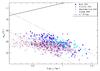 |
Fig. 1 Central brightness distribution of spiral disk in the samples of Kent (1985a), Courteau (1996), MacArthur et al. (2003) and Gadotti (2009). The two dashed lines corresponds to the limiting region containing spiral disks having absolute G magnitudes of −18 and −22 mag. The solid inclined line corresponds to the limiting surface brightness magnitude for object detection in the SM section, at a fiducial distance of 10 Mpc. Objects below that line have too low a central surface brightness to be detected by Gaia. As we can observe none of the observed pure exponential disks are in a state to be sampled by Gaia. |
In Fig. 1 we present an overview of the structural properties of the observed exponential disks derived from three selected samples extracted from the literature. The sample used by Kent (1985a) has 105 objects observed in the r band of the uvgr Thuan & Gunn (1976) system. The large majority of objects in this sample are spirals, and a few elliptical galaxies (11 objects) were also included. To bring these observations to the G photometric system of Gaia, we first transformed the data to the UBV Johnson-Cousin system using the equations quoted in Kent (1985b). Then we used a mean estimated colour B − V = 0.5 to convert the data to the G system using the transformations discussed in the previous section. The second sample was extracted from Courteau (1996) as derived from observations in the r Spinrad Lick filter, and we adopted the calibration quoted in the paper to match the system used by Kent (1985a) and then applied the same transformation used before to the G system. We also applied the same face-on correction adopted by Kent (1985a) to the Courteau (1996) data. The sample of MacArthur et al. (2003) was observed in the BVRH system, easing the transformation to the G system from the results directly observed in the V band. The data in Gadotti (2009) is composed of nearly 1000 galaxies extracted from the Sloan Digital Survey and analysed with the program BUDDA (de Souza et al. 2004) which is able to fit a bulge+disk+bar model directly to the observed images.
A first word of caution is needed because of the uncertainty in comparing the photometric systems used in these studies. Moreover, the process of deriving the disk structural parameters is also different. The analysis of Kent (1985a) was done through a fit of the minor and major axis brightness profiles to a combination of de Vaucouleurs r1/4 bulge plus an exponential disk profile. Courteau (1996) have adopted an elliptical approximation that describes the isophotal levels to obtain the major axis light profiles that were fitted to a composite model with an exponential disk plus an r1/4 bulge model. MacArthur et al. (2003) combined an exponential disk with a Sérsic r1 /n law to describe the bulges. Nevertheless, we can see from Fig. 1 that the spiral disks of these three samples consistently occupy approximately the same region of the μ0d − Log re diagram with a small offset probably due to a combination of the different approaches adopted to determine the structural parameters. The two traced predict an exponential disk having absolute G magnitude of −18 and −22, and we can see that they are approximately consistent with the observed trend of the empirical points as pointed out by Kent (1985a).
The continuous line in Fig. 1 corresponds to the SM detection limit G = 20 mag computed by assuming a fiducial distance of 10 Mpc representative of a close nearby spiral disk. For a given combination of the parameters μ0d and re(kpc), we correct for the distance effect in the pixel illumination and estimate the surface brightness distribution using Eq. (2). Then we use a numerical interpolation routine to divide each Gaia physical pixel into a 30 × 30 mesh to compute the total flux contribution per pixel. The estimated fluxes were evaluated as they will be observed in the 5 × 5 SM sample working windows by applying the VPA Gaia detection criteria presented in Sect. 1. We observe from the continuous line in Fig. 1 that the surface brightness detection limit is relatively close to our crude estimation presented at the end of the previous section for objects with small effective radius, but it also shows a consistent trend to be brighter for objects with large effective radius. This effect arises because a lower effective radius implies a steeper profile with a larger fraction of the disk flux concentrated in the central pixel, and as a consequence, the evaluated SM background becomes lower when compared with the central surface brightness of the galaxy. In contrast the light is more diffusely distributed in disks with larger effective radius, and only those objects with extremely high central surface brightness could be detected. We can further verify that the observed spiral disks in the local Universe showing the highest central surface brightness are located in the region μ0d(G) ≃ 18mag/□′′ well below the detection limit of the Gaia system.
We should also point out that by increasing the distance, the estimated apparent magnitude in a given SM working window of Gaia is also increased due to a combination effect of the background subtraction procedure and to the fixed size of each pixel requiring therefore higher levels of surface brightness to reach the stipulated detection limit. Therefore we are forced to conclude that the observations of the Gaia satellite will not be able to examine the properties of the spiral disks observed in the local universe. Even if we consider that the detected images by Gaia will be downloaded, including the surrounded pixels within a three magnitude level, only the very bright nearby disks will have any chance of being sampled. The only possible exception will be those objects having a bright non-stellar nuclei as an AGN and objects with strong nuclear star forming regions.
4. Spheroidal components
One of the most commonly adopted approximations to describe the luminosity distribution of spheroidal components, including bulges of spirals and elliptical galaxies, is the relation proposed by de Vaucouleurs (1948) ![Mathematical equation: \begin{equation} I(r)=I_{\rm e} \exp\left\lbrace-7.66925\left[\left(\frac{r}{r_{\rm e}}\right)^{1/4}-1 \right] \right\rbrace, \label{Eq08} \end{equation}](/articles/aa/full_html/2014/08/aa23514-14/aa23514-14-eq99.png) (8)where the constant k = 7.66925 is defined in such a way that re represent the effective radius containing half of the total luminosity, and Ie is the corresponding surface brightness at the effective radius. For obvious reasons this relation is also known as the r1/4 profile. As a consequence the central surface brightness of the spheroidal component is
(8)where the constant k = 7.66925 is defined in such a way that re represent the effective radius containing half of the total luminosity, and Ie is the corresponding surface brightness at the effective radius. For obvious reasons this relation is also known as the r1/4 profile. As a consequence the central surface brightness of the spheroidal component is  (9)or μ0 = μe − 8.327, indicating that for a given effective surface brightness, the spheroidal structure tends to present a much larger central surface brightness than the one observed in the exponential disks easing therefore its detection by Gaia. The total luminosity of the r1/4 profile derived from this expression is
  (10)where q = b/a represents the axial ratio of the adopted structure of concentric elliptical isophotal levels. The absolute magnitude derived for this profile is
  (11)where the effective radius is expressed in Kpc.
For some objects the r1/4 profile gives a good empirical representation of the data. But in several cases this profile is clearly not adequate for representing the whole dynamical range of the observed surface brightness distribution. In recent years a preference has been established to describe the spheroidal component by using the Sérsic (1969) 1 /n law, which is a generalization of de Vaucouleur’s law: ![Mathematical equation: \begin{equation} I(r)=I_{\rm e} \exp\left\lbrace -b_n\left[\left(\frac{r}{r_{\rm e}}\right)^{1/n}-1 \right] \right\rbrace. \label{Eq12} \end{equation}](/articles/aa/full_html/2014/08/aa23514-14/aa23514-14-eq107.png) (12)By adopting n = 4 the normalization constant becomes bn = 7.66925, and the Sérsic law reproduces de Vaucouleur’s law. For n< 4, the light distribution has a less concentrated profile. In particular when n = 1, the constant is bn = 1.67834699, and the profile is identical to the one used to describe the exponential disk. For n> 4 the Sérsic profile has a hard, highly concentrated brightness distribution. The constant bn is determined by the condition that re is the effective radius and Ie the surface brightness, and one useful approximation to evaluate this constant was derived by Ciotti & Bertin (1999):
(12)By adopting n = 4 the normalization constant becomes bn = 7.66925, and the Sérsic law reproduces de Vaucouleur’s law. For n< 4, the light distribution has a less concentrated profile. In particular when n = 1, the constant is bn = 1.67834699, and the profile is identical to the one used to describe the exponential disk. For n> 4 the Sérsic profile has a hard, highly concentrated brightness distribution. The constant bn is determined by the condition that re is the effective radius and Ie the surface brightness, and one useful approximation to evaluate this constant was derived by Ciotti & Bertin (1999): 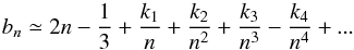 (13)where k1 = 4/405, k2 = 46/25 515, k3 = 131/1 148 175, and k4 = 2 194 697/30 690 717 750.
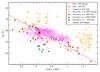 |
Fig. 2 Correlation between the effective brightness and effective radius observed in nearby spheroids. The orange circles and red triangles respectively represent the bulges and ellipticals from Kent (1985a). The red crosses are the Virgo cluster ellipticals from Caon et al. (1993). The orange diamonds are the bulge data from MacArthur et al. (2003). The red circles are the ellipticals from Kormendy et al. (2009). The small pink circles represent the sample of bulges studied by Gadotti (2009). The dashed line represents the Hamabe & Kormendy (1987) empirical relation. |
The central surface brightness of the Sérsic profile is  (14)indicating that μ0 = μe − 1.0857bn, and we can observe that the central surface brightness depends on the value adopted for the exponent n. In the regime n> 4, the central brightness becomes increasingly greater implying a brighter central region for a given effective brightness. The analogous relation for the asymptotic total luminosity is
  (15)From the image decomposition analysis of several objects the existence of a correlation emerges between the effective brightness and effective radius of elliptical and bulges generally known as the Kormendy relation (Hamabe & Kormendy 1987). This correlation, shown in Fig. 2, indicates that there is a fundamental link established during the formation process between the structural parameters describing the light distribution of spheroids:
  (16)Using the de Vaucouleur profile, we can observe that the Kormendy relation, together with Eqs. (11) or (15) for the corresponding Sérsic profile, implies that the more luminous objects are located in the extreme lower right-hand region of Fig. 2 therefore having a larger effective radius and also a lower effective surface brightness. In the analysis of Kent (1985a), it was adopted the de Vaucouleur’s law to describe the spheroidal component of bulges and ellipticals. The sample of spirals investigated by Kent are spread over all the morphological types, and several objects have S0-Sa early type morphology. The data from Caon et al. (1993) observations of 52 elliptical and S0 galaxies in the Virgo cluster was fitted with the Sérsic law. These authors have demonstrated that the r1 /n profile, with 1 <n< 15 give a more unbiased and accurate representation of the observed brightness profile. The vast majority of these objects have n = 3.8 ± 5 with no clear distinction between ellipticals and S0. The position of the bulges in the sample of MacArthur et al. (2003) have 121 spiral galaxies, most of which have morphological types later than Sb.
According to these authors, the adopted exponent of the bulge r1 /n profile is observed to be restricted to the region n< 3 peaked around n = 1 ± 0.4 close to the pure exponential solution. Therefore the light distribution of bulges in this late type sample is much less concentrated than the results found for S0 galaxies in Kent (1985a) and Caon et al. (1993). Moreover, spirals in the sample of MacArthur et al. (2003) tend to present a correlation between the bulge effective radius and the disk scale length ⟨ reb/rd ⟩ = 0.22 ± 0.09, indicating that the bulges of late type spirals are more affected by the presence of the stellar disk. The sample of bulges of spirals extracted from the SDSS and studied by Gadotti (2009) obeys approximately the same relation as observed in elliptical galaxies with a difference in the angular coefficient. Finally the sample of Kormendy et al. (2009) discuss the spheroidal objects with high HST resolution nuclear images. Their analysis indicate that 2 <n< 15 concentrated at n = 2 − 4 showing different behaviour between ellipticals and S0 in one hand and low luminosity spheroidal ellipticals. We observe that despite the difference in photometric resolution and analysis method there is a relatively good agreement between these samples in the description of the overall photometric properties of ellipticals and bulges.
The observed dispersion around the mean trend of the Kormendy relation is real and results from the fact that this relation can be interpreted as a projection of a deeper relationship describing the fundamental plane of spheroids (Djorgovski et al. 1996). One additional interesting feature that we can observe is that for a given effective radius, the surface effective brightness of bulges tends to be brighter than the corresponding elliptical. This trend is more evident in the samples of both Kent (1985a) and MacArthur et al. (2003) with the difference that the bulges of early type spirals seem to be smaller and brighter than the corresponding bulges of late type galaxies. However, in the sample of Gadotti (2009), where the photometric components are simultaneously derived from a direct fit of the image, this effect is subtler. Therefore it might be possible that the differences between the Kormendy relation in bulges and ellipticals is partially affected by the adopted process used to decompose the relative contributions of disks and bulges in spiral galaxies.
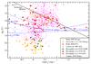 |
Fig. 3 Central brightness distribution versus effective radius of spheroids of the same data sources used in Fig. 2. The black line indicates the predicted position of brightness profiles obeying the Kormendy relation for an index n = 4 of the Sérsic profile. The vertical spread of the data is due to variations in the index n observed in the observed profiles. Objects with steeper profiles (n> 4) are located above that line, while objects with softer profiles (n< 4) populate the lower region. The blue lines correspond to the limiting surface brightness of Sérsic spheroids at a fiducial distance equal to 10 Mpc having G = 20 mag in the Gaia SM section. Objects located above the limiting line are able to be detected, and depending on the Sérsic index (n), the location of the limit of detection will be different. For n> 4 the predicted location of most objects, according to the Kormendy relation, is situated above the limiting curve and therefore they should be detected by Gaia. In contrast, spheroids having softer profiles, as shown in the sample of the MacArthur et al. (2003) bulges tend to be located below the Gaia detection limit and should not be detected. |
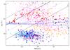 |
Fig. 4 Relation between the central brightness and absolute magnitude distribution for spheroids and stellar disks. The symbols are the same as in Figs. 1 and 2. Local stellar disks and bulges of late-type spirals are located below the Gaia detection limit for a fiducial distance of 10 Mpc and should not be detected. However, the vast majority of normal ellipticals and classical bulges have a sufficiently high central surface brightness to be detected. |
In Fig. 3 we present the spheroidal data in the μ0 × log re plane, which is more relevant in the discussion of Gaia observations. The predicted position of objects obeying the Kormendy relation for n = 4 brightness profiles approximately following the trend observed in the samples of Kent (1985a) and Caon et al. (1993). We can still observe, as mentioned in the discussion of Fig. 2, that for a fixed value of n, the larger and more luminous objects tend to present a lower central surface brightness along that line. The region above that line is populated by objects having a more steeper brightness profile with n> 4, while the lower region is richer in objects having softer (n< 4) profiles. A variation Δn = 1 in the index of the Sérsic profile will displace the position of the Kormendy relation by Δμ0 = 2.17 mag increasing the vertical spread seen in this diagram. Most of the bulges observed in the sample of late spirals of MacArthur et al. (2003) are located in the lower (n ≃ 1) region displaced by approximately 6.5 mag relative to the n = 4 Kormendy relation.
The lines corresponding to n = 2, 3, 4, and 5 in Fig. 3 represent the limiting surface brightness corresponding to the VPA detection criteria adopted by the Gaia Sky Mapper to identify a G = 20 mag object located at a fiducial distance d = 10 Mpc using the same numerical integration routine as explained in Sect. 2. At that distance we observe that for n> 2 most of the normal spheroids, including a large fraction of bulges, are located in the detection region of the Gaia satellite with the possible exception of a few large and bright objects. For n< 2 the observed central brightness is lower, and considering the additional difficulty due to the background subtraction it turns out that a larger number of bulges and ellipticals having soft brightness profiles tend to escape the limit of detection. In particular, the bulges of late spirals observed by MacArthur et al. (2003) and some of the spheroidal galaxies in the sample of Kormendy et al. (2009) and ellipticals with n< 2 quite probably will not be detected by Gaia. Nevertheless, we observe from the large homogeneous sample of Gadotti (2009), representative of the whole distribution of morphological types, that Gaia should be able to observe a large number of local bulges that have relatively steeper brightness profiles.
Another point of concern is that the extrapolation of the Sérsic profile to the central region below 1 arcsec indicates some extremely high central surface brightness that is not realistic. This effect has already been recognized by Caon et al. (1993) and confirmed from data of the HST high resolution images of Kormendy et al. (2009), among others. In their very central regions, ellipticals show a dichotomy with some objects presenting an inner core where the surface brightness is lower than predicted by the Sérsic profile. In other objects the observed profile shows cuspy behaviour where the surface brightness is significantly higher than the Sérsic profile. According to Kormendy et al. (2009), there is a trend in that bright ellipticals tend to show a core profile, while lower luminosity objects with −21.54 <MV< − 15.53 tend to present an extra light cuspy central region. Moreover, no object exists in this whole sample with a central surface brightness in excess of 10mag/□′′. Therefore the very high brightness inferred from n> 4 profiles should be treated with caution. In fact we could expect that the observations of Gaia should be of great help in clarifying this effect by the observation of a large number of objects.
The detection limit imposed by Gaia can also be examined using all objects, including disks and spheroids, in a plot of the central surface brightness against the total absolute magnitude of each component as presented in Fig. 4. In this diagram the disks of spiral galaxies are clearly segregated to a relatively small region well below the detection limit of Gaia as we have already concluded. Directly above this region, we can see the broad inclined strip domain occupied by elliptical galaxies having a Sérsic exponent in the interval n = 3 − 5. The black lines indicate the predicted locus of spheroidal components obeying the Kormendy relation. The blue lines correspond to the same Gaia limiting region for detection in the SM section at the fiducial distance of 10 Mpc seen in Fig. 3. Objects above that line are able to be detected by Gaia. We observe that objects similar to the bright luminous elliptical galaxies with MG> − 22 studied by Kormendy et al. (2009) and having high definition images from HST should be located close to Gaia’s detection limit. As mentioned before, those very bright ellipticals tend to present a larger effective radius, and as a consequence of the Kormendy relation, their effective surface brightness is lower, as is their central surface brightness. Except for these few very luminous objects the vast majority of ellipticals are located well inside the detection region of Gaia. The situation of bulges is less clear. The bulges of early type spirals observed by Kent (1985a) and the few S0 objects studied by Kormendy et al. (2009) are consistently close to the region occupied by ellipticals also inside the detection limit of Gaia. However a large fraction of the bulges of late type spirals in the sample of MacArthur et al. (2003) have softer brightness profile with n< 2 and are well below the limit of detection. The same situation is observed in the case of some spheroidal ellipticals that should escape to Gaia detection. In the sample of Gadotti (2009) we see that only those low luminosity bulges with low surface central surface brightness will escape detection, but the vast majority of normal bulges are well inside the detection region.
5. Numerical simulations
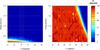 |
Fig. 5 Efficiency detection maps of simulated brightness profiles at the Sky Mappers produced by the Gaia VPA Prototype implemented in GIBIS. On the left, exponential profiles. On the right, de Vaucouleurs profiles. |
An exact scenario of the detections of extended objects by Gaia will only be available after the first months of the mission, during a phase called initial in orbit calibration. At that phase, the satellite will continuously observe a region around the ecliptic pole, and thus the physical characteristics of the objects detected and transmitted to the Earth may be determined. However, to assess whether the scenario described in this paper is supported by the prototype of the on-board video-processing algorithm, we can already compare results from realistic simulations of the instrument.
To do so, we performed fully numerical simulations of galaxy images in the Gaia focal plane and of their detection. These simulations adopted the Gaia Instrument and Basic Image Simulator, or GIBIS (Babusiaux et al. 2005, 2011), and the on-board video processing-algorithm prototype implemented in this simulator.
The simulations were performed towards the (l,b)gal = (40.0°,52.0°) direction. These coordinates were chosen for statistical reasons, since the GIBIS scanning law predicts a large number of observations around it. Because the simulated profiles are symmetric, any other positions on the sky present similar results, with statistical fluctuation depending on the number of transits. The simulations spanned a parameter space covering disk and bulge radii between 0.2′′ and 2.0′′ and integrated V magnitudes from G = 14 to G = 20, regardless of their physical relevance. All simulated objects were symmetric, and 10 000 synthetic objects were generated representing two extreme types: pure bulge brightness profiles following the de Vaucouleurs law (n = 4) and pure disk profiles following an exponential law.
The parameters adopted for the detection algorithms were the nominal ones, so may change after an optimization campaign. Even though optimized parameters may improve the detection of extended objects a little, significant deviations from the results presented herein are not expected.
In Fig. 5 we present the resulting sky mapper detection maps for each type of object. The colour map encodes detection efficiency at each each region of the integrated magnitude vs. radius plane. This was computed as the fraction of the total simulated transits in which the objects that lie at that position of the parameter space were detected. The results presented in this figure indicate that while most de Vaucouleurs profiles were detected, there is a large detection valley amongst the exponential profiles. The small scale variations that can be seen in all these maps are artefacts created by the simulated Gaia scanning law and the CCD gaps in the focal plane; accordingly, they change randomly depending on the sky direction in which the simulation is performed.
The main conclusion obtained from this test is that galaxies dominated by a disk component are expected to be very poorly detected at the sky mapper level, and thus will probably not be confirmed further by at the astrometric field level and not be transmitted to the ground. In contrast, most galaxies with prominent de Vaucouleurs-like bulges, or elliptical galaxies, will be detected and thus probably transmitted. This corroborates the conclusions obtained in the previous sections of this work.
6. Distance effect
Even if they are close enough to be not affected by a large amount of cosmic evolution and therefore have exactly the same nuclear surface brightness as the z = 0 objects, the Gaia observations of more distant objects will be modified by two major effects. First, there is a contribution of the cosmological dimming on the surface brightness due to the Tolman effect implying that I0(z) = I0/ (1 + z)4. Second, there is a geometric dilution effect since a larger spatial region will be sampled in the fixed angular size of the Gaia pixel.
The result of the combination of these effects is that the corresponding average central surface brightness of the objects in the SM working windows becomes progressively fainter as we increase the distance. We consider as an example a typical relatively bright elliptical galaxy with n = 4 and log re(kpc) = 0.5 having an effective surface brightness μe = 21.33mag/□′′ at z = 0 and Mabs = −21.13 by the Kormendy relation. At a distance of 10 Mpc, its central surface brightness is 13.02 mag/□′′, which is almost identical to the corresponding value at z = 0. At that distance we estimate, by numerical integration of the Sérsic profile, that the detected magnitude of this object in the central sample of the SM detection window will be 18.03 mag while the background is 19.18 mag. After adding the counts in the 3 × 3 SM window, and correcting for the background contribution and the Gaia PSF adopted correction, we conclude that the estimated total magnitude equals to G = 16.73 mag and therefore the object will be easily detected. However, using the cosmological concordance model (H0 = 70km s-1 Mpc-1, Ωm = 0.27, ΩΛ = 0.73) to estimate the redshift, this same object when located at 600 Mpc will have an average central surface brightness of 13.58 mag/□′′, and now the magnitude in the central sample of the SM section will be 21.20 mag, while the background contribution per sample is 24.57 mag. At that distance the total corrected magnitude in the SM window will be G = 19.99 mag practically equal to the stipulated limiting Gaia magnitude.
One consequence of this effect is that an increasingly larger proportion of objects leave the detection region as the distance is increased and practically no objects with n = 4 should be detected beyond 600 Mpc. This effect is shown in Fig. 6 where we estimate the variation in the mean surface brightness of the detectable objects integrated in the SM central pixel of Gaia, in the euclidean approximation, as we observe objects at higher distance. The three panels illustrate the effect suffered by elliptical galaxies described by Sérsic profiles with n = 3, 4, and 5. Each diagram indicates the predicted behaviour of detected spheroids, including almost the entire population of elliptical galaxies with effective radius in the interval between log re(kpc) = −0.5 and 1.5 and obeying the observed local Kormendy relation. The two extreme effective radii defining this region were chosen to comprise the vast majority of ellipticals in the local Universe. The variation in the Gaia detection limit, G = 20 mag in the SM section, is indicated in the plane of the surface brightness versus increasing distance for objects satisfying the Kormendy relation.
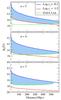 |
Fig. 6 Effect of distance in the mean surface brightness of the central pixel of Gaia of elliptical galaxies described by Sérsic profile. The blue and red lines correspond to the size limits log re(kpc) = −0.5 and log re(kpc) = 1.5 comprising the vast majority of known ellipticals with good profile decomposition. |
When n = 4 the expectation is that even the population of ellipticals with larger effective radius, hence lower surface brightness and high total absolute magnitude, should be detected by Gaia up to a distance around 170 Mpc. Above this limit we begin to lose a progressively higher fraction of ellipticals having larger effective radius. Objects with smaller effective radius tend to present higher central surface brightness and should be detected at greater distances in this nearby cosmic neighbourhood. But as the distance increases to a limit of the order of 610 Mpc, all the n = 4 elliptical population is lost due to the increasing contribution of the geometric distance dilution and the dimming from the Tolman effect, which is responsible for an increase of 0.57mag/□′′ in the central surface brightness. Also indicated is the fraction of the population that will have a chance of being detected at each distance.
An exact estimation of the extent of this effect is a hard task, since we do not know exactly how real objects described by a given n Sérsic profile are spread out over the effective radius interval, and moreover, there is no guarantee that the Sérsic profile could be a good description of the surface brightness in the galactic central region. The number of local objects having good photometric decomposition structure parameters is relatively small and the cosmic distribution of the effective radius amongst ellipticals is not precisely known. Judging from Fig. 3 and from the homogeneous data of Caon et al. (1993) and Kormendy et al. (2009), we roughly estimate that observed objects are restricted to the indicated interval −0.5 < log re(kpc) < 1.5.
If we go on to make the arbitrary assumption that these objects are evenly spread inside this interval, we can estimate that the extent of the shaded region is indicative of the fraction of observable objects. Using this crude approximation we estimate that most of the available population of ellipticals presenting an n = 4 profile will be observed up to a distance of 170 Mpc and approximately one third of the objects between 170 Mpc and 600 Mpc should be lost. Beyond that distance corresponding to z = 0.14, the n = 4 ellipticals should barely be observable by Gaia.
In the case of an n = 5 profile presented in the superior panel of Fig. 6, the indication is that the entire population of the bright nuclear elliptical will be observed in our neighbourhood. The situation for objects with soft n = 3 profiles is more severely limited, since even in our close vicinity, only 50% of them have any chance of being detected.
One interesting quantity to obtain is the total number of probable objects to be observed. Admitting that most of the elliptical galaxies can be represented by the n = 4 profile, we can estimate the total number of objects in each distance interval. According to de Bernardi et al. (2010), the local density number of ellipticals from the SDSS survey is estimated as 10-3 gal/Mpc3. Therefore we can loosely conclude that the total number of detection by Gaia, corrected by the Milk Way zone of avoidance, should be of the order of 19 000 objects classified as elliptical up to 170 Mpc. Using these numbers we can further estimate that in the distance interval 170−600 Mpc, Gaia should detect half a million elliptical galaxies.
The situation of bulges is even less clear than the case of ellipticals. Quite probably the bulges of late type spirals will be difficult to detect owing to their soft brightness profile. The best hope of detecting bulges lies in the early-type spirals of S0-Sa morphological classes where a class of r1/4 spheroids are more commonly observed. Based on morphologically classified objects of the SDSS survey, Nakamura et al. (2003) conclude that the density of early-type galaxies (E + S0) is of the order of 1.7 × 10⁻³ gal/Mpc3 for H0 = 70 km s-1 Mpc-1. Therefore, we might expect that the number of Gaia detections could be approximately doubled by including the bulges of early-type spiral galaxies.
7. Conclusions
Based on the present status of Gaia mission our main conclusions are:
-
It is quite unlikely that the stellar disks could be detected except ifwe consider the population of objects harbouring AGNs andthose presenting strong nuclear star forming episodes.
-
The major fraction of detections will quite probably be constituted by normal ellipticals and bulges of S0-Sb galaxies that have steeper brightness profiles and Sérsic indices n = 3 − 5 or larger. A crude estimate indicates that the possible number of elliptical detections in the nearby 170 Mpc is situated around 19 000 objects and could be doubled by including of S0-Sa bulges. The population of very bright ellipticals present a relatively lower central surface brightness, and some of them could escape detection.
-
More distant objects, in the range 170−600 Mpc, could be observed but the evaluation of the total number of possible detections is more uncertain. If most of the population is represented by a Sérsic profile n = 4, then about two thirds of them could be detected increasing the total number of sources to half a million objects.
-
Ellipticals having soft brightness profiles, n< 3, will be more difficult to detect, and the same is valid for spheroidal galaxies.
-
This scenario is supported by numerical simulations of the detection at the sky mapper level. These simulations were performed by the Gaia Instrument and Basic Image Simulation and the video processing algorithm prototype using nominal parameters.
In the past ellipticals were considered relaxed systems that evolved passively due to little or no gas reservoir, formed from a monolithic collapse scenario, in a single burst of intense star formation. Nowadays, this picture has completely changed owing to recent photometric and kinematic studies that have revealed huge complexity in their dynamical structure, star formation history, and assembly history. These studies have been showing that ellipticals can be classified in three groups according with their luminosity. The photometric and kinematic properties of each group are very different and depend on their luminosity (Mo et al. 2010; Blanton & Moustakas 2009). Therefore the high resolution Gaia observations in the central region of ellipticals could be very useful for testing these different scenarios by using a homogeneous sample of objects.
A large fraction of the observed sample of nearby galaxies brighter than GRVS = 17 mag should also be detected in the spectrophotometer and due to its characteristics, the same object will be observed several times in different angle directions. Another interesting subject is that the detected objects should also be observed in the blue (BP) and red (RP) photometers. This would be an invaluable information for the stellar population studies in the central regions of galaxies.
One interesting issue is the discussion of the scientific impact of changing the limiting detection magnitude of Gaia to G = 21 mag. Such a change will obviously affect the quantity of data processing and is a matter under discussion by the mission control board. If this change could be consolidated, we might ask about its impact on the detection of galaxies. In the case of the disks, it is conceivable that this change will not modify the scenario discussed in Sect. 3. As we can see from Fig. 1, a variation of one magnitude on the detection limit magnitude
will not be able to include the population of normal stellar disks. On the other hand, that change will include a significant higher fraction of local spheroids as we can observe from Fig. 3. Perhaps more importantly, it will include a fraction of local spheroids with soft surface brightness profiles similar to those found in some of the local spheroidal ellipticals, as well as a fraction of the spheroidal bulges of late spirals observed by MacArthur et al. (2003). In the case of normal n = 4 ellipticals, the upgrade to G = 21 mag will include a large fraction of the objects that are more distant than 170 Mpc in the detection list. If we consider an object with log re(kpc) = 1.5 obeying the Kormendy relation, which therefore corresponds to a very luminous elliptical with Mabs = −23.19 mag, it will have at d = 600 Mpc a total corrected magnitude in the SM window of G = 21.00 mag and therefore will be included in the list of detected objects. Therefore the limiting distance for completion will triple expanding our number of estimated detection approximately by a factor of 30.
Acknowledgments
Part of this work was partially supported by CAPES/ COFECUB and by the Portuguese agency FCT (SFRH/BPD/74697/2010, PTDC/CTE-SPA/118692/2010). We also thank the French CNES for providing computational resources, and the Gaia Data Processing and Analysis Consortium Coordination Unit 2 – Simulations for the Gaia Instrument and Basic Image Simulator. We also acknowledge Jos de Bruijne for kindly providing information regarding the functioning of the onboard VPA detection software. We also thanks an anonymous referee for the helpful comments.
References
- Babusiaux, C. 2005, in The Three-Dimensional Universe with Gaia, eds. C. Turon, K. S. O’Flaherty, & M. A. C. Perryman, ESA SP, 576, 417 [Google Scholar]
- Babusiaux, C., Sartoretti, P., Leclerc, N., & Chéreau, F. 2011, Astrophysics Source Code Library, 7002 [Google Scholar]
- Bernardi, M., Shankar, F., Hyde, J. B., et al. 2010, MNRAS, 404, 2087 [NASA ADS] [Google Scholar]
- Blanton, M. R., & Moustakas, J. 2009, ARA&A, 47,159 [NASA ADS] [CrossRef] [Google Scholar]
- Caon, N., Capaccioli, M., & D’Onofrio, M., 1993, MNRAS, 265, 1013 [NASA ADS] [CrossRef] [Google Scholar]
- Ciotti, L., & Bertin, G., 1999, A&A, 352, 447 [NASA ADS] [Google Scholar]
- Courteau, S. 1996 , ApJS, 103, 363 [Google Scholar]
- de Bruijne, J. H. J., Allen, M., Prod’homme, M. , Krone-Martins, A., & Azaz, S. 2014, A&A, submitted [Google Scholar]
- de Souza, R. E., Gadotti, D. A., & dos Anjos, S. 2004, ApJS, 153, 411. [NASA ADS] [CrossRef] [Google Scholar]
- de Vaucouleurs, G. 1948, Ann. Astrophys., 11, 247 [Google Scholar]
- Djorgovski, S. G., Pahre, M. A., & de Carvalho, R. R. 1996, ASP Conf. Ser., 86, 129 [NASA ADS] [Google Scholar]
- Dollet, C., Bijaoui, A., & Mignard, F. 2005, Proc. of the Gaia Symp. The Three-Dimensional Universe with Gaia, ESA SP, 576, 429 [NASA ADS] [Google Scholar]
- Freeman, K. C. 1970, ApJ, 170, 811 [NASA ADS] [CrossRef] [Google Scholar]
- Gadotti, D. 2009, MNRAS, 393, 1531 [NASA ADS] [CrossRef] [Google Scholar]
- Hamabe, M., & Kormendy, J. 1987, Proc. IAU Symp., 127, 379 [Google Scholar]
- Harrison, D. L. 2011, Exp. Astron., 31, 157 [NASA ADS] [CrossRef] [Google Scholar]
- Jordi, C., Gebran, M., Carrasco, J. M., et al. 2010, A&A, 523, A48 [NASA ADS] [CrossRef] [EDP Sciences] [Google Scholar]
- Katz, D., Cropper, M., Meynadier, F., et al. 2010, EAS Pub. Ser., 45, 189 [Google Scholar]
- Kent, S. M. 1985a, ApJS, 59,115 [NASA ADS] [CrossRef] [Google Scholar]
- Kent, S. M. 1985b, PASP, 97, 165 [NASA ADS] [CrossRef] [Google Scholar]
- Kormendy, J., Fisher, D. B., Cornell, M. E., & Bender, R., 2009, ApJS, 182, 216 [NASA ADS] [CrossRef] [Google Scholar]
- Krone-Martins, A., Ducourant, C., Teixeira, R., et al. 2013, A&A, 556, A102 [NASA ADS] [CrossRef] [EDP Sciences] [Google Scholar]
- MacArthur, L. A., Courteau, S., & Holtzman, J. A., 2003, ApJ, 582, 689 [NASA ADS] [CrossRef] [Google Scholar]
- Mo, H., van den Bosch, F., & White, S. 2010, in Galaxy Formation and Evolution (Cambridge University Press) [Google Scholar]
- Nakamura, O., Fukujita, M., Yasuda, N., et al. 2003, AJ, 125, 1682 [NASA ADS] [CrossRef] [Google Scholar]
- Perryman, M. A. C., de Boer, K. S., Gilmore, G., et al. 2001, A&A, 369, 339 [NASA ADS] [CrossRef] [EDP Sciences] [Google Scholar]
- Provost, S., Le Roy, M., Mamdy, B., Flandin, G., & Paulsen, T. 2007, Proc. of DASIA 2007 – Data Systems In Aerospace, ed. by L. Ouwehand. ESA SP, 638, 39 [Google Scholar]
- Roberts, M. S., & Haynes, M. P. 1994, ARA&A, 32, 115 [NASA ADS] [CrossRef] [Google Scholar]
- Robin, A.C., Luri, X., Reyl, C., et al. 2012, A&A, 543, A100 [NASA ADS] [CrossRef] [EDP Sciences] [Google Scholar]
- Sérsic, J. L. 1969, Atlas de Galaxias Australes (Cordoba: Observatorio Astronomico) [Google Scholar]
- Thuan, T. X., & Gunn, J. E., 1976, PASP, 88, 543 [NASA ADS] [CrossRef] [Google Scholar]
All Figures
|
Fig. 1 Central brightness distribution of spiral disk in the samples of Kent (1985a), Courteau (1996), MacArthur et al. (2003) and Gadotti (2009). The two dashed lines corresponds to the limiting region containing spiral disks having absolute G magnitudes of −18 and −22 mag. The solid inclined line corresponds to the limiting surface brightness magnitude for object detection in the SM section, at a fiducial distance of 10 Mpc. Objects below that line have too low a central surface brightness to be detected by Gaia. As we can observe none of the observed pure exponential disks are in a state to be sampled by Gaia. |
| In the text | |
|
Fig. 2 Correlation between the effective brightness and effective radius observed in nearby spheroids. The orange circles and red triangles respectively represent the bulges and ellipticals from Kent (1985a). The red crosses are the Virgo cluster ellipticals from Caon et al. (1993). The orange diamonds are the bulge data from MacArthur et al. (2003). The red circles are the ellipticals from Kormendy et al. (2009). The small pink circles represent the sample of bulges studied by Gadotti (2009). The dashed line represents the Hamabe & Kormendy (1987) empirical relation. |
| In the text | |
|
Fig. 3 Central brightness distribution versus effective radius of spheroids of the same data sources used in Fig. 2. The black line indicates the predicted position of brightness profiles obeying the Kormendy relation for an index n = 4 of the Sérsic profile. The vertical spread of the data is due to variations in the index n observed in the observed profiles. Objects with steeper profiles (n> 4) are located above that line, while objects with softer profiles (n< 4) populate the lower region. The blue lines correspond to the limiting surface brightness of Sérsic spheroids at a fiducial distance equal to 10 Mpc having G = 20 mag in the Gaia SM section. Objects located above the limiting line are able to be detected, and depending on the Sérsic index (n), the location of the limit of detection will be different. For n> 4 the predicted location of most objects, according to the Kormendy relation, is situated above the limiting curve and therefore they should be detected by Gaia. In contrast, spheroids having softer profiles, as shown in the sample of the MacArthur et al. (2003) bulges tend to be located below the Gaia detection limit and should not be detected. |
| In the text | |
|
Fig. 4 Relation between the central brightness and absolute magnitude distribution for spheroids and stellar disks. The symbols are the same as in Figs. 1 and 2. Local stellar disks and bulges of late-type spirals are located below the Gaia detection limit for a fiducial distance of 10 Mpc and should not be detected. However, the vast majority of normal ellipticals and classical bulges have a sufficiently high central surface brightness to be detected. |
| In the text | |
|
Fig. 5 Efficiency detection maps of simulated brightness profiles at the Sky Mappers produced by the Gaia VPA Prototype implemented in GIBIS. On the left, exponential profiles. On the right, de Vaucouleurs profiles. |
| In the text | |
|
Fig. 6 Effect of distance in the mean surface brightness of the central pixel of Gaia of elliptical galaxies described by Sérsic profile. The blue and red lines correspond to the size limits log re(kpc) = −0.5 and log re(kpc) = 1.5 comprising the vast majority of known ellipticals with good profile decomposition. |
| In the text | |
Current usage metrics show cumulative count of Article Views (full-text article views including HTML views, PDF and ePub downloads, according to the available data) and Abstracts Views on Vision4Press platform.
Data correspond to usage on the plateform after 2015. The current usage metrics is available 48-96 hours after online publication and is updated daily on week days.
Initial download of the metrics may take a while.