© ESO, 2014

1. Introduction

Every high-resolution technique at optical-infrared wavelengths suffers from atmospheric turbulence, causing piston and tip tilt variations in the stellar light beams. For interferometric observations, any fluctuation, particularly in the optical path difference (OPD), leads to a degradation of the fringe power, hence a jitter in the fringe visibility. To overcome these problems, the various disturbances have to be corrected on a time scale of milliseconds – depending on the observed wavelength.

For interferometry such a correction usually implies using an external fringe tracker that sends offsets to a delay line in real time. Ideally, this will lead to a stable (with respect to variations in the fringe position) interferogram on the beam combiner used for the scientific observation. Besides an increase in data quality (stability of correlated flux measurements), an increase in sensitivity without extended integration time can be observed. At the ESO Very Large Telescope Interferometer (VLTI, Haguenauer et al. 2012), we set this up for the MID-infrared Interferometric instrument (MIDI Leinert et al. 2003) where the PRIMA FSU-A is used as an external fringe tracker, the so-called MIDI+FSU-A mode (Müller et al. 2010; Pott et al. 2012).

MIDI is a two-beam Michelson type interferometer, which operates in the N band, and produces spectrally dispersed fringe packages between 8 μm and 13 μm. The instrument is usually operated with a prism as dispersive element, providing a resolution of R ≈ 30. Given the wavelength range, MIDI is suited to observations of objects with dusty environments, especially young stellar objects (YSO, e.g., van Boekel et al. 2004; Ratzka et al. 2009; Olofsson et al. 2013; Boley et al. 2013) surrounded by circumstellar envelopes and protoplanetary disks and active galactic nuclei (AGN, e.g., Jaffe et al. 2004; Burtscher et al. 2013). Since 2004 the MIDI instrument has been available to the astronomical community and become one of the most prolific interferometric instruments to date with more than 100 scientific publications in refereed journals.

The new facility at VLTI for phase-referenced imaging and micro-arcsecond astrometry (PRIMA, Delplancke 2008; van Belle et al. 2008) is currently undergoing its commissioning phase. PRIMA consists of four subsystems: the star-separator module (STS, Nijenhuis et al. 2008), the internal laser metrology (Schuhler 2007), the differential delay lines (DDL, Pepe et al. 2008), and two identical fringe sensor units (called FSU-A and FSU-B). However, for the MIDI+FSU-A mode alone, the FSU-A from the PRIMA subsystems is relevant. A detailed description of the FSUs is given by Sahlmann et al. 2009. We briefly summarize the principle setup of the FSU-A:

• The FSU-A operates in the K band between 2.0 μm and 2.5 μm.

• Polarizing beam splitters separate the p and s components of the individual beams, resulting in four beams separated by 90°in phase, before they are injected into single-mode fibers.

• The fibers send the light inside a cryostat where each of the four beams gets dispersed by a prism over five pixels on one quadrant of a detector.

• For each quadrant a synthetic white light pixel is computed by summing up the flux measured by the five spectral pixels.

Given the setup, the four light beams are phase-shifted spatially. The intensity of a sinusoidal signal (or fringe package) is therefore measured at four points separated by a quarter of a wavelength. This so-called ABCD principle allows computation of the fringe phase and group delay, as well as visibility directly (see Eqs. (4) and (5) in Shao & Staelin 1977) and in real time.

In this paper, the operation scheme of the MIDI+FSU-A mode is briefly described in Sect. 2. The performance of this new mode and the measurement of K band visibilities are presented in Sects. 3 and 4, respectively. Discussion and conclusions can be found in Sect. 5.

In the next paper of this series, we will discuss the achievable differential phase precision in the MIDI+FSU mode in detail, which is significantly improved by factors of 10–100 over the MIDI stand-alone operation thanks to the synchronous FSU tracking information. This new capability will be discussed in the context of faint companion detections down to the planetary regime.

2. Operating MIDI+FSU-A

The MIDI+FSU-A mode was made available to the community in April 2013 (ESO period 91), already. Therefore, it is part of a standardized observing scheme using observing templates, allowing efficient observations. Night operations at VLT/I consist of executions of observing blocks (OB) that are made of templates. Each template is tuned to a particular observation by setting its parameters called “keywords” (Peron & Grosbol 1997). The degree of complexity of the new acquisition template compared to the MIDI acquisition template increased only slightly with respect to available instrument parameters. The new keywords include flags for FSU-A sky calibration, operation frequency, and setups for fringe search and fringe scanning. The observing template has no new keywords.

2.1. VLTI setup

The MIDI+FSU-A mode can be operated with two 8.2 m unit telescopes (UT) or two 1.8 m auxiliary telescopes (AT). The light beams of the two telescopes are sent to a tunnel with delay lines (DL) to equalize the light paths of the two telescopes. After the beams enter the VLTI laboratory, a dichroic plate transmits the N band to MIDI while the near-infrared part of the light is transmitted to the other subsystems. Another dichroic plate sends the H-band to the IRIS (Infra-Red Image Sensor) tip-tilt corrector (Gitton et al. 2004), while the remaining K band is transmitted into the FSU-A. During observations, OPD corrections are sent through the optical path difference controller (OPDC) of the VLTI, which sends offsets to the VLTI delay lines. MIDI therefore only acts as cold camera. Fringe tracking by FSU-A and observations by MIDI occur on the same target, i.e. on-axis.

2.2. Observation sequence

In this section we describe a typical observation from a user’s point of view with its individual steps.

• Presetting (slewing) of the telescopes and delay lines, start of telescope, and IRIS “lab guiding” (VLTI tunnel and laboratory tip/tilt control); duration ≈3 min.

• Optional (mostly on the first target of the night that uses a given baseline): check of telescope pupil alignment and beam alignment in MIDI; duration ≈10 min.

• Optimization of flux injection into FSU-A using a beam tracking algorithm; duration ≈3 min.

• Record of sky background and flat fields for FSU-A; duration ≈3 min.

• Optional: Fringe search by driving a ramp with the main DL of typically ±1 cm to measure the zero OPD offset; duration ≈1 min.

• Optional: Fringe scanning through the fringe package for typically 250 times; duration ≈4 min.

• Initialization of fringe-tracking and MIDI+FSU-A data recording; duration typically ≈3 min.

If the optical paths are well aligned at the beginning of the night, a pure calibrator–science–calibrator observing sequence can be carried out typically in 30 min, making the MIDI+FSU-A mode into an efficient instrument even with its increased complexity. For detailed explanations about the PRIMA FSU fringe-tracking concept, we refer the interested reader to Sahlmann et al. (2010) and Schmid et al. (2012).

3. MIDI+FSU-A performance

The N band covers a range from 8 μm to 13 μm. This corresponds to a blackbody radiating with its highest flux density at roughly room temperature (≈300 K). Therefore, MIDI is dominated by a large thermal background stemming from sky emission, as well as of approximately two dozen mirrors in the light path between the source and the beam combiner. Because the scientific sources on sky are fainter by at least three orders of magnitudes with respect to the thermal background, one cannot simply use longer integration times as in the optical spectral regime. Otherwise, the detector would saturate. There is therefore a natural sensitivity limit for sources that can be detected by MIDI alone, which does not depend on the detector characteristics (except for its full well capacity and the size of the telescope’s primary mirror). In addition, atmospheric piston turbulence decreases the ability to reliably extract the interferometric signal in post-processing. Using an external fringe tracker, such as the FSU-A, provides additional information about the presence (in case the fringe-tracking loop is locked) and position (extrapolation form K band) of a fringe package, which can be used for the later reduction process. In the following, we both present several characteristics of the MIDI+FSU-A mode and highlight unmatched achievements.

In Fig. 1 we show a section of a so-called “waterfall” plot¹ of two typical MIDI observations taken without (Fig. 1a) and with (Fig. 1b) the FSU-A as external fringe tracker. The observations were performed on the same star (HD 187642, Altair) during the first MIDI+FSU-A test in the night of July 23, 2009, and were separated by 90 min (i.e., observed under almost the same conditions). In Fig. 1a the variations introduced by atmospheric piston fluctuations during the course of the MIDI observation can be clearly identified. The residuals in group delay (GD) are on the order of 11 μm. Using the external fringe tracker the N band signal is stabilized well (Fig. 1b) and atmospheric piston variations are corrected well by FSU-A.

Fig. 1 Waterfall plot of MIDI observations without (upper plot) and with FSU-A (lower plot) as an external fringe tracker. The horizontal axis can be interpreted as time, the vertical axis as OPD. Both plots display 2.5 min of observations.

Fig. 2 FSU-A group delay residuals as a function of K band magnitude (upper left), seeing (upper right), airmass (lower left), and coherence time (lower right).

A requirement for an external fringe tracker is the ability to correct for OPD variations caused by a turbulent atmosphere in real time; i.e., corrections have to be sent to the delay lines that are not slower than the current coherence time τ₀ of the atmosphere. The average value for the coherence time at Paranal is τ₀ = 3.9 ms in the visible spectral range at 500 nm (e.g., Sarazin & Tokovinin 2002). Therefore, an external fringe tracker has to operate in the kilo-Hertz regime with low latency on the order 1 ms. In the nights of November 29 to 31 in 2011 we observed various objects and calibrator stars (43 observations in total, see Table 1 for the observing log) during the course of the guaranteed time observations under program ID 087.C-0824. The observations were carried out under various conditions and allow a first assessment of the fringe-tracking performance. Figure 2 shows the measured FSU-A group delay residuals as a function of K band magnitude, seeing, airmass, and coherence time. For each subplot the linear correlation coefficient r and the probability p, which indicates whether the measured correlation can be generated by a random distribution (Bevington & Robinson 2003). The FSU-A performs well for the range of K band magnitudes explored here based on our requirements of what we consider a useful data set. This has a lock ratio of at least 30% and group delay residuals of less than λ_{N - band}/10, which is fulfilled for the majority of the data sets. A clear positive correlation can be identified for seeing, and a negative correlation for the coherence time. This can be explained by differential flux injection into the ABCD fibers. Under degraded atmospheric conditions, flux dropouts will result in low signal-to-noise ratio (S/N) values. For low target altitudes, i.e. higher airmass, a trend is at least visible, which might be explained by the increased amount of turbulent atmospheric layers the light has to pass. Also, longitudinal dispersion increases, leading to a lower fringe contrast. A longitudinal atmospheric dispersion compensator (LADC) is present for the FSU-A (Sahlmann et al. 2009) but is not tested and considered here. In Fig. 3 we show plots for the FSU-A lock ratio as a function of the parameters as in Fig. 2. The lock ratio is defined as the number of frames with the fringe-tracking loop closed divided by the total number of frames expressed in percent. Correlations are less prominent but still reflect the general picture that the fringe-tracking performance decreases under degraded atmospheric conditions and low object altitude.

Fig. 3 Same as Fig. 2 but for the FSU-A lock ratio.

3.1. Data reduction

The data reduction of bright N band targets (N ≳ 5 Jy using the ATs) observed with the MIDI+FSU-A mode can be carried out using the standard data reduction routines of EWS² (Jaffe 2004) and will not be explained further. For resolved or faint targets (N ≲ 5 Jy using the ATs), a different approach has to be chosen to reliably identify the MIDI interferograms and to measure the correlated fluxes. The K band data of the FSU-A carry the information directly about whether at any given time a fringe was observed or not based on the status of the OPDC. Therefore, N band data that are not directly visible in real time during the observation can be identified in post-processing by taking the FSU-A data into account. Using the HIGH_SENS mode of MIDI (all light of the target is sent directly to the N band beam combiner without recording photometry simultaneously), the integration time of one frame is 18 ms. The FSU-A is usually operated with 1 kHz leading to 18 FSU-A frames during one MIDI exposure. In a first step, the corresponding FSU-A frames for the individual MIDI frames thus have to be identified. A MIDI frame is considered useful if the OPDC state indicates a fringe lock for FSU-A for all 18 frames. To estimate the necessary N band group delay and phase delay from K band (the computation of the K band phase and group delay is described in Sahlmann et al. 2009) data, we implemented the method of Koresko et al. (2006). They used K band data to measure relative changes in the differential column density of water vapor. This is the main source of dispersion in the infrared regime, and its short time variability will lead to changes in the phase and group delay of the corresponding interferogram. Through linear relationships (Eqs. (9) to (14) in Koresko et al. 2006), Koresko et al. (2006) estimated the N band GD and PD from K band data using the knowledge of the wavelength-dependent refractivity of water vapor molecules. The independently determined N band GD and PD values are forwarded to EWS to finally integrate the MIDI fringes coherently. In Fig. 4 we show the result of the prediction of dispersion (upper panel) and group delay (middle panel) in the N band from FSU-A K band data. The source was a calibrator star (HD 50310) bright in N band to determine these values independently with EWS for comparison. The offset visible in dispersion between the measured and predicted values is explained by the zero point of the MIDI dispersion, which includes quasi-static dispersions of transmitted optics, neither seen by the FSU-A nor taken care of by the algorithm, which translates the measured K band dispersion into N band dispersion. The resulting GD residuals between measured and predicted values are shown in the lower panel of Fig. 4. The standard deviation of the GD residuals is as low as 0.55 μm (see also Pott et al. 2012). The residuals for the dispersion are typically around 40°. For faint N band sources, the predicted values are forwarded to the EWS pipeline allowing reliable correlated flux measurements of MIDI down to 500 mJy (Fig. 5) and 50 mJy (Fig. 6) in the case of ATs and UTs, respectively. For comparison, the official MIDI flux density limits as provided by ESO are ≈5 Jy on the ATs and 0.2 Jy on the UTs, respectively.

Fig. 4 Upper panel: N band dispersion measured by EWS on MIDI data (red points) and predicted values using the K band data from FSU-A (blue points). Middle panel: measured (blue) and predicted (red) N band group delay values. Lower panel: group delay residual between measurement and prediction.

Fig. 5 Raw correlated flux of star HD 56470 (IRAS flux density FN = 0.47 Jy Beichman et al. 1988) observed during a PRIMA commissioning run (December 12, 2009) using the ATs with the MIDI+FSU-A mode. The light blue vertical lines are the formal errors as produced by EWS. The strong ozone absorption feature between 9.3 μm and 10.0 μm is clearly visible in the plot and marked by the vertical gray region. For wavelengths beyond ~11.7 μm, the source flux of faint N band targets drops to lower atmospheric transmission and cannot be measured at high accuracy because of high thermal background.

By using the AC-filtered FSU-data based predictions of MIDI group delay and dispersion we achieve artificially extended, 100 times longer N band coherence times between 10 and 100 s, as opposed to 0.1–1 s for a MIDI stand-alone operation. These numbers are comparable to the performance of the KI-Nuller multiband phase and dispersion tracking, as described in Colavita et al. (2010a), who typically run the slow N band control loop to identify offset drifts with cycles of coherent integration times of 1.25–6.25 s (Colavita et al. 2010b). The same timescale optimizes our N band S/N. For particularly faint objects (<100 mJy on the UTs), this coherent integration time scale can be increased to up to 60 s, at the cost of precision and observing efficiency. Such long coherent integrations require longer overall integration times up to 10 to 15 min. This length of total integration per (u,υ) point is a natural limit is set by the Earth’s rotation (and respective change of (u,υ)-coordinates at the scale of the interferometric resolution).

To obtain calibrated N band visibilities, the correlated flux has to be divided by the measured total N band flux (single-dish photometry). To obtain N band photometry is the limiting factor of the MIDI visibility measurement. For sources fainter than 20 Jy in the case of ATs and 1 Jy for UTs, photometry can no longer be obtained by MIDI because of limitations in the background subtraction when chopping is applied (Burtscher et al. 2013). In addition, the relatively narrow field-of-view on the ATs hampers determining the sky background as well. Therefore, for such faint N band targets, MIDI can only deliver precise correlated flux measurements. The precision of the visibility estimator in this N band regime does not improve owing to FSU-A operation, because the total flux measurement is not helped by OPD stabilization.

Fig. 6 Same as Fig. 5 but for the FN = 50 mJy source TYC 5282- 2210-1 using the UTs. The blue line is a stellar photospheric fit to WISE (Wright et al. 2010) photometry for an independent confirmation of the measured N band flux density.

4. K band visibility estimate

With the MIDI+FSU-A mode, it is possible to scan through the fringe package using the main DLs and record the temporal encoded interferometric signal with the FSU-A before the actual MIDI+FSU-A observation starts. With a typical setup of 300 scans over an OPD range of 350 μm, this observation takes less than four minutes producing only a marginal overhead. The scanning technique allows the measurements of calibrated visibilities for scientific targets in the K band, and thus complements the N band observations, providing a more complete picture of the source of interest. In this section we present first observations obtained with the scanning technique.

4.1. Observations and data reduction

To validate the visibility measurements from FSU-A data we observed two binary stars HD 155826 and 24 Psc³. Both stars have well known orbits (Mason et al. 2010) and are therefore well suited for testing our algorithm to compare measurements versus predicted visibility values. The orbital elements of the two binary systems are presented in Table 2 and were originally published by Mason et al. (2010). We were using the following instrumental setup: the FSU-A was operated at 1 kHz (which corresponds to an integration time of ≈1 ms per frame), a scan range of 350 μm was used, and at a scanning speed of ≈550 μm s^-1, the resulting sampling rate was two samples per micrometer, which is close to the Nyquist frequency. The observing sequence was chosen in such a way that the science target were bracketed by two different calibrators, i.e. Cal1–Sci–Cal2. HD 155826 was observed seven times in the night of July 6, 2013 over the course of three hours on a 36 m baseline (AT stations A1 and D0). The star 24 Psc was observed five times in the night of October 28, 2013 over the course of two hours on a 80 m baseline (AT stations A1 and G1). Table 3 lists the individual observations and which conditions they were taken under.

Fig. 7 Illustration of the individual reduction steps for a synthetic white light pixel. a) Raw fringe scan. b) Normalized fringe scan; i.e., flat field and sky background correction were applied. Superimposed in blue and green are the extracted photometries of telescope beam T1 and T2. c) Photometric calibrated and normalized interferogram. See text for explanation.

The raw fluxes (Fig. 7a) are corrected for sky background and by flat fields (see Eq. (2) in Sahlmann et al. 2009) and will be denoted as IA_n,j, IB_n,j, IC_n,j, and ID_n,j in the following, where n is the scan number, and j denotes the corresponding spectral pixel (0 to 5, where 0 stands for the synthetic white light pixel). Since the flat fields are recorded on the target itself at each new preset, we can use them to determine an internal flux splitting ratio (similar to a κ matrix) even though the FSU-A does not have separate photometric channels to monitor the photometry of the individual beams. To do that, we divide the flat fields of the two beams: ${\mathit{\kappa }}_{\mathit{i,j}}^{\mathrm{T}\mathrm{2}}\mathrm{=}\overline{{\mathit{F}}_{\mathit{i,j}}^{\mathrm{T}\mathrm{2}}}\mathit{/}\overline{{\mathit{F}}_{\mathit{i,j}}^{\mathrm{T}\mathrm{1}}}\mathit{,}$(1)where $\overline{\mathit{F}}$ is the average flux value measured by the flat field for telescope beam T1 and T2, respectively. The subscripts i denote the corresponding channel A, B, C, or D, and j denotes the corresponding spectral pixel. Because we have only two beams, the flux splitting ratio cannot be determined in a unique way (in contrast to PIONIER, which operates with four telescopes and a pairwise κ matrix can be computed (Le Bouquin et al. 2011)); i.e., we set the beam splitting ratio for beam 1 to one with ${\mathit{\kappa }}_{\mathit{i,j}}^{\mathrm{T}\mathrm{1}}\mathrm{=}\mathrm{1}$. Real-time photometry is required for normalization and calibration purposes of the fringe package. To extract the real-time photometry obtained during the scan, we assume that the flux injection into all four channels is correlated. In addition, based on the ABCD algorithm, channel C has a spacial phase shift of 180° with respect to channel A, as well as channel D with respect to channel B. Using this property, we can sum up channels A and C, and B and D. The fringe package disappears, and only the photometric signal remains (Fig. 7b). $\begin{array}{c}\\ \mathit{P}{\mathit{A}}_{\mathit{n,j}}^{\mathrm{T}\mathrm{1}}\mathrm{=}\mathrm{(}\mathit{I}{\mathit{A}}_{\mathit{n,j}}\mathrm{+}\mathit{I}{\mathit{C}}_{\mathit{n,j}}\mathrm{)}\mathit{/}\mathrm{4}\\ \mathit{P}{\mathit{A}}_{\mathit{n,j}}^{\mathrm{T}\mathrm{2}}\mathrm{=}{\mathit{\kappa }}_{\mathrm{A}\mathit{,j}}^{\mathrm{T}\mathrm{2}}\mathrm{·}\mathrm{(}\mathit{I}{\mathit{A}}_{\mathit{n,j}}\mathrm{+}\mathit{I}{\mathit{C}}_{\mathit{n,j}}\mathrm{)}\mathit{/}\mathrm{4}\\ \mathit{P}{\mathit{C}}_{\mathit{n,j}}^{\mathrm{T}\mathrm{1}}\mathrm{=}\mathrm{(}\mathit{I}{\mathit{C}}_{\mathit{n,j}}\mathrm{+}\mathit{I}{\mathit{A}}_{\mathit{n,j}}\mathrm{)}\mathit{/}\mathrm{4}\\ \mathit{P}{\mathit{C}}_{\mathit{n,j}}^{\mathrm{T}\mathrm{2}}\mathrm{=}{\mathit{\kappa }}_{\mathrm{C}\mathit{,j}}^{\mathrm{T}\mathrm{2}}\mathrm{·}\mathrm{(}\mathit{I}{\mathit{C}}_{\mathit{n,j}}\mathrm{+}\mathit{I}{\mathit{A}}_{\mathit{n,j}}\mathrm{)}\mathit{/}\mathrm{4}\\ \begin{array}{c}\mathit{.}\\ \mathit{.}\\ \mathit{.}\end{array}\end{array}$(2)where PA is the extracted photometric signal for channel A and for telescope beams T1 and T2. The division by four arises from the fact that we sum up two channels with flux contributions of two beams. The computation for PB and PD are similar. For the photometric calibration of the fringe signal, we use the definition by Mérand et al. (2006): $\begin{array}{c}\\ {\mathit{A}}_{\mathit{n,j}}\mathrm{=}\frac{\mathrm{1}}{\sqrt{{\mathit{\kappa }}_{\mathrm{A}\mathit{,j}}^{\mathrm{T}\mathrm{2}}}}\frac{\mathit{I}{\mathit{A}}_{\mathit{n,j}}\mathrm{-}\mathit{P}{\mathit{A}}_{\mathit{n,j}}^{\mathrm{T}\mathrm{1}}\mathrm{-}{\mathit{\kappa }}_{\mathrm{A}\mathit{,j}}^{\mathrm{T}\mathrm{2}}\mathit{P}{\mathit{A}}_{\mathit{n,j}}^{\mathrm{T}\mathrm{2}}}{\sqrt{\overline{\mathit{P}{\mathit{A}}_{\mathit{n,j}}^{\mathrm{T}\mathrm{1}}}\mathrm{·}\overline{\mathit{P}{\mathit{A}}_{\mathit{n,j}}^{\mathrm{T}\mathrm{2}}}}}\\ {\mathit{B}}_{\mathit{n,j}}\mathrm{=}\frac{\mathrm{1}}{\sqrt{{\mathit{\kappa }}_{\mathrm{B}\mathit{,j}}^{\mathrm{T}\mathrm{2}}}}\frac{\mathit{I}{\mathit{B}}_{\mathit{n,j}}\mathrm{-}\mathit{P}{\mathit{B}}_{\mathit{n,j}}^{\mathrm{T}\mathrm{1}}\mathrm{-}{\mathit{\kappa }}_{\mathrm{B}\mathit{,j}}^{\mathrm{T}\mathrm{2}}\mathit{P}{\mathit{B}}_{\mathit{n,j}}^{\mathrm{T}\mathrm{2}}}{\sqrt{\overline{\mathit{P}{\mathit{B}}_{\mathit{n,j}}^{\mathrm{T}\mathrm{1}}}\mathrm{·}\overline{\mathit{P}{\mathit{B}}_{\mathit{n,j}}^{\mathrm{T}\mathrm{2}}}}}\\ \begin{array}{c}\mathit{.}\\ \mathit{.}\\ \mathit{.}\end{array}\end{array}$(3)where A_n,j and B_n,j are the photometric calibrated fringe scans (Fig. 7c). Remember that ${\mathit{\kappa }}_{\mathit{i,j}}^{\mathrm{T}\mathrm{1}}$ was set to 1. The computation for C_n,j and D_n,j is similar. The way the real-time photometry was extracted for the scans (summing up the channels A+C and B+D, Eq. (2)) results in mirror symmetric photometric residuals. Therefore, a further subtraction of the channel C from A, and D from B, respectively, results in the same signal; that is, because of the 180° phase shift between A and C, A_n,j − C_n,j would result in A_n,j again. The same applies for the signals of channels B and D. Therefore, we denote all quantities as “AC” and “BD” in the following. The individual scans of the interferograms are now fully reduced and photometrically calibrated and can be used for visibility measurements.

4.2. Fringe scan analysis

The analysis process of the interferograms of the fringe scans is mainly based on the method described in Kervella et al. (2004) for VINCI data. For each interferogram, a wavelet transform is computed⁴ and the used wavelet is a Morlet function. A wavelet transform has the advantage of simultaneously measuring the fringe position (zero OPD offset) and its frequency (i.e., wavelength). Figure 8 shows a wavelet transform of the white light pixel of a single scan. Because the synthetic white light pixel yields the highest S/N, we use it to determine the zero OPD offset in each scan and correct for it; i.e., all fringes are centered on zero OPD after the correction. In a second step, we compute a wavelet transform based on a theoretical interferogram that was used as a quality check for the real data.

As described in Kervella et al. (2004), we use three parameters to check the quality of the fringe packages. Scans were rejected if (1) the peak position in frequency domain deviates more than 30%, (2) the full width at half maximum (FWHM) exceeds 40%, and (3) if the FWHM in OPD domain exceeds 50% of that of the reference signal. The quality check is performed on only the synthetic white light pixel. Finally, the wavelet transforms of the remaining fringe scans are integrated over OPD and frequency (wavenumber) to obtain the coherence factor μ². After the integration over OPD the now one-dimensional signal was fitted by a Gauss function with a third-degree polynomial function to account for bias power present in the data. As an example, in Fig. 9 we show the measured μ² values of a calibrator observation (HD 152161) for all spectral pixels (including the synthetic white light pixel). The histograms for “AC” and “BD” are superposed and symmetric, which is one characteristic to check for in case of present systematics or biases. Averaged coherence factors μ² were computed from the histograms through bootstrapping.

Fig. 8 Contour plot of a wavelet transform of the white light pixel of a single scan. The redder the color, the higher the wavelet power. The contours are plotted on a logarithmic scale.

Fig. 9 Measured μ2 values obtained from a scan of the used calibrator star HD 152161 for all pixels of “AC” (in blue) and “BD” (in gray).

4.3. Visibility calibration

The construction of the transfer function T² for “AC” and “BD” from calibrator observations is straightforward and given by ${\mathit{T}}^{\mathrm{2}}\mathrm{=}\frac{{\mathit{\mu }}_{\mathrm{cal}}^{\mathrm{2}}}{{\mathit{V}}_{\mathrm{cal}}^{\mathrm{2}}}\mathit{,}$(4)where ${\mathit{V}}_{\mathrm{cal}}^{\mathrm{2}}$ is the theoretical visibility for a given baseline (see Eq. (5)). The theoretical visibility was computed by using the uniform disk model: ${\mathit{V}}_{\mathrm{cal}}^{\mathrm{2}}\mathrm{=}\left|\mathrm{2}\frac{{\mathit{J}}_{\mathrm{1}}\mathrm{\left(}\mathit{\pi \theta \nu }\mathrm{\right)}}{\mathit{\pi \theta \nu }}\right|\mathit{,}$(5)where J₁ is the Bessel function of the first kind, θ the stellar diameter (see Table 3), and ν the spatial frequency. The transfer functions for “AC” and “BD” for each spectral pixel and calibrator observation are displayed in the upper two plots of Fig. 10. For each spectral pixel the T² was fitted by a second-degree polynomial, which was used to compute the value of T² at the time of the science observation. The calibrated visibility ${\mathit{V}}_{\mathrm{sci}}^{\mathrm{2}}$ for the science observations can be derived by computing ${\mathit{V}}_{\mathrm{sci}}^{\mathrm{2}}\mathrm{=}\frac{{\mathit{\mu }}_{\mathrm{sci}}^{\mathrm{2}}}{{\mathit{T}}^{\mathrm{2}}}\mathrm{·}$(6)The lower plots of Fig. 10 show the measured visibilities of the observations of the binary star HD 155826 for all spectral channels for “AC” and “BD”, respectively. Strong variations are evident caused by the change in baseline orientation during the course of the observation.

Fig. 10 Upper plots: transfer functions T2 for “AC” and “BD” for each spectral pixel and calibrator observation. The values for the individual spectral pixels are color-coded with respect to their corresponding wavelength (see legend in the upper left). The dashed lines are the corresponding 95% confidence intervals of the polynomial fits shown as solid lines. They gray data points are the computed T2 values for the time of the science observation. Lower plots: calibrated visibilities for each spectral pixel.

4.4. Analysis of visibility measurements

We fitted the obtained visibilities for each spectral pixel independently with a binary model of the form ${\left|{\mathit{V}}_{\mathrm{model}}\mathrm{\left(}\mathit{u,\upsilon }\mathrm{\right)}\right|}^{\mathrm{2}}\mathrm{=}\frac{\mathrm{1}\mathrm{+}{\mathit{f}}^{\mathrm{2}}\mathrm{+}\mathrm{2}\mathit{f}\cos \mathrm{(}\frac{\mathrm{2}\mathit{\pi }}{\mathit{\lambda }}{B}\mathrm{·}{{\rho }}^{\mathrm{)}}}{\mathrm{(}\mathrm{1}\mathrm{+}\mathit{f}{\mathrm{)}}^{\mathrm{2}}}\mathit{,}$(7)where λ is the wavelength of the corresponding spectral pixel, f the flux ratio of the stellar components, B the baseline vector, and the separation vector is defined as ${\rho }\mathrm{=}{{{}^{\mathrm{(}}}_{{\mathit{\delta }}_{\mathrm{1}}\mathrm{-}{\mathit{\delta }}_{\mathrm{2}}}^{{\mathit{\alpha }}_{\mathrm{1}}\mathrm{-}{\mathit{\alpha }}_{\mathrm{2}}}}^{\mathrm{)}}$ with Δα = α₁ − α₂ and Δδ = δ₁ − δ₂ as the sky coordinate offsets of the companion. It was assumed that the stellar surface of all components is unresolved. For the fit Δα, Δδ, and f were treated as free parameters. Figure 11 shows the fit of the model to the measured visibilities of HD 155826. For comparison, we show the predicted visibility variation based on the published orbit (see Table 2). Differences between the prediction and actual fit are assumed to be caused by the fact that the astrometric measurements cover only ≈60% of the full orbit (see Fig. 12). The values of the individual spectral pixels in Fig 11 are only shown for completeness. The spectral pixel number “1” (λ ≈ 2.0 μm) and “5” (λ ≈ 2.4 μm) of the four channels have a lower S/N because they receive up to 80% less flux compared to the other spectral pixels. Thus, for fainter K band targets, these pixels might not be useful for visibility measurements and preventing, for example, the fit of a spectral energy distribution over the spectral range of FSU-A. The new astrometric values for HD 155826 and 24 Psc are summarized in Table 4. The position of the new FSU-A measurements with respect to the published astrometric orbit by Mason et al. (2010) are shown in Figs. 12 and 13 for HD 155826 and 24 Psc, respectively.

5. Discussion and conclusions

In this paper we presented the new MIDI+FSU-A observing mode with FSU-A acting as an external K band fringe tracker that sends offsets to a delay line in real time for compensating variations in OPD caused by the turbulent atmosphere. The fringe-tracking by FSU-A is done on the science source itself (on-axis fringe-tracking). The K band group delay and phase delay was used to predict the relative change in differential water vapor column densities allowing computation of the respective N band values. A comparison between predicted and independently measured group delay values with MIDI yield residuals of less than 1 μm or better than λ/ 10. With this method we were able to integrate the MIDI fringes coherently and to decrease the detection limit of MIDI down to 500 mJy on the ATs and down to 50 mJy on the UTs, respectively.

From our data set we estimate limiting magnitudes for the ATs of K = 7.5 mag for the fringe-tracking under good conditions (DIT = 1 ms, seeing ≤ 0.6″) and N = 4.7 mag (F_N = 500 mJy) for the AT case. We cannot provide limiting magnitudes for the UTs because we do not have a comprehensive data set as the ATs.

Fig. 11 Fit of a binary model (green line) to the individual FSU-A visibility measurements (black points) for all spectral pixel of “AC” and “BD” for HD 155826. The red line is the predicted visibility variation based on the published orbit by Mason et al. (2010).

Fig. 12 Astrometric orbit by Mason et al. (2010) of HD 155826. The published orbit (see Table 2) is shown as a red solid line, the dash dotted line is the line of nodes. The black points are individual measurements retrieved from the Washington Double Star Catalog. The green point is the new astrometric point based on FSU-A visibility measurements. The solid lines connecting the individual measurements with the orbit indicate the expected position for the given orbital solution.

Fig. 13 Same as Fig. 12 but for 24 Psc.

The scanning mode of the FSU-A was used to explore the possibility of visibility measurements in the K band. To test the reliability of the FSU-A visibility measurements, two binary stars with previously known astrometric orbit were observed during the course of about three hours to cover large changes in visibility. Using a wavelet analysis, the integrated power over OPD and wavenumber were used to construct a transfer function to finally compute the visibilities. The precision of the measurements achieved was ≈2% for the best data set. The limiting correlated magnitude for the scanning mode is similar to the fringe-tracking, i.e., K = 7.5 mag.

The only other instrument capable of measuring K band visibilities at VLTI is AMBER (Petrov et al. 2007). According to the AMBER user manual⁵ a typical accuracy of 5% is achieved for visibility measurements when the H-band fringe tracker FINITO (e.g., Le Bouquin et al. 2008) is used. In low-resolution (R ≈ 35), targets as faint as ~6.5 mag can be observed with the ATs. Given the low spectral resolution of the FSU-A and assumptions made to derive visibilities (see Sect. 4.1), it is certainly not an alternative for AMBER for detailed studies, but provides K band visibilities simultaneously to N band visibilities.

The MIDI+FSU-A mode offers unique data sets in the K and N bands with the possibility of measuring visibilities in these two spectral bands almost simultaneously. The use of FSU-A significantly increases the sensitivity of MIDI, making numerous additional sources accessible on the ATs. In addition, an external fringe tracker enables the observation of resolved N band targets on long baselines. This and further MIDI+FSU-A data sets will be also a valuable source of future new-generation instruments to arrive at VLTI, such as MATISSE (Multi-AperTure mid-Infrared SpectroScopic Experiment, Lopez et al. 2006), to explore the usage of near-infrared fringe-tracking for N band beam combiner.

Acknowledgments

The commissioning of the MIDI+FSU-A mode was a concerted effort of the European Southern Observatory and the Max Planck Institute for Astronomy, Heidelberg. The research leading to these results has received funding from the European Community’s Seventh Framework Program under Grant Agreement 312430. This research made use of the SIMBAD database, NASA’s Astrophysics Data System Bibliographic Services, and of the Washington Double Star Catalog maintained at the US Naval Observatory. Wavelet software was provided by C. Torrence and G. Compo.

References

All Tables

All Figures

	Fig. 1 Waterfall plot of MIDI observations without (upper plot) and with FSU-A (lower plot) as an external fringe tracker. The horizontal axis can be interpreted as time, the vertical axis as OPD. Both plots display 2.5 min of observations.
In the text

	Fig. 2 FSU-A group delay residuals as a function of K band magnitude (upper left), seeing (upper right), airmass (lower left), and coherence time (lower right).
In the text

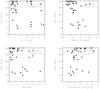	Fig. 3 Same as Fig. 2 but for the FSU-A lock ratio.
In the text

	Fig. 4 Upper panel: N band dispersion measured by EWS on MIDI data (red points) and predicted values using the K band data from FSU-A (blue points). Middle panel: measured (blue) and predicted (red) N band group delay values. Lower panel: group delay residual between measurement and prediction.
In the text

Fig. 5 Raw correlated flux of star HD 56470 (IRAS flux density FN = 0.47 Jy Beichman et al. 1988) observed during a PRIMA commissioning run (December 12, 2009) using the ATs with the MIDI+FSU-A mode. The light blue vertical lines are the formal errors as produced by EWS. The strong ozone absorption feature between 9.3 μm and 10.0 μm is clearly visible in the plot and marked by the vertical gray region. For wavelengths beyond ~11.7 μm, the source flux of faint N band targets drops to lower atmospheric transmission and cannot be measured at high accuracy because of high thermal background.

In the text

	Fig. 6 Same as Fig. 5 but for the FN = 50 mJy source TYC 5282- 2210-1 using the UTs. The blue line is a stellar photospheric fit to WISE (Wright et al. 2010) photometry for an independent confirmation of the measured N band flux density.
In the text

	Fig. 7 Illustration of the individual reduction steps for a synthetic white light pixel. a) Raw fringe scan. b) Normalized fringe scan; i.e., flat field and sky background correction were applied. Superimposed in blue and green are the extracted photometries of telescope beam T1 and T2. c) Photometric calibrated and normalized interferogram. See text for explanation.
In the text

	Fig. 8 Contour plot of a wavelet transform of the white light pixel of a single scan. The redder the color, the higher the wavelet power. The contours are plotted on a logarithmic scale.
In the text

	Fig. 9 Measured μ2 values obtained from a scan of the used calibrator star HD 152161 for all pixels of “AC” (in blue) and “BD” (in gray).
In the text

Fig. 10 Upper plots: transfer functions T2 for “AC” and “BD” for each spectral pixel and calibrator observation. The values for the individual spectral pixels are color-coded with respect to their corresponding wavelength (see legend in the upper left). The dashed lines are the corresponding 95% confidence intervals of the polynomial fits shown as solid lines. They gray data points are the computed T2 values for the time of the science observation. Lower plots: calibrated visibilities for each spectral pixel.

In the text

	Fig. 11 Fit of a binary model (green line) to the individual FSU-A visibility measurements (black points) for all spectral pixel of “AC” and “BD” for HD 155826. The red line is the predicted visibility variation based on the published orbit by Mason et al. (2010).
In the text

Fig. 12 Astrometric orbit by Mason et al. (2010) of HD 155826. The published orbit (see Table 2) is shown as a red solid line, the dash dotted line is the line of nodes. The black points are individual measurements retrieved from the Washington Double Star Catalog. The green point is the new astrometric point based on FSU-A visibility measurements. The solid lines connecting the individual measurements with the orbit indicate the expected position for the given orbital solution.

In the text

	Fig. 13 Same as Fig. 12 but for 24 Psc.
In the text

References

- Beichman, C. A., Neugebauer, G., Habing, H. J., Clegg, P. E., & Chester, T. J. 1988, Infrared astronomical satellite (IRAS) catalogs and atlases, Vol. 1: Explanatory supplement, 1 [Google Scholar]
- Bevington, P. R., & Robinson, D. K. 2003, Data reduction and error analysis for the physical sciences (Boston: McGraw-Hill) [Google Scholar]
- Boley, P. A., Linz, H., van Boekel, R., et al. 2013, A&A, 558, A24 [NASA ADS] [CrossRef] [EDP Sciences] [Google Scholar]
- Burtscher, L., Meisenheimer, K., Tristram, K. R. W., et al. 2013, A&A, 558, A149 [NASA ADS] [CrossRef] [EDP Sciences] [Google Scholar]
- Colavita, M. M., Booth, A. J., Garcia-Gathright, J. I., et al. 2010a, PASP, 122, 795 [NASA ADS] [CrossRef] [Google Scholar]
- Colavita, M. M., Serabyn, E., Ragland, S., Millan-Gabet, R., & Akeson, R. L. 2010b, in SPIE Conf. Ser., 7734, 23 [Google Scholar]
- Delplancke, F. 2008, New Astron. Rev., 52, 199 [NASA ADS] [CrossRef] [Google Scholar]
- Gitton, P. B., Leveque, S. A., Avila, G., & Phan Duc, T. 2004, in SPIE Conf. Ser., ed. W. A. Traub, 5491, 944 [Google Scholar]
- Haguenauer, P., Abuter, R., Andolfato, L., et al. 2012, in SPIE Conf. Ser., 8445 [Google Scholar]
- Jaffe, W., Meisenheimer, K., Röttgering, H. J. A., et al. 2004, Nature, 429, 47 [NASA ADS] [CrossRef] [PubMed] [Google Scholar]
- Jaffe, W. J. 2004, in New Frontiers in Stellar Interferometry, ed. W. A. Traub, SPIE Conf. Ser., 5491, 715 [Google Scholar]
- Kervella, P., Ségransan, D., & Coudé du Foresto, V. 2004, A&A, 425, 1161 [NASA ADS] [CrossRef] [EDP Sciences] [Google Scholar]
- Koresko, C., Colavita, M. M., Serabyn, E., Booth, A., & Garcia, J. 2006, in SPIE Conf. Ser. 6268 [Google Scholar]
- Le Bouquin, J.-B., Abuter, R., Bauvir, B., et al. 2008, in SPIE Conf. Ser., 7013, 33 [Google Scholar]
- Le Bouquin, J.-B., Berger, J.-P., Lazareff, B., et al. 2011, A&A, 535, A67 [NASA ADS] [CrossRef] [EDP Sciences] [Google Scholar]
- Leinert, C., Graser, U., Przygodda, F., et al. 2003, Ap&SS, 286, 73 [NASA ADS] [CrossRef] [Google Scholar]
- Lopez, B., Wolf, S., Lagarde, S., et al. 2006, in SPIE Conf. Ser., 6268 [Google Scholar]
- Mason, B. D., Hartkopf, W. I., & Tokovinin, A. 2010, AJ, 140, 735 [NASA ADS] [CrossRef] [Google Scholar]
- Mérand, A., Coudé du Foresto, V., Kellerer, A., et al. 2006, in SPIE Conf. Ser., 6268, 46 [Google Scholar]
- Müller, A., Pott, J.-U., Morel, S., et al. 2010, in SPIE Conf. Ser., 7734, 60 [Google Scholar]
- Nijenhuis, J., Visser, H., de Man, H., et al. 2008, in SPIE Conf. Ser., 7013 [Google Scholar]
- Olofsson, J., Henning, T., Nielbock, M., et al. 2013, A&A, 551, A134 [NASA ADS] [CrossRef] [EDP Sciences] [Google Scholar]
- Pepe, F., Queloz, D., Henning, T., et al. 2008, in SPIE Conf. Ser., 7013, 105 [Google Scholar]
- Peron, M., & Grosbol, P. 1997, in Optical Telescopes of Today and Tomorrow, ed. A. L. Ardeberg, SPIE Conf. Ser., 2871, 762 [Google Scholar]
- Petrov, R. G., Malbet, F., Weigelt, G., et al. 2007, A&A, 464, 1 [NASA ADS] [CrossRef] [EDP Sciences] [Google Scholar]
- Pott, J.-U., Müller, A., Karovicova, I., & Delplancke, F. 2012, in SPIE Conf. Ser., 8445 [Google Scholar]
- Ratzka, T., Schegerer, A. A., Leinert, C., et al. 2009, A&A, 502, 623 [NASA ADS] [CrossRef] [EDP Sciences] [Google Scholar]
- Sahlmann, J., Ménardi, S., Abuter, R., et al. 2009, A&A, 507, 1739 [NASA ADS] [CrossRef] [EDP Sciences] [Google Scholar]
- Sahlmann, J., Abuter, R., Ménardi, S., et al. 2010, in SPIE Conf. Ser., 7734, 62 [Google Scholar]
- Sarazin, M., & Tokovinin, A. 2002, in European Southern Observatory Conf. Workshop Proc., eds. E. Vernet, R. Ragazzoni, S. Esposito, & N. Hubin, 58, 321 [Google Scholar]
- Schmid, C., Abuter, R., Merand, A., et al. 2012, in SPIE Conf. Ser., 8445 [Google Scholar]
- Schuhler, N. 2007, Ph.D. Thesis, Université de Strasbourg [Google Scholar]
- Shao, M., & Staelin, D. H. 1977, J. Opt. Soc. Am., 67, 81 [Google Scholar]
- van Belle, G. T., Sahlmann, J., Abuter, R., et al. 2008, The Messenger, 134, 6 [NASA ADS] [Google Scholar]
- van Boekel, R., Min, M., Leinert, C., et al. 2004, Nature, 432, 479 [NASA ADS] [CrossRef] [PubMed] [Google Scholar]
- Wright, E. L., Eisenhardt, P. R. M., Mainzer, A. K., et al. 2010, AJ, 140, 1868 [NASA ADS] [CrossRef] [Google Scholar]
All Tables
Orbital elements (period P, semimajor axis a, inclination i, longitude of the ascending node Ω, epoch of periastron passage T0, eccentricity e, longitude of periastron ω) of HD 155826 and 24 Psc as published by Mason et al. (2010).