| Issue |
A&A
Volume 566, June 2014
|
|
|---|---|---|
| Article Number | A86 | |
| Number of page(s) | 14 | |
| Section | Galactic structure, stellar clusters and populations | |
| DOI | https://doi.org/10.1051/0004-6361/201323052 | |
| Published online | 19 June 2014 | |
Monte Carlo simulations of post-common-envelope white dwarf + main sequence binaries: comparison with the SDSS DR7 observed sample
1 Departament de Física Aplicada, Universitat Politècnica de Catalunya, c/Esteve Terrades 5, 08860 Castelldefels, Spain
e-mail: This email address is being protected from spambots. You need JavaScript enabled to view it.
2 Institute for Space Studies of Catalonia, c/Gran Capità 2–4, Edif. Nexus 104, 08034 Barcelona, Spain
3 Departamento de Física y Astronomía, Universidad de Vaparaíso, Avda. Gran Bretaña 1111, Casilla 5030, Valparaíso, Chile
4 Kavli Institute for Astronomy and Astrophysics, Peking University, 100871 Beijing, PR China
5 Observatoire Astronomique de Strasbourg, Université de Strasbourg, CNRS, UMR 7550, 11 rue de l’Université, 67000 Strasbourg, France
6 Department of Physics, University of Warwick, Coventry CV4 7AL, UK
Received: 14 November 2013
Accepted: 17 April 2014
Abstract
Context. Detached white dwarf + main sequence (WD+MS) systems represent the simplest population of post-common envelope binaries (PCEBs). Since the ensemble properties of this population carries important information about the characteristics of the common-envelope (CE) phase, it deserves close scrutiny. However, most population synthesis studies do not fully consider the effects of the observational selection biases of the samples used to compare with the theoretical simulations.
Aims. Here we present the results of a set of detailed Monte Carlo simulations of the population of WD+MS binaries in the Sloan Digital Sky Survey (SDSS) Data Release 7.
Methods. We used up-to-date stellar evolutionary models, a complete treatment of the Roche lobe overflow episode, and a full implementation of the orbital evolution of the binary systems. Moreover, in our treatment we took the selection criteria and all the known observational biases into account.
Results. Our population synthesis study allowed us to make a meaningful comparison with the available observational data. In particular, we examined the CE efficiency, the possible contribution of internal energy, and the initial mass ratio distribution (IMRD) of the binary systems. We find that our simulations correctly reproduce the properties of the observed distribution of WD+MS PCEBs. In particular, we find that once the observational biases are carefully considered, the distribution of orbital periods and of masses of the WD and MS stars can be correctly reproduced for several choices of the free parameters and different IMRDs, although models in which a moderate fraction (≤10%) of the internal energy is used to eject the CE and in which a low value of CE efficiency is used (≤0.3) seem to fit the observational data better. We also find that systems with He-core WDs are over-represented in the observed sample, because of selection effects.
Conclusions. Although our study represents an important step forward in modeling the population of WD+MS PCEBs, the still scarce observational data preclude deriving a precise value of the several free parameters used to compute the CE phase without ambiguity or ascertaining which the correct IMRD might be.
Key words: white dwarfs / binaries: general / stars: statistics / Galaxy: stellar content
© ESO, 2014
1. Introduction
Close-compact binaries are at the heart of several interesting phenomena in our Galaxy and in other galaxies. In particular, cataclysmic variables, low-mass X-ray binaries, or double degenerate white dwarf (WD) binaries – just to mention the most important and well studied ones – are systems that not only deserve attention by themselves, but also their statistical distributions are crucial to understanding the underlying physics of the evolution during a common envelope episode. Actually, the vast majority of close-compact binaries are formed through at least one CE episode. This phase occurs when the more massive star, hereafter the primary, fills its Roche lobe during the first giant branch or when it climbs the asymptotic giant branch (AGB). The mass transfer episode is dynamically unstable, and the envelope of the giant star engulfs the less massive star, i.e. the secondary, forming a common envelope (CE) around both the core of the primary (the future compact star) and the secondary star. Drag forces transfer orbital energy and angular momentum to the envelope, leading to a dramatic decrease in the orbital separation and to the ejection of the CE. If the system survives the CE phase, the outcome is a post-CE binary (PCEB) formed by a compact object and the main sequence (MS) companion with a much shorter orbital period separation than for the original main sequence binary system. The PCEBs studied in detail in this paper are those in which the compact object is a WD.
Even though the basic concepts of the evolution during a CE phase are rather simple, the details are still far from being well understood. This is so because several complex physical processes play an important role in the evolution during the CE phase. For instance, the spiral-in of the core of the primary and of the secondary and the ejection of the envelope are not only a consequence of the evolution of the core and remaining layers of the donor star in response to rapid mass loss, but also of tidal forces and viscous dissipation in the CE, which play key roles. Moreover, these physical processes occur on very different timescales and on a wide range of physical scales – see Taam & Ricker (2010) for a recent review. Consequently, any self-consistent modeling of the CE phase requires detailed hydrodynamical models that are not available at the present time, although recent progress is encouraging – see Ricker & Taam (2012, and references therein). The CE phase has therefore been traditionally described using parametrized models.
There are two canonical formalisms to treat the evolution during a CE episode. The most commonly used one, known as the α formalism, assumes energy conservation (Webbink 1984; de Kool 1990; Dewi & Tauris 2000). The second formalism is based on angular momentum conservation and is known as the γ formalism (Nelemans & Tout 2005). Within the α formalism, the energy transferred to the envelope is parametrized using an efficiency parameter, αCE. Furthermore, the binding energy of the envelope is also modeled with another free parameter, λ, which mainly depends on the mass of the donor and on its evolutionary stage. The most recent formulations also include a third parameter, αint, which is used to measure the fraction of the internal energy contributing to the ejection of the envelope. We postpone a precise definition of these parameters to Sect. 2.2, but we emphasize here that these parameters are still poorly determined. Thus, studying the population of binaries that have undergone a CE episode is important because some of their characteristics, such as the distribution of orbital periods and primary and secondary masses, can be used to constrain their values.
Binary systems formed by a WD and a MS companion are intrinsically one of the most common, and structurally simplest, populations of PCEBs. Thus, the statistical properties of this population are expected to provide crucial observational input that is needed to improve the theory of CE evolution (Davis et al. 2010; Zorotovic et al. 2010; De Marco et al. 2011; Rebassa-Mansergas et al. 2012). However, until now, detailed population synthesis studies have failed to effectively constrain the free parameters involved in the formulation of the CE phase, owing to an utter lack of observational data; see, e.g., de Kool (1992); Willems & Kolb (2004); Politano & Weiler (2007); and Davis et al. (2010). In particular, it has been shown that the early sample of well studied PCEBs is not only small but, because it is drawn mainly from “blue” quasar surveys, it is also heavily biased toward young systems with low-mass secondary stars (Schreiber & Gänsicke 2003). However, the SDSS (Frieman et al. 2008; Abazajian et al. 2009) has allowed a large number of WD+MS binaries to be identified (Heller et al. 2009; Rebassa-Mansergas et al. 2013), and a dedicated radial velocity survey of them has provided the so far largest and most homogeneous sample of close-compact binaries with available orbital periods (Rebassa-Mansergas et al. 2008; Nebot Gómez-Morán et al. 2011)
Recently, Toonen & Nelemans (2013) have presented binary population models of WD+MS PCEBs taking some of the observational selection effects important for the SDSS sample into account. However, while representing an important step forward, the conclusions that can be drawn from their study are limited by their assumption of a constant value for the binding energy parameter and by not taking into account possible contributions from the internal energy stored in the envelope. In this paper we describe the results of a detailed population synthesis study of WD+MS PCEBs in the Galaxy, modeling all the observational selection effects that affect the observed population in the well-characterized sample of PCEBs detected in the SDSS Data Release (DR) 7. A direct comparison of the simulated and the observed samples of PCEBs is performed as well, with the ultimate aim of constraining the current theories of CE evolution.
The paper is organized as follows. Section 2 describes the main ingredients of our Monte Carlo simulator, whereas in Sect. 3 the filters applied in order to take the observational biases into account are discussed in depth. The observed sample to which the simulations will be compared is presented in Sect. 4, while Sect. 5 presents the main results of our simulations, followed by an exhaustive analysis of the role played by some of the parameters involved in the CE phase. Finally, Sect. 6 closes the paper with a summary of our main findings and our concluding remarks.
2. The simulated population of WD+MS PCEBs
We expanded an existing Monte Carlo code (García-Berro et al. 1999, 2004) specifically designed to study the Galactic population of single WDs to deal with the population of binaries in which one of the components is a WD. In this section we describe the most important ingredients of our Monte Carlo simulator in detail.
2.1. The Monte Carlo simulator
The basic ingredient of any Monte Carlo code is a generator of random variables distributed according to a given probability density. The simulations described in this paper were done using a random number generator algorithm (James 1990) that provides a uniform probability density within the interval (0, 1) and ensures a repetition period of ≳1018, which is virtually infinite for practical simulations. When Gaussian probability functions were needed, we used the Box-Muller algorithm as described in Press et al. (1986).
We randomly chose two numbers for the galactocentric polar coordinates (r,θ) of each synthetic star of the entire stellar population within approximately 5 kpc from the Sun and following the SDSS DR7 spectroscopic plate directions (Abazajian et al. 2009). The adopted density distribution followed an exponential law with a radial scale length of 3.5 kpc. The z coordinate was randomly chosen following an exponential law with scale height H = 250 pc. We assumed a percentage of binaries of 50%, and we normalized our simulated systems to the local disk mass density (Holmberg & Flynn 2000). Next we drew two more pseudo-random numbers: the first one for the mass on the MS, M1, of each simulated primary star – according to the initial mass function of Kroupa et al. (1993) – and the second for the time when each star was born – assuming a constant star formation rate. The adopted age of the Galactic disk was 10 Gyr. Since the initial mass ratio distribution (IMRD) is still a controversial issue, we used three different prescriptions for it. The first one consisted in a flat distribution n(q) = 1, with q = M2/M1 the mass ratio, where M1 and M2 are the masses of the primary and secondary stars, respectively. We also considered a distribution of secondary masses that depends inversely on the mass ratio, n(q) ∝ q-1, and a distribution proportional to the mass ratio, n(q) ∝ q. In all cases, we only took stars with masses ranging from 0.1 M⊙ to 30 M⊙ into account. In addition, orbital separations were randomly drawn according to a logarithmic probability distribution (Nelemans et al. 2001), f(a) ∝ lna for 3 ≤ a/R⊙ ≤ 106. Finally, the eccentricities were randomly chosen according to a thermal distribution (Heggie 1975), g(e) = 2e for 0.0 ≤ e ≤ 0.9.
Once the masses of the stars were known and the properties of the binary system assigned according to the previously explained procedures, each of the components was evolved. We did that using the analytical fits to detailed stellar evolutionary tracks of Hurley et al. (2000), which provide full coverage of the entire range of masses of interest from the zero-age main sequence (ZAMS) until advanced stages of evolution. These evolutionary fits provide all the relevant information such as radii, masses, luminosities, evolutionary timescales, but not the photometric properties (see Sect. 2.3). We note that the evolutionary sequences of Hurley et al. (2000) are conservative. Accordingly, to obtain realistic simulations mass loss must be included. We assumed that the evolution during the MS phase was conservative, and only after hydrogen starts burning in a shell did we consider mass losses. The adopted mass-loss rate was that of Reimers & Kudritzki (1978), for which we assumed an efficiency η = 0.5. The prescription of Vassiliadis & Wood (1993) was used in the AGB phase. In the case of moderately close binary systems, we also considered a tidally enhanced mass-loss rate (Tout & Eggleton 1988): ![Mathematical equation: \begin{eqnarray} \dot M =\dot M_{\rm R} \left[1+B_{\rm W} \max\left( \frac{1}{2}, \frac{R}{R_{\rm L}}\right)^{6}\right] \label{tidal} \end{eqnarray}](/articles/aa/full_html/2014/06/aa23052-13/aa23052-13-eq25.png) (1)where M and R are the mass and star radius, RL is the Roche-lobe radius, ṀR the standard Reimers’ mass-loss rate, and BW the enhanced mass-loss parameter. As shown below, we analyzed several models in which BW varies from 0 to 104. Angular momentum losses due to magnetic braking and gravitational radiation were taken into account, assuming disrupted magnetic braking (Schreiber et al. 2010). Also, tidal evolution, circularization, and synchronization were considered.
(1)where M and R are the mass and star radius, RL is the Roche-lobe radius, ṀR the standard Reimers’ mass-loss rate, and BW the enhanced mass-loss parameter. As shown below, we analyzed several models in which BW varies from 0 to 104. Angular momentum losses due to magnetic braking and gravitational radiation were taken into account, assuming disrupted magnetic braking (Schreiber et al. 2010). Also, tidal evolution, circularization, and synchronization were considered.
For those binary systems in which the primary component had enough time to evolve to the WD stage, three situations can be found. For detached systems in which no mass transfer episodes occur whatsoever, we adopted the initial-to-final mass relationship of Catalán et al. (2008) to obtain the mass of the WD. When the mass transfer was stable we employed the procedure detailed in Hurley et al. (2002), while if the mass transfer was unstable, i.e. if the system underwent a CE phase, we followed the procedure detailed in Sect. 2.2.
In all the three cases described previously the corresponding evolutionary properties of the resulting WD must be interpolated in the appropriate cooling tracks. For low-mass helium-core WDs (He WDs, MWD ≲ 0.5 M⊙), we adopted the evolutionary tracks of Serenelli et al. (2001). For intermediate-mass carbon-oxygen core WDs (C/O WDs, 0.5 ≲ MWD/M⊙ ≲ 1.1), we used the very recent cooling tracks of Renedo et al. (2010), which include the most up-to-date physical inputs. Finally, for the high-mass end (MWD ≳ 1.1 M⊙) of the WD mass distribution, composed of oxygen-neon core WDs (O/Ne WDs), we adopted the cooling sequences of Althaus et al. (2007) and Althaus et al. (2005). All these cooling tracks correspond to WDs with pure hydrogen atmospheres.
2.2. Evolution during the CE phase
The evolution during the CE phase was computed following the treatment of Hurley et al. (2002). In particular, the Roche-lobe radius is calculated according to the prescription of Eggleton (1983), and during the overflow episodes both rejuvenation and aging were taken into account. The final separation of a WD+MS pair after the CE phase was obtained using the usual prescription, ![Mathematical equation: \begin{eqnarray} \frac{a_{\rm f}}{a_{\rm i}}=\left( \frac{m_{\rm WD}}{M_{1}}\right) \left[1+\left( \frac{2}{\lambda\alpha_{\rm CE}r_{\rm L1}}\right) \left( \frac{M_{\rm env}}{M_{2}}\right)\right] ^{-1}, \label{CE} \end{eqnarray}](/articles/aa/full_html/2014/06/aa23052-13/aa23052-13-eq35.png) (2)where ai and af are the initial and final orbital separations, Menv is the mass of the envelope of the primary star at the beginning of the CE phase, and rL1 = RL1/ai, where RL1 is the radius of the primary at the onset of mass transfer, αCE is the CE efficiency and λ is the binding energy parameter. These two parameters are described in detail below.
(2)where ai and af are the initial and final orbital separations, Menv is the mass of the envelope of the primary star at the beginning of the CE phase, and rL1 = RL1/ai, where RL1 is the radius of the primary at the onset of mass transfer, αCE is the CE efficiency and λ is the binding energy parameter. These two parameters are described in detail below.
The CE efficiency parameter, αCE, describes the efficiency of ejecting the envelope, namely, of converting orbital energy into kinetic energy to eject the envelope. We then have  (3)where Ebind is the binding energy of the envelope of the primary, usually approximated by the gravitational energy, i.e.,
  (4)This is generally rewritten in a more compact and suitable way as
  (5)where λ is the binding energy parameter, which represents the ratio between the approximate and the exact expression of the binding energy. In passing, we note that this approximation is equivalent to assuming that the resulting WD is a point mass and that the envelope is a shell of homogeneous density located at distance λR1 from the core of the primary.
We recall here that Han et al. (1995) introduced a parameter αth to characterize the fraction of the internal energy that is used to expel the CE. As in Zorotovic et al. (2010), we use here the notation αint for this parameter to emphasize that it includes not only the thermal energy but also the radiation and recombination energy. According to this, Eq. (4) becomes  (6)One can include the effects of the internal energy in the binding energy parameter λ by equating Eqs. (5) and (6). Thus, λ clearly depends on the mass of the donor, its evolutive stage, and the fraction of the internal energy, αint, available for ejecting the envelope. Except for models in which a fixed value of λ was assumed, the values of λ were computed using a subroutine from the binary-star evolution (BSE) code of Hurley et al. (2002).
With these prescriptions we were able to produce a synthetic population of WD+MS binaries. For the rest of this paper, we focus on those systems that experienced a CE phase (PCEBs) and that are still detached.
2.3. Photometry
The Monte Carlo simulator described so far does not provide photometric magnitudes for the simulated WD+MS PCEBs. In this section we explain how we obtain ugriz SDSS magnitudes for the two binary components in an independent manner, which are then combined to obtain the magnitudes of the simulated sample of WD+MS PCEBs.
WD Johnson-Cousins UBVRI magnitudes were obtained from the evolutionary tracks detailed in the previous section (Serenelli et al. 2001; Renedo et al. 2010; Althaus et al. 2007). To transform to the SDSS ugriz system we simply followed the procedure explained in Jordi et al. (2006). The photometry of the companion stars was obtained as follows. We first used the empirical spectral type-mass relation of Rebassa-Mansergas et al. (2007) and obtained the spectral type of the secondary stars (the secondary star mass is known from the Monte Carlo simulator). This relation is only defined for M dwarfs (M ≲ 0.45 M⊙), however, as shown later (in Sect. 3.3), WD+MS pairs containing earlier type secondary stars are excluded from the simulated sample as a consequence of selection effects on the observed population of PCEBs.
For each spectral type we then obtained average u − g, g − r, r − i, and i − z colors by fitting a large sample of SDSS M dwarfs (West et al. 2008) to the M-dwarf templates of Rebassa-Mansergas et al. (2007). Once ∼25 to 30 stars were fitted for each spectral type, we then calculated the colors using the available SDSS dereddened magnitudes of the considered M dwarfs and averaged them. Our average colors are in very good agreement with those of West et al. (2011) for g − r, r − i, and i − z. For u − g this exercise works relatively well for spectral types M0−5, but it becomes rather uncertain for later spectral types. To avoid this we searched for nearby late-type M dwarfs (>M5) in the sample of Bochanski et al. (2011) with available dereddened magnitudes in SDSS and averaged their u − g colors. This dramatically reduced the uncertainties. Once the average colors were obtained, we used the empirical Mr − (r − i) and Mr − (i − z) relations of Bochanski (2008) to obtain Mr. This gives r with the known distance from the Monte Carlo simulator. The remaining ugiz magnitudes were easily calculated from the average colors. We emphasize that our procedure rests on a purely empirical basis, thus avoiding undesired biases due to using synthetic spectra, which mostly depend on the surface gravity and effective temperature, instead of M-dwarf template spectra, which essentially depend on the spectral type.
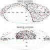 |
Fig. 1 Position of Legacy (black) and SEGUE (red) SDSS DR 7 WD+MS binaries in Galactic and equatorial coordinates. Taken from Rebassa-Mansergas et al. (2012). (Color version online.) |
Once the SDSS ugriz magnitudes of the two binary components had been obtained, we added the corresponding fluxes to obtain the magnitudes of the simulated WD+MS PCEBs. Finally, in order to provide reliable magnitudes and colors (see Sect. 3.1) Galactic extinction was incorporated using the model of Hakkila et al. (1997), while the color correction was that of Schlegel et al. (1998).
3. Selection effects
So far we have described how we simulated the WD+MS PCEB population in the Galaxy in the directions of the SDSS DR7 spectroscopic plates and how we computed the SDSS ugriz magnitudes of the entire simulated sample. Given that the main purpose of this paper is to perform a detailed comparison of the simulated and the observed WD+MS binary populations in the SDSS that underwent a CE phase, it becomes necessary to incorporate the observational selection effects in a very realistic and detailed way. In this section we describe how we modeled these selection biases.
3.1. Color cuts
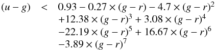
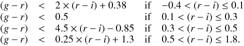
Our first step consisted in applying a color filter. The color cuts allow WD+MS binary systems to observationally culled from the spectroscopic SDSS DR7 WD+MS binary catalog (Rebassa-Mansergas et al. 2012). From this sample, we only considered systems observed by the SDSS Legacy survey (see Fig. 1), since WD+MS binaries identified by SEGUE – Sloan Extension for Galactic Understanding and Exploration (Yanny et al. 2009) – were selected following a completely different algorithm (Rebassa-Mansergas et al. 2012). For magnitudes within the range 15 <i< 19.5, the color cuts we applied to the synthetic sample were the following (see also Rebassa-Mansergas et al. 2013):
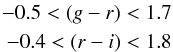 and
and
3.2. Spectroscopic completeness
The main science driver of the SDSS Legacy survey was to acquire spectroscopy for magnitude-limited samples of galaxies (Strauss et al. 2002) and quasars (Richards et al. 2002). Because of their composite nature, WD+MS binaries form a “bridge” in the color space that connects the WD locus with that of low-mass stars (Smolčić et al. 2004). The blue end of the bridge, characterized by WD+MS binaries with hot WDs and/or late type companions, strongly overlaps with the color locus of quasars, and was therefore intensively targeted for spectroscopy by the SDSS Legacy Survey. In contrast, the red end of the bridge is dominated by WD+MS binaries containing cool WDs and excluded from the quasar program. Thus, the next step in producing realistic simulations of the PCEB population is to apply a spectroscopic completeness correction that accounts for the probability of a given simulated PCEB with appropriate colors to be spectroscopically observed by the SDSS Legacy survey.
To estimate this probability we proceeded as follows. We first calculated the spectroscopic completeness of each WD+MS binary observed by the SDSS DR 7 Legacy Survey. It is important to keep in mind that these observed WD+MS binaries include wide systems that never interacted during their evolution and PCEBs and that only PCEBs are considered in the numerical sample. Strictly speaking we then should consider only those observed WD+MS binaries that are PCEBs. However, the number of identified PCEBs is just ∼10% of the entire SDSS WD+MS binary catalog (Rebassa-Mansergas et al. 2013), and we know that about one third of the total number of WD+MS binaries should be a PCEB (Schreiber et al. 2010). Besides, there is no reason to believe that the spectroscopic completeness will vary from wide to close WD+MS binaries. To avoid low number statistics in our calculations, we thus decided to use the entire observed sample, i.e. wide WD+MS plus PCEBs. We did, however, exclude WD+MS binaries that are resolved in their SDSS images, because they are associated with large uncertainties in their photometric magnitudes. The resulting sample contains 1645 systems.
We obtained the u − g, g − r, r − i, and i − z colors of each of our 1645 observed WD+MS binaries and defined a four-dimensional (one dimension per color) sphere of 0.2 color radius around each of them. Within each sphere we calculated, via DR 7 casjobs (Li & Thakar 2008) the number of point sources with clean photometry (Nphot), as well as the number of spectroscopic sources (Nspec). This search was restricted to those systems fulfilling the color cuts given in Sect. 3.1. The choice of a sphere radius of 0.2 ensures that Nspec is larger than 15 in each case. The spectroscopic completeness of each of the observed WD+MS systems is simply given by Nspec/Nphot. The probability that a simulated PCEB is observed spectroscopically by the Legacy survey of SDSS finally corresponds to the spectroscopic completeness of the observed WD+MS binary with the most similar colors, i.e., the closest color distance (as defined by the four colors) between the simulated WD+MS binary and the observed systems. After applying the color selection filter, the synthetic binaries occupy color regions densely populated by the observed WD+MS binaries. We find that, on average, the four-dimensional color distance from one synthetic WD+MS to the nearest observed target is 0.09, a fairly reasonable value, although this distance can in some cases be as small as 0.01, whereas only in ∼4% of the cases is it larger than 0.2.
3.3. Intrinsic WD+MS binary bias
It is expected that a given fraction of the simulated WD+MS PCEBs should contain primary or secondary stars that would be undetectable in the spectrum if observed spectroscopically by the SDSS. This is the case when one of the stellar components is considerably brighter than the other and outshines the companion. For late-type secondary stars, this implies an upper limit on the WD effective temperature, at which we would be able to discern the companion in the SDSS spectrum. Conversely, the detection of WDs next to early-type companions results in a lower limit on the WD effective temperature. In addition, SDSS spectra of farther objects are associated with a lower signal-to-noise ratio. Our observed sample of WD+MS PCEBs is partially based on the visual identification of both binary components in the SDSS spectrum (Rebassa-Mansergas et al. 2010), and consequently objects with low signal-to-noise ratio may not have passed the identification criteria. This implies an upper limit in the distance of WD+MS binaries. These two effects need to be considered in our simulated sample of WD+MS PCEBs.
In order to evaluate these selection effects, we followed the approach adopted by Rebassa-Mansergas et al. (2011) and used the WD atmosphere models of Koester et al. (2005) and the M-dwarf templates of Rebassa-Mansergas et al. (2007) to obtain synthetic composite WD+MS binary spectra in the wavelength range and resolution provided by typical SDSS spectra for a wide range of WD effective temperatures (Teff ranging from 6000 to 100 000 K in 37 steps nearly equidistant in log Teff) and surface gravities (covering from log g = 6.5 to 9.5 in steps of 0.5), spectral type of the companions (M0−9, in steps of one subclass), and distances (from 50 to 1700 pc in steps of 50 pc). To the complete set of synthetic composite spectra, we added artificial Gaussian noise varying according to the distance used. Specifically, the noise level introduced to the composite spectra reproduces the signal-to-noise ratio that the observed WD+MS binary spectra have at the considered distance.
Once the synthetic spectra were obtained, we subjected the complete sample to the identification criteria defined for real WD+MS binary spectra in SDSS, namely a visual inspection of the spectra and a search for blue and red excess in those spectra dominated by the flux of the secondary star and WD components, respectively (see Rebassa-Mansergas et al. 2010, for details). In addition we calculated the ugriz magnitudes from the synthetic spectra and excluded all systems exceeding the magnitude limits given in Sect. 3.1. From the resulting sample we then evaluated the WD effective temperature and distance limits that were then applied according to the sample of WD+MS binaries obtained from the Monte Carlo simulator.
3.4. PCEB orbital period filter
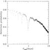 |
Fig. 2 Detection probability of a PCEB as a function of the orbital period. |
Finally, we filtered our simulated binary systems according to a period efficiency function, which measures the probability of identifying a PCEB among the WD+MS SDSS sample. The detection probability function (Nebot Gómez-Morán et al. 2011) is shown in Fig. 2. As can be seen, the probability of finding a binary system decreases for increasing periods, and drops rapidly for those systems with period longer than three days. For orbital periods of one day or multiples of one day the probability for sampling the same orbital phase increases, which translates into a decrease in the period efficiency function.
4. The observed sample
The sample of binary systems that we use for comparison consisted on 53 WD+MS PCEBs from the SDSS DR7 catalogue with known periods (see Rebassa-Mansergas et al. 2012; Nebot Gómez-Morán et al. 2011; Zorotovic et al. 2010, and references therein). As we already mentioned, SEGUE systems have been excluded. The periods are well determined, and therefore the distribution of periods is useful for comparing with the period distribution obtained for the simulated systems. To compare with our models, we are also interested in knowing the core composition of the WD in the observed systems, so as to estimate the fraction of systems containing He WDs, and also the number of systems containing more massive O/Ne WDs. To do this we proceeded as follows. If the mass of a WD is lower than 0.5 M⊙ we assumed that it has a He core. Conversely, if the mass of a WD is greater than 0.5 M⊙ but lower than 1.1 M⊙ a C/O core was adopted. Finally, if the mass of the WD is higher than 1.1 M⊙, an O/Ne core was adopted. For 49 of the 53 PCEBs in the sample, it has been possible to determine the mass of the WD using the method described by Rebassa-Mansergas et al. (2007). As in Zorotovic et al. (2010), to determine their compositions, we decided to exclude systems with WD temperatures below 12 000 K, because the spectral fitting methods are not reliable for cooler WDs and therefore their masses can not be trusted. This implies that reliable WD masses can be obtained for 40 of the 53 systems that form our observed sample, of which 14 have a He WD, 23 a C/O WD, and 2 an O/Ne WDs. There is also one system with MWD = 0.5 M⊙ for which we cannot decide which type of WD it is. This corresponds to a fraction of 36 ± 8% of He WDs in the sample, where we have assumed binomial errors. This issue, nevertheless, is discussed in more detail in Sect. 5.5.
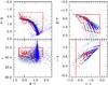 |
Fig. 3 Color–color diagram of the synthetic WD+MS PCEBs obtained using our Monte Carlo simulator when our reference model (αCE = 1.0, λ = 0.5, and n(q) = 1) is employed. Systems containing He WDs are represented using black dots, while blue dots correspond to systems with C/O or O/Ne WDs. The observed WD+MS PCEB systems are displayed using red dots. The color selection criteria are shown using red lines (Sect. 3.1). (Color version online.) |
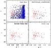 |
Fig. 4 Color–magnitude diagram of the synthetic WD+MS PCEBs obtained using our Monte Carlo simulator (blue and black dots) compared with the observed systems (red symbols) after applying the different filters explained in the text to our reference model. Colors are the same as in Fig. 3. (Color version online.) |
5. Results
We computed a large number (∼500) of Monte Carlo simulations covering a wide range of values of the CE efficiency parameter, 0.0 ≤ αCE ≤ 1.0, and the fraction of the internal energy available to eject the CE, 0.0 ≲ αint ≲ 0.3, which can result in very high values of the binding energy parameter, λ. We also performed simulations in which λ was computed including the contribution of different fractions of the internal energy, αint. All this was done for the three IMRDs, n(q), previously mentioned in Sect. 2.1. For each of our models we generated ten independent Monte Carlo simulations (with different initial seeds) and for each of these Monte Carlo realizations, we increased the number of simulated Monte Carlo realizations to 104 using bootstrap techniques. Specifically, we used the resampling method described in Chernick (2007) in all our calculations. The method consists in generating resamples with a probability equal to that of the original sample. Each resample, also called a “bootstrap sample” or “replication”, must have the same size (number of elements) as the original sample. This is why this method is named resampling with replacement. Because resampling can be done without adopting any particular assumption about the probability distribution of the population, this technique can be used not only to derive the sample distribution-free values of interest, but also for assessing the precision and variability of sample statistics. In this way we were able to streamline the Monte Carlo calculations, with large savings of computer time. Moreover, using this procedure we ensured convergence in all the final values of the relevant quantities. In what follows we describe the model predictions and compare them with the observations. Given that the parameter space of CE evolution is very large, we show in this paper only those results that imply some relevant differences between the corresponding models.
5.1. Color–color space
We first investigate whether the simulated PCEB population is placed in the same regions in the color–color space as the observed PCEBs. To that end and for the sake of definiteness, we define a reference model for which we considered αCE = 1.0, λ = 0.5, and a flat IMRD, n(q) = 1. This choice of parameters should not be considered as a representative case, and we use it just to illustrate the effects of the different filters applied to the simulated samples. Moreover, we adopted this model because it represents an extreme (albeit frequently employed) case among the many possible choices of the free parameters of common envelope evolution. Figure 3 shows an example of the color–color diagram of present-day WD+MS PCEBs obtained in a typical Monte Carlo realization for our reference model. We show systems that underwent the CE phase before He ignition (case B) a nd contain He WDs, systems that underwent the CE episode after He ignition during the early AGB (case C) or during the thermally pulsing AGB phase (TPAGB), and contain C/O or O/Ne WDs, as well as the sample of observed WD+MS PCEBs. The different color cuts discussed in the Sect. 3.1 are represented by red lines. A quick look at Fig. 3 reveals that our simulations recover the observed population of WD+MS PCEBs fairly well in the different color–color diagrams, and that our synthetic WD+MS PCEBs overlap with the real ones. Moreover, our simulated population lies within the region allowed by the different color cuts. However, as expected, the entire simulated Galactic population of PCEBs occupies a larger region than the observational one, especially in the i vs. g − r color–magnitude diagram. Finally, we note as well that the discrete blue tracks come our mapping MS stars onto discrete spectral types.
5.2. The effects of biases and selection criteria
Total number and percentage of simulated WD+MS binary systems obtained after applying the successive selection criteria.
The effect of each filter over the simulated WD+MS PCEBs is illustrated in Fig. 4 for our reference model in the g − r versus i color–magnitude diagram. Each panel represents the systems that survive after consecutively applying the filter indicated on it. We show the effect of the color selection filter (upper left panel), the result of applying the spectroscopic completeness filter (upper right panel) to the previous sample, the effect of using the intrinsic binary bias filter (lower left panel), and finally the result after using the period filter (lower right panel).
As can be seen, the different filters applied to the original synthetic sample (black and blue dots) severely reduce the total number of observable objects, which is consistent (within an order of magnitude) with the observed sample (red symbols). Moreover, the final sample for this specific Monte Carlo simulation shows poor agreement with the observed one. In particular, for this specific simulation the observed binaries occupy a region that is systematically bluer and brighter than that of the synthetic sample. The reason for this is twofold. The first is the otherwise natural intrinsic dispersion of any Monte Carlo simulation. Given the now few synthetic binaries surviving the different cuts, and the scarce observational data, these effects can become prominent in a particular Monte Carlo sample. However, the most important reason is that, as already mentioned, the set of theoretical parameters adopted for this specific model – namely the choice of αCE, λ, and n(q) – is clearly excluded by the observations, and we only adopted it for illustrative purposes, given that this is a set of parameters that is frequently employed in the literature. More elaborated models, which fit the observational data better, will be discussed below, in Sects. 5.6, and 5.7.
To quantitatively analyze the effects of the different selection criteria on the entire population of simulated WD+MS PCEBs, we show in Table 1 the total number and percentage (in parentheses) of WD+MS PCEBs initially simulated and obtained after applying consecutively the selection criteria and observational biases described in Sects. 3.1 to 3.4. We also list the cumulative percentage of the WD+MS population in the last column of this table obtained after applying the selection cuts. We show the results for three representative models. Model 1 is our reference model, previously described. In Model 2 we also used αCE = 1.0 and λ = 0.5, but we adopted n(q) ∝ q-1, to illustrate the effects of the IMRD. Finally, for Model 3 we adopted αCE = 0.3 and n(q) ∝ q-1, while λ was computed for every binary assuming αint = 0.2. The unfiltered samples, which correspond to the total number of WD+MS PCEBs in the SDSS DR7 fields irrespective of their apparent magnitude, are sufficiently large in all three cases and allow us to study the effects of the succesive filters.
The selection criteria produce a dramatic decrease in the total number of simulated WD+MS PCEBs, independently of the adopted model. In particular, the final simulated population is smaller than 0.1% of the initial sample for all three models – see the last column of this table. The most restrictive selection criteria are the color cuts and the spectroscopic completeness filter. Only ∼7% of the objects in the input sample pass the cuts in color and magnitude for all three models, while the spectroscopic completeness filter eliminates ∼97% of those that survive the first filter. If only these two filters are applied, the total population of potentially observable systems decreases drastically down to 0.2–0.3% of the unfiltered sample.
This behavior can be explained easily. First, the SDSS only covered 15 <i< 19.5 and most WD+MS binaries in our Galaxy are obviously fainter. Second, the SDSS was primarily designed to detect galaxies and quasars and thus the probability that a WD+MS binary system is spectroscopically detected by the SDSS is relatively small, specially for WD+MS binaries containing cool WDs (Rebassa-Mansergas et al. 2013). The remaining filters, i.e. the intrinsic binary bias filter and the period filter, reduce the size of the sample of simulated PCEBs systems further. In particular, the intrinsic binary bias filter reduces the number of systems surviving the spectroscopic completeness filter to about 30% to 40%, while the period filter reduces the sample of systems that survive the spectroscopic completeness filter to ∼60%. Thus, the selection criteria play a crucial role since only ∼0.05% of the simulated binary systems survive the successive filters.
The final number of WD+MS PCEBs predicted to be identified by the SDSS is in reasonable agreement with the observed number of systems (see Table 1). This indicates that both our initial assumptions and the computation of the selection effects and biases are likely to be good representations of reality. However, it is important to realize that the number of predicted PCEBs depends somewhat on the adopted values of αCE and λ during the CE phase. We obtain the best agreement (i.e., the largest number of predicted systems) by assuming a variable binding energy parameter and a low CE efficiency, namely for Model 3.
Interestingly, the selection criteria employed to select the sample introduce an unexpected bias into the observed population of WD+MS PCEBs, as the fraction of systems containing He WDs that are finally culled from the total population increases independently of the model, from ∼25–35% to ∼60–70%. This implies that the observed population of WD+MS PCEBs is severely biased as a consequence of the selection criteria employed to cull it and that WD+MS PCEBs containing a He WD are over-represented in the final sample, independently of the adopted model, owing to the observational selection effects.
5.3. The role of the enhanced mass-loss parameter
It has been suggested that the presence of a close companion could enhance mass loss during the red giant phase (Tout & Eggleton 1988). As shown in Eq. (1) the mass-loss tidal enhancement depends on a parameter, BW, that is unknown at present. To evaluate the influence of this parameter on the resulting population of WD+MS PCEBs and to better constrain the value of this enhancement parameter, we performed an additional set of simulations in which we adopted several values for BW, ranging from 0 (no tidal enhancement) to 103. The results of such simulations are presented in Table 2, where we show the percentages of He and C/O (or O/Ne) WDs in WD+MS PCEBs for several values of BW, after applying all the selection effects to the three models previously described in Sect. 5.2. These percentages are computed as the ensemble average of a sufficiently large number of individual Monte Carlo realizations, for which we also compute the corresponding standard deviations. Both are listed in Table 2.
Enhanced mass-loss parameter and percentage of PCEBs with different types of WDs.
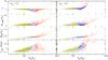 |
Fig. 5 From top to bottom: binding energy parameter, primary ZAMS mass, WD mass and orbital period as a function of the Roche-lobe radius of the primary, as given in Eggleton (1983). The case B, case C and TPAGB case CE episodes are represented using green, blue and red dots, respectively. The two sides show the results for two models in which αCE = 0.3 and n(q) = 1 but without and with a fraction of the internal energy contributing to expel the envelope: αint = 0.0 (left panels) and αint = 0.2 (right panels). (Color version online.) |
In general, the percentage of He WDs increases as log BW increases. The He WD fraction increases because as BW is increased the mass losses are greater. Increased mass loss leads to an increase of the orbital separation and increases the mass ratio q. This can cause the systems not to fill their Roche lobe, to end up with a longer orbital period, or to stable mass transfer instead of evolving through a CE episode. These effects are strongest for systems that without increased mass loss, would fill their Roche lobe on the AGB since these systems evolve through the entire sub-giant and first giant branch. Thus, increased mass loss leads to a reduced fraction of C/O and O/Ne white dwarfs in PCEBs, while the number of PCEBs that contain He-core WDs remains approximately constant. We stress that even for a low value of the enhancement parameter, the percentage of He WDs is somewhat high, at odds with the observational data set we are using to compare, for which the fraction of He WDs is ∼40% (see Sect. 4). Consequently, low values of BW seem to be more compatible with the observational data. For this reason, in the simulations described in what follows we adopted BW = 0, which is a conservative choice.
5.4. The effects of the internal energy
Percentage of systems with He WDs and KS test of the period distribution for six representative models with λ = 0.5.
For more than a decade, we know that assuming a constant binding energy parameter λ is probably not a good approximation (Dewi & Tauris 2000). Instead, λ depends on the mass of the donor star and the evolutionary stage. We explore this in Fig. 5 where we show from top to bottom: the distributions of the binding energy parameter (λ), primary ZAMS masses, WD masses, and periods, as a function of the radius of the primary just prior to the CE episode, i.e. of its Roche-lobe radius. We compare here two models, both with αCE = 0.3 – which is consistent with the results of Zorotovic et al. (2010) – and n(q) = 1, but with αint = 0.0, or αint = 0.2, respectively. We chose these two particular models to highlight the effects of including a fraction of the internal energy of the envelope that helps in the ejection process. The lefthand panels of Fig. 5 display the results for the model in which αint = 0.0, while the right-hand ones are for the model with αint = 0.2.
We show using different symbols systems that have experienced a case B CE episode, WD+MS systems that underwent a case C CE episode and those where a TPGAB CE episode took place. As can be seen in this figure for those models in which no internal energy is available to eject the envelope, the value of λ remains practically constant, and it has a relatively small dispersion that first increases with increasing Roche-lobe radius, until it reaches a maximum at RL ∼ 200 R⊙, and then decreases again for higher values of RL (see the top left panel of Fig. 5). On the other hand, when a moderate amount of internal energy is available to eject the envelope, we find an overall enhancement of the resulting values of λ (top right panel of Fig. 5). This was expected since the contribution of the internal energy becomes more important for more extended envelopes, where the gravitational energy becomes lower and the envelope is less tightly bound. Moreover, this enhancement is more noticeable for the highest values of the Roche-lobe radius at which the CE episode occurs.
We also find that the dispersion in the values of λ increases for wider systems. In this sense, we emphasize that the top left and right panels Fig. 5 actually show which binary systems have prominent contributions of the internal energy are prominent. The progenitors of systems with He-core WDs fill their Roche lobe on the first giant branch where only a very small amount of internal energy is stored in the envelope. Thus, for those systems, increasing the value of αint does not lead to an increased value of λ and has virtually no effect on the outcome of CE evolution. The distributions of primary ZAMS masses and WD masses as a function of the Roche-lobe radius is fairly similar for both models (second and third panel from top, respectively).
Finally, the distribution of orbital periods is also very similar in both cases, except for a population of long-period (≳10 days) PCEBs, descending from the initially more separated systems. This is only observed when a fraction of the internal energy of the envelope is taken into account. In summary, the only relevant differences between both models are the distribution of the values of λ and the existence of systems with very long final periods, while the rest of the distributions are very similar.
Percentage of systems with He WDs and KS test of the period distribution for our models with αCE ≤ 0.3 and λ properly computed for each system, where different fractions of internal energy are taken into account.
5.5. The fraction of PCEBs containing He-WDs
One important and relatively robust value that can be derived from the observed sample is the fraction of PCEBs containing He-core WDs. Therefore, here we compare the percentage of WDs with He cores in the final sample of our simulations with that of the observed sample, which is around 40%.
In Table 3 we display the percentage of He WDs, as well as the results of a Kolmogorov-Smirnov (KS) test resulting from a comparison between the observed and the theoretical period distributions (we describe and discuss the KS test in Sect. 5.6), for some of the Monte Carlo simulations in which a fixed value of λ = 0.5 was adopted, for the three IMRDs. We emphasize that only a selected handful of models is shown for the sake of conciseness in this table. However, the actual number of models analyzed is much larger. As can be seen, a common feature of the synthetic distributions is the resulting large number of He WDs. Specifically, the results displayed in Table 3, and those obtained from similar models not explicitly shown here, show that only the models for which a low value of αCE is adopted produce the required percentage of He WDs. In particular, in all the models in which αCE is larger than 0.3 the fraction of WDs with He cores is significantly larger than the observed value, 36 ± 8%. This is true for all three IMRDs. We think that all the He WDs found in our Monte Carlo simulations is not a weakness of the models, but a potentially interesting feature that deserves further study. However, we judge that this result should be taken with some caution, because the core composition of the synthetic WDs is set by its evolutionary history and depends on the adopted mass limit between He and C/O WDs. Also, the observed fraction of He WDs depends crucially on the error in the mass determinations of the WDs in the sample of PCEBs WD+MS binaries in the SDSS. This issue has been explored before by Rebassa-Mansergas et al. (2011) – see, for instance, their Table 4 – who found that as the uncertainty in the mass estimates is typically ∼0.05–0.1 M⊙, the theoretically predicted clear separation between He and C/O WDs at MWD = 0.5 M⊙ is smeared out. As a result, the real observed fraction of He WDs in PCEBs WD+MS systems is still subject to some uncertainty, and needs to be better determined, since it might be possible that some of the He WDs instead have C/O cores.
Table 4 shows the same results but for the case in which λ is computed for different values of αint. Again, we do this for several values of αCE, αint (with αint ≤ αCE), and for the three IMRDs. Based on our previous results, we only show here the results for our models with αCE ≤ 0.3. Once again, the fraction of WDs with He cores is sensitive to the adopted value of αCE, and also a bit to αint. In particular, as αCE is increased, the percentage of He WDs also increases, independently of the adopted IMRD.
5.6. The orbital period distribution
The parameter of PCEBs that can be most accurately measured is the orbital period. Thus, comparing the predicted and observed orbital period distribution is crucial. We performed KS tests to estimate the similitude of the theoretical and observational period distributions. We restricted ourselves to models with α ≤ 0.3 as otherwise the fraction of PCEBs containing He-core WDs drastically disagrees with the observations (see previous section). All models with αCE ≤ 0.3 reproduce the observed orbital period distribution reasonably well which is indicated by KS-values exceeding 0.2. This means that there are no significant indications that the simulated and the observed distributions are different. We obtained the highest KS-values (exceeding 0.6) for models with αCE = 0.3. In what follows we describe the results in some more detail for those models that best fit the period distribution.
For the sake of conciseness we only considered those models with a KS value greater than 0.6, with a percentage of WD+MS PCEBs with He-core WDs below 70% – see Rebassa-Mansergas et al. (2011) for a detailed discussion of the percentage of He WDs in WD+MS PCEBs in the SDSS, and a small fraction (<6%) of O/Ne WDs, in accordance with the observed sample. Additionally, we required that the selected theoretical models had statistical properties similar to those of the observed sample of WD+MS binaries. These included a similar average period, as well as maximum and minimum periods of the synthetic binaries, after applying the successive filters in agreement with observations, and an assessment of the morphology of the global distribution of periods.
Once these criteria are employed we are left with only four models. The first model has αint = 0.2 and n(q) ∝ q-1, the second one αint = 0 and n(q) = 1, the third one αint = 0 and n(q) ∝ q, and finally the fourth one αint = 0.1 and n(q) ∝ q. All the models correspond to a CE prescription in which λ is computed for each binary. Among these four best models, there is a degeneracy between the adopted prescription for the CE phase and the IMRD. This implies that on the basis of the present observational data, we cannot determine which is the IMRD.
In Fig. 6 we compare the distribution of periods of the present-day WD+MS PCEBs simulated sample with the observational one. We show the period distributions for the entire sample of WD+MS PCEBs (bottom panel of each figure) but also separately for systems containing He WDs (middle panels) and C/O or O/Ne WDs (top panels). From the 40 systems with WD mass determination and WD temperature higher than 12 000 K described in Sect. 4, we found that six of them, with WD masses close to 0.5 M⊙, can contain either a He WD or a C/O WD, given their WD mass error. Of the 34 remaining systems, 11 contain a He WD and 23 a C/O or O/Ne WD. These are the systems that were considered for the middle and top panels, respectively, while the bottom panels contain the 53 systems with available periods. In general, our Monte Carlo simulations agree closely with the observational period distribution for the entire population. However, the still large observational error bars and the almost negligible differences between the different theoretical models preclude drawing definite conclusions about which is the best one. This indicates that the selection criteria dominate the final observational distribution. Nevertheless, a detailed inspection of Fig. 6 reveals that those models with non-zero internal energy present slightly extended tails in the long-period end of the distribution. Even though these tails possibly could not be statistically significant, their mere existence provides a hint that these models do not appropriately describe the ensemble properties of the period distribution of WD+MS PCEBs. Consequently, this compels us to consider those models with a small amount of internal energy as more convenient.
Statistics for the best models.
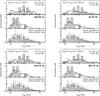 |
Fig. 6 Period histograms (normalized to unit area) of the distribution of present-day WD+MS PCEBs for our four best models (black line) compared with the observational distribution (dotted line, gray histogram). |
Table 5 contains the statistics obtained for our four best models. This table also shows that those models with non-zero values of the internal energy parameter have maximum periods that are much longer (a factor of ∼10) than the ones in which αint = 0.0 is adopted, while the minimum periods remain nearly the same. The average value for the periods is therefore larger when we include a fraction of internal energy, which is especially true for systems containing a C/O or an O/Ne WD. Those models in which no internal energy is available to eject the CE fit the measured average period of the observed distribution of WD+MS PCEBs (⟨ P ⟩ = 0.69 days) better. It is also interesting to remember that the internal energy becomes especially important for more evolved primaries, which have a more massive core (the future WD) and a more extended envelope. For this reason those simulations in which αint ≠ 0 have an enhanced production of WD+MS systems with an O/Ne WD, because it becomes easier for these systems to survive a CE phase thanks to this additional source of energy. This is an important fact, because in the observed sample there are only two WD+MS PCEBs in which the resulting WD has a mass higher than 1.1 M⊙. All in all, we conclude that to account for the ensemble properties of the distribution of periods and the detection of a small fraction of WD+MS PCEBs with very massive WDs, the fraction of the internal energy available to eject the envelope must be small.
It is also worth mentioning that the average periods for the two subpopulations of WDs with He and C/O or O/Ne cores, are markedly different, because that of WD+MS systems with He core WDs is significantly smaller than that of systems with more massive WDs. This agrees with the observational analysis of Zorotovic et al. (2011). If one separates He-core and C/O or O/Ne core systems, however, there are too few observed systems to separately compare model predictions and observations.
Finally, we note that although our population synthesis simulations reproduce the observed distribution of orbital periods with reasonable accuracy, this is not the case when the individual distributions for He WDs and C/O or O/Ne WDs are considered, a fact that is somewhat hidden by the normalization criteria employed in Fig. 6. This may be indicative of a missing piece of physics in the theoretical calculations or, as already mentioned, to a not entirely reliable determination of WD masses. However, the reader should keep in mind that the theoretical histograms presented in Fig. 6 are the result of averaging a large number of individual Monte Carlo realizations. In a typical Monte Carlo realization in which ∼15 WD+MS PCEBs are culled, the final distributions are more irregular and would be more similar to those observationally found. Clearly, additional studies are needed to clarify this issue, but are beyond the scope of the present paper.
5.7. Period–mass distribution
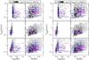 |
Fig. 7 Period–mass density distribution of present-day WD+MS PCEBs for two of our four best models (gray scale) compared with the observational distribution (magenta and blue squares). The blue squares denote those systems for which the effective temperature of the WD is lower than 12 000 K, in which case the mass determination of the WD could be problematic. The top panels show the population of WD+MS PCEBs containing C/O or O/Ne WDs, middle panels are for systems containing a He WD, and the bottom ones show the entire population of WD+MS PCEBs simulated. |
Figure 7 shows the period-mass distributions of the simulated PCEBs for two of our best models (αCE = 0.3 and n(q) ∝ q) without and with including internal energy (αint = 0.0 and αint = 0.1, left and right, respectively). For each model the lefthand panels show the distribution of orbital periods as a function of the WD mass, while the right-hand panels show the same distribution as a function of the mass of the secondary. As in Fig. 6 the top panels show the sub-population of systems containing C/O or O/Ne WDs, the middle panels those with He WDs, and the bottom panels show the distributions for the entire population. We show using different symbols those WD+MS systems for which the uncertainty in the mass determination of the WD is small enough to differentiate between C/O or O/Ne WDs, and He-core WDs, and those which have effective temperatures below 12 000 K, in which case the mass determination could be problematic. We note that in the observed sample there are four WDs with undetermined masses, 15 WDs with He cores, none of which has an effective temperature below 12 000 K, and 34 systems hosting a C/O or O/Ne WD, of which eight have effective smaller than 12 000 K. Additionally, there are four binary systems for which the mass of the secondary remains unknown. Consequently, the number of observed data points is different for each of the panels of Fig. 7.
Clearly, our simulations match the observed distribution of WD+MS PCEBs remarkably well. It is interesting to note that the WD+MS binary systems that contain a He WD (middle panels of Fig. 7) occupy a narrow strip in WD masses and, moreover, the periods of these systems cluster around 0.2–0.3 days. All this is in excellent agreement with the properties of the observed subpopulation of WD+MS PCEBs with He WDs. For those WD+MS binaries containing C/O or O/Ne WDs (top panels of Fig. 7), the distribution of WD masses is considerably broader, and most of the WD masses of our synthetic subpopulation are below 1.1 M⊙, hence are C/O WDs. Our simulations also predict that WD+MS PCEBs containing an O/Ne WD are possible, although these systems should be rare, especially when no internal energy is included. This is again consistent with the observed sample, where only two systems contain an O/Ne WD. The periods of WD+MS PCEBs with C/O or O/Ne WDs also span a wider range, with typical periods ranging from ≤0.1 to about four days, also in good agreement with the observations. When all the WD+MS PCEBs with available period and masses are considered (bottom panels), the agreement with the observed distribution is excellent.
6. Conclusions
In this paper we presented a comprehensive set of Monte Carlo simulations of the population of WD+MS PCEBs in the SDSS. Our simulations encompass a very broad range of possible situations, including three IMRDs, and different prescriptions for the treatment of the CE episode and of the parameters controlling the tidally enhanced mass loss during this phase. In our simulations we included all the known systematic observational biases. We found that the color cuts reduce the initial sample considerably and that typically only ∼7% of the simulated WD+MS PCEBs survive the cuts. The number of surviving systems is further reduced when the spectroscopic completeness filter is applied, leaving only ∼3% of the systems that previously survived the color cuts. The intrinsic binary bias and the period filter additionally reduce the total size of the simulated samples, resulting in total sample sizes that are ∼0.1% of the initial one. All in all, our simulations show that, given the actual observational capabilities, we are probing a very limited number of WD+MS PCEBs and that the observed sample suffers from low-quality statistics. This prevents drawing definite conclusions about the overall properties of the WD+MS PCEB population, despite the strong observational efforts done so far. Additionally, we find that the population of WD+MS PCEBs containing He WDs is over-represented within SDSS due to selection effects.
Nevertheless, a comparison of our population synthesis simulations with the complete sample of PCEBs currently available allowed us to draw some interesting conclusions, although we emphasize that to reach physically sound conclusions, the theoretical results can only be compared with observations once all the observational selection effects are properly taken into account. Thus, in this paper we simulated for the first time the entire process of discovery, PCEB identification, and orbital period determination of PCEBs discovered by SDSS and compared model predictions and observations. Our results can be summarized as follows:
-
Even for low values of the mass-loss enhancement parameter, thepercentage of He WDs is at odds with what is foundobservationally. Low values of this parameter agree better withthe observational data set.
-
A low value of the CE efficiency (αCE ≤ 0.3) is required to reproduce the observed number of PCEBs containing He-core WDs.
-
An interesting feature of our synthetic distributions is also the resulting large fraction of He WDs in several of the theoretical distributions. Even our best-fit models have on average He WD fractions greater than those observationally found, although they agree within the error bars with the observed value. We judge that this issue is a potentially interesting feature that might be real. However, the existence of this feature deserves further study from both the theoretical and observational sides.
-
Models with a variable binding energy parameter seem to fit the observed distribution of periods better than models in which the binding energy parameter is assumed to be constant.
-
Our results also show that high values of αint are ruled out by the observations, although the ensemble properties of the population of WD+MS PCEBs do not allow us to discard low values of αint, say less than 0.2, approximately.
-
We also compared the distribution of orbital periods as a function of the mass and find excellent agreement with the observational data. Our simulations are able to reproduce not only the distribution of orbital periods, but also the observed period distribution as a function of the mass of the WD if low values for the CE efficiencies and a detailed prescription of the binding energy parameter are assumed.
Finally, we note that the present analysis suffers from the still small number of WD+MS PCEBs that have been identified in a homogenous way. This prevents us from drawing more definite conclusions. However, evidence for small CE efficencies is building up.
Acknowledgments
This research was supported by AGAUR, by MCINN grant AYA2011-23102, by the European Union FEDER funds, by the ESF EUROGENESIS project, by AECI grant A/023687/09, and by Fondecyt (grants 3110049 and 3130559). M.R.S. thanks the Millennium Science Initiative, Chilean Ministry of Economy, Nucleus P10-022-F. Part of the the research leading to these results has received funding from the European Research Council under the European Union’s Seventh Framework Program (FP/2007-2013/ERC Grant Agreement No. 320964, WDTracer). B.T.G. was supported in part by the UK=92s Science and Technology Facilities Council (ST/I001719/1). A.R.M. acknowledges financial support from the Postdoctoral Science Foundation of China (grant 2013M530470) and from the Research Fund for International Young Scientists by the National Natural Science Foundation of China (grant 11350110496).
References
- Abazajian, K. N., Adelman-McCarthy, J. K., &Agüeros, M. A., et al. 2009, ApJS, 182, 543 [NASA ADS] [CrossRef] [Google Scholar]
- Althaus, L. G.,García-Berro, E.,Isern, J., &Córsico, A. H. 2005, A&A, 441, 689 [NASA ADS] [CrossRef] [EDP Sciences] [Google Scholar]
- Althaus, L. G.,García-Berro, E.,Isern, J.,Córsico, A. H., &Rohrmann, R. D. 2007, A&A, 465, 249 [NASA ADS] [CrossRef] [EDP Sciences] [Google Scholar]
- Bochanski, Jr., J. J. 2008, Ph.D. Thesis, University of Washington, USA [Google Scholar]
- Bochanski, J. J.,Hawley, S. L., &West, A. A. 2011, AJ, 141, 98 [NASA ADS] [CrossRef] [Google Scholar]
- Catalán, S.,Isern, J.,García-Berro, E., &Ribas, I. 2008, MNRAS, 387, 1693 [NASA ADS] [CrossRef] [Google Scholar]
- Chernick, M. 2007, Bootstrap methods: A guide for practitioners and researchers (Wiley-Interscience), 619 [Google Scholar]
- Davis, P. J.,Kolb, U., &Willems, B. 2010, MNRAS, 403, 179 [NASA ADS] [CrossRef] [Google Scholar]
- de Kool, M. 1990, ApJ, 358, 189 [NASA ADS] [CrossRef] [Google Scholar]
- de Kool, M. 1992, A&A, 261, 188 [NASA ADS] [Google Scholar]
- De Marco, O.,Passy, J.-C.,Moe, M., et al. 2011, MNRAS, 411, 2277 [NASA ADS] [CrossRef] [Google Scholar]
- Dewi, J. D. M., &Tauris, T. M. 2000, A&A, 360, 1043 [NASA ADS] [Google Scholar]
- Eggleton, P. P. 1983, ApJ, 268, 368 [NASA ADS] [CrossRef] [Google Scholar]
- Frieman, J. A., Bassett, B., &Becker, A., et al. 2008, AJ, 135, 338 [Google Scholar]
- García-Berro, E.,Torres, S.,Isern, J., &Burkert, A. 1999, MNRAS, 302, 173 [NASA ADS] [CrossRef] [Google Scholar]
- García-Berro, E.,Torres, S.,Isern, J., &Burkert, A. 2004, A&A, 418, 53 [NASA ADS] [CrossRef] [EDP Sciences] [Google Scholar]
- Hakkila, J.,Myers, J. M.,Stidham, B. J., &Hartmann, D. H. 1997, AJ, 114, 2043 [NASA ADS] [CrossRef] [Google Scholar]
- Han, Z.,Podsiadlowski, P., &Eggleton, P. P. 1995, MNRAS, 272, 800 [NASA ADS] [Google Scholar]
- Heggie, D. C. 1975, MNRAS, 173, 729 [NASA ADS] [CrossRef] [Google Scholar]
- Heller, R.,Homeier, D.,Dreizler, S., &Østensen, R. 2009, A&A, 496, 191 [NASA ADS] [CrossRef] [EDP Sciences] [Google Scholar]
- Holmberg, J., &Flynn, C. 2000, MNRAS, 313, 209 [NASA ADS] [CrossRef] [Google Scholar]
- Hurley, J. R.,Pols, O. R., &Tout, C. A. 2000, MNRAS, 315, 543 [NASA ADS] [CrossRef] [Google Scholar]
- Hurley, J. R.,Tout, C. A., &Pols, O. R. 2002, MNRAS, 329, 897 [NASA ADS] [CrossRef] [Google Scholar]
- James, F. 1990, Comput. Phys. Commun., 60, 329 [NASA ADS] [CrossRef] [Google Scholar]
- Jordi, K.,Grebel, E. K., &Ammon, K. 2006, A&A, 460, 339 [NASA ADS] [CrossRef] [EDP Sciences] [Google Scholar]
- Koester, D.,Napiwotzki, R.,Voss, B.,Homeier, D., &Reimers, D. 2005, A&A, 439, 317 [NASA ADS] [CrossRef] [EDP Sciences] [Google Scholar]
- Kroupa, P.,Tout, C. A., &Gilmore, G. 1993, MNRAS, 262, 545 [NASA ADS] [CrossRef] [Google Scholar]
- Li, N., &Thakar, A. R. 2008, Comp. Sci. Eng., 10, 18 [CrossRef] [Google Scholar]
- Nebot Gómez-Morán, A., Gänsicke, B. T., &Schreiber, M. R., et al. 2011, A&A, 536, A43 [CrossRef] [Google Scholar]
- Nelemans, G., &Tout, C. A. 2005, MNRAS, 356, 753 [NASA ADS] [CrossRef] [Google Scholar]
- Nelemans, G., Yungelson, L. R., Portegies Zwart, S. F., &Verbunt, F. 2001, A&A., 365, 491 [NASA ADS] [CrossRef] [EDP Sciences] [Google Scholar]
- Politano, M., &Weiler, K. P. 2007, ApJ, 665, 663 [NASA ADS] [CrossRef] [Google Scholar]
- Press, W. H., Flannery, B. P., & Teukolsky, S. A. 1986, Numerical Recipes, The art of scientific computing (Cambridge University Press) [Google Scholar]
- Rebassa-Mansergas, A.,Gänsicke, B. T.,Rodríguez-Gil, P.,Schreiber, M. R., &Koester, D. 2007, MNRAS, 382, 1377 [NASA ADS] [CrossRef] [Google Scholar]
- Rebassa-Mansergas, A.,Gänsicke, B. T.,Schreiber, M. R., et al. 2008, MNRAS, 390, 1635 [NASA ADS] [Google Scholar]
- Rebassa-Mansergas, A.,Gänsicke, B. T.,Schreiber, M. R.,Koester, D., &Rodriguez-Gil, P. 2010, MNRAS, 406, 620 [NASA ADS] [CrossRef] [Google Scholar]
- Rebassa-Mansergas, A., Nebot Gómez-Morán, A.,Schreiber, M. R.,Girven, J., &Gänsicke, B. T. 2011, MNRAS, 413, 1121 [NASA ADS] [CrossRef] [Google Scholar]
- Rebassa-Mansergas, A., Nebot Gómez-Morán, A.,Schreiber, M. R., et al. 2012, MNRAS, 419, 806 [NASA ADS] [CrossRef] [Google Scholar]
- Rebassa-Mansergas, A.,Agurto-Gangas, C.,Schreiber, M. R.,Gänsicke, B. T., &Koester, D. 2013, MNRAS, 433, 3398 [NASA ADS] [CrossRef] [Google Scholar]
- Reimers, D., &Kudritzki, R. P. 1978, A&A, 365, 227 [Google Scholar]
- Renedo, I., Althaus, L. G., Miller Bertolami, M. M., et al. 2010, ApJ, 717, 183 [NASA ADS] [CrossRef] [Google Scholar]
- Richards, G. T., Fan, X., Newberg, H. J., et al. 2002, AJ, 123, 2945 [NASA ADS] [CrossRef] [Google Scholar]
- Ricker, P. M., &Taam, R. E. 2012, ApJ, 746, 74 [NASA ADS] [CrossRef] [Google Scholar]
- Schlegel, D. J.,Finkbeiner, D. P., &Davis, M. 1998, ApJ, 500, 525 [NASA ADS] [CrossRef] [Google Scholar]
- Schreiber, M. R., &Gänsicke, B. T. 2003, A&A, 406, 305 [NASA ADS] [CrossRef] [EDP Sciences] [Google Scholar]
- Schreiber, M. R., Gänsicke, B. T., & Rebassa-Mansergas, A., et al. 2010, VizieR Online Data Catalog, J/A+A/513/L7 [Google Scholar]
- Serenelli, A. M.,Althaus, L. G.,Rohrmann, R. D., &Benvenuto, O. G. 2001, MNRAS, 325, 607 [NASA ADS] [CrossRef] [Google Scholar]
- Smolčić, V., Ivezić, Ž., & Knapp, G. R., et al. 2004, ApJ, 615, L141 [NASA ADS] [CrossRef] [Google Scholar]
- Strauss, M. A., Weinberg, D. H., &Lupton, R. H., et al. 2002, AJ, 124, 1810 [NASA ADS] [CrossRef] [Google Scholar]
- Taam, R. E., &Ricker, P. M. 2010, New Astron. Rev., 54, 65 [NASA ADS] [CrossRef] [Google Scholar]
- Toonen, S., &Nelemans, G. 2013, A&A, 557, A87 [NASA ADS] [CrossRef] [EDP Sciences] [Google Scholar]
- Tout, C. A., &Eggleton, P. P. 1988, MNRAS, 231, 823 [NASA ADS] [CrossRef] [Google Scholar]
- Vassiliadis, E., &Wood, P. R. 1993, ApJ, 413, 641 [NASA ADS] [CrossRef] [Google Scholar]
- Webbink, R. F. 1984, ApJ, 277, 355 [NASA ADS] [CrossRef] [Google Scholar]
- West, A. A.,Hawley, S. L.,Bochanski, J. J., et al. 2008, AJ, 135, 785 [NASA ADS] [CrossRef] [Google Scholar]
- West, A. A.,Morgan, D. P.,Bochanski, J. J., et al. 2011, AJ, 141, 97 [NASA ADS] [CrossRef] [Google Scholar]
- Willems, B., &Kolb, U. 2004, A&A, 419, 1057 [NASA ADS] [CrossRef] [EDP Sciences] [Google Scholar]
- Yanny, B.,Rockosi, C.,Newberg, H. J., et al. 2009, AJ, 137, 4377 [NASA ADS] [CrossRef] [Google Scholar]
- Zorotovic, M., Schreiber, M. R., Gänsicke, B. T., & Nebot Gómez-Morán, A. 2010, A&A, 520, A86 [NASA ADS] [CrossRef] [EDP Sciences] [Google Scholar]
- Zorotovic, M.,Schreiber, M. R.,Gänsicke, B. T., et al. 2011, A&A, 536, L3 [NASA ADS] [CrossRef] [EDP Sciences] [Google Scholar]
All Tables
Total number and percentage of simulated WD+MS binary systems obtained after applying the successive selection criteria.
Enhanced mass-loss parameter and percentage of PCEBs with different types of WDs.
Percentage of systems with He WDs and KS test of the period distribution for six representative models with λ = 0.5.
Percentage of systems with He WDs and KS test of the period distribution for our models with αCE ≤ 0.3 and λ properly computed for each system, where different fractions of internal energy are taken into account.
All Figures
|
Fig. 1 Position of Legacy (black) and SEGUE (red) SDSS DR 7 WD+MS binaries in Galactic and equatorial coordinates. Taken from Rebassa-Mansergas et al. (2012). (Color version online.) |
| In the text | |
|
Fig. 2 Detection probability of a PCEB as a function of the orbital period. |
| In the text | |
|
Fig. 3 Color–color diagram of the synthetic WD+MS PCEBs obtained using our Monte Carlo simulator when our reference model (αCE = 1.0, λ = 0.5, and n(q) = 1) is employed. Systems containing He WDs are represented using black dots, while blue dots correspond to systems with C/O or O/Ne WDs. The observed WD+MS PCEB systems are displayed using red dots. The color selection criteria are shown using red lines (Sect. 3.1). (Color version online.) |
| In the text | |
|
Fig. 4 Color–magnitude diagram of the synthetic WD+MS PCEBs obtained using our Monte Carlo simulator (blue and black dots) compared with the observed systems (red symbols) after applying the different filters explained in the text to our reference model. Colors are the same as in Fig. 3. (Color version online.) |
| In the text | |
|
Fig. 5 From top to bottom: binding energy parameter, primary ZAMS mass, WD mass and orbital period as a function of the Roche-lobe radius of the primary, as given in Eggleton (1983). The case B, case C and TPAGB case CE episodes are represented using green, blue and red dots, respectively. The two sides show the results for two models in which αCE = 0.3 and n(q) = 1 but without and with a fraction of the internal energy contributing to expel the envelope: αint = 0.0 (left panels) and αint = 0.2 (right panels). (Color version online.) |
| In the text | |
|
Fig. 6 Period histograms (normalized to unit area) of the distribution of present-day WD+MS PCEBs for our four best models (black line) compared with the observational distribution (dotted line, gray histogram). |
| In the text | |
|
Fig. 7 Period–mass density distribution of present-day WD+MS PCEBs for two of our four best models (gray scale) compared with the observational distribution (magenta and blue squares). The blue squares denote those systems for which the effective temperature of the WD is lower than 12 000 K, in which case the mass determination of the WD could be problematic. The top panels show the population of WD+MS PCEBs containing C/O or O/Ne WDs, middle panels are for systems containing a He WD, and the bottom ones show the entire population of WD+MS PCEBs simulated. |
| In the text | |
Current usage metrics show cumulative count of Article Views (full-text article views including HTML views, PDF and ePub downloads, according to the available data) and Abstracts Views on Vision4Press platform.
Data correspond to usage on the plateform after 2015. The current usage metrics is available 48-96 hours after online publication and is updated daily on week days.
Initial download of the metrics may take a while.