| Issue |
A&A
Volume 566, June 2014
|
|
|---|---|---|
| Article Number | A87 | |
| Number of page(s) | 11 | |
| Section | Galactic structure, stellar clusters and populations | |
| DOI | https://doi.org/10.1051/0004-6361/201322919 | |
| Published online | 19 June 2014 | |
Constraining the vertical structure of the Milky Way rotation by microlensing in a finite-width global disk model⋆
1
Institute of Nuclear Physics, Polish Academy of Sciences,
Radzikowskego 152,
31342
Kraków,
Poland
e-mail:
This email address is being protected from spambots. You need JavaScript enabled to view it.
2
Astronomical Observatory, Jagellonian University,
Orla 171,
30244
Kraków,
Poland
3
Institute of Physics, Jagellonian University,
Reymonta 4,
30059
Kraków,
Poland
Received:
26
October
2013
Accepted:
24
April
2014
Abstract
We model the vertical structure of mass distribution of the Milky Way galaxy in the framework of a finite-width global disk model. Assuming only the Galactic rotation curve, we tested the predictions of the model inside the solar orbit for two measurable processes that are unrelated to each other: the gravitational microlensing that allows one to fix the disk width-scale by the best fit to measurements, and the vertical gradient of rotation modeled in the quasi-circular orbits approximation. The former is sensitive to the gravitating mass in compact objects, the latter to all kinds of gravitating matter. The analysis points to a small width-scale of the considered disks and an at-most insignificant contribution of non-baryonic dark matter in the solar circle. The predicted high vertical gradient values in the rotation are consistent with the gradient measurements.
Key words: gravitational lensing: micro / Galaxy: disk / Galaxy: kinematics and dynamics / Galaxy: structure
Appendix A is available in electronic form at http://www.aanda.org
© ESO, 2014
1. Introduction
The Milky Way (MW) is an example of a galaxy with high vertical gradients of rotation measured at low altitudes above the mid-plane (Levine et al. 2008). It is interesting to see the effect of the disk thickness on the gradient value prediction and to compare it with the analogous prediction in an infinitesimally thin global disk model (Jałocha et al. 2010).
The gravitational microlensing phenomenon provides another constraint on the mass distribution, independent of the vertical gradient structure. In particular, the amount of mass seen through the gravitational microlensing measurements inside the solar orbit was shown to be consistent with the dynamical mass ascertained from the Galactic rotation that is reduced by the gas contribution that is undetectable by the microlensing (Sikora et al. 2012).
In the present paper we use microlensing measurements to constrain the disk width and compare the resulting vertical gradient predictions with the gradient measurements. In our several previous studies, e.g., Jałocha et al. (2010, 2011), we modeled spiral galaxies in the approximation of an infinitesimally thin disk. In this framework, we easily obtained high values of the vertical gradient of rotation, in accord with gradient measurements. However, the model does not account for the vertical structure in the mass distribution in the direct neighborhood of the mid-plane (the z = 0 vicinity). This structure can be modeled by considering a finite-width disk with an assumed vertical profile of mass density. We presented a preliminary step towards this in Sikora et al. (2012), where a column mass density of a disk with the exponential vertical profile was identified with the surface density of an infinitesimally thin disk. But this was a simple de-projection that did not take into account the redistribution of mass required to preserve the shape of the rotation curve in the vicinity of the Galactic center.
In the next approximation considered in this paper, in Sects. 2 and 3, we find the volume mass densities of two example finite-width disks by iterations. These disks exactly account for the tabulated rotation curve of the MW and their width-scales are constrained by the gravitational microlensing measurements. In Sect. 4 we compare the predictions of the two models with the measurements of the vertical gradient of rotation.
2. Finite-width disk model
We assumed the following factorized form of a volume mass density ρ(r,z) =
σ(r)f(z),
with factors normalized so that σ(r) is the column mass density and
the vertical profile f(z) is integrable to unity:
 . We considered the exponential
vertical profile (for its simplicity) and the Mexican hat profile (because it is frequently
used in star count models that are motivated by Spitzer
1942 analysis):
. We considered the exponential
vertical profile (for its simplicity) and the Mexican hat profile (because it is frequently
used in star count models that are motivated by Spitzer
1942 analysis): 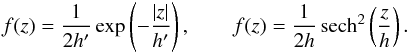 (1)The
width-scale parameters h′ and h can be related by equating
their effective disk thicknesses: 2
h′ and ≈1.49 h, respectively, defined by the
(1)The
width-scale parameters h′ and h can be related by equating
their effective disk thicknesses: 2
h′ and ≈1.49 h, respectively, defined by the
 criterion 1.
The gravitational potential at a point X = [ R,0,Z
] associated with a mass element dm = ρ(r,z)
rdr dφ
dz located at another point Y = [
rcos φ,r sin φ,z ], is
 ,
where
,
where  .
By substituting φ =
2α − π, using the symmetry
φ → −φ, integrating over
.
By substituting φ =
2α − π, using the symmetry
φ → −φ, integrating over
 and using the definition of of the elliptic integral of the first kind K (Gradshtein et al. 2007), one arrives at an expression for the total
potential Ψ(R,Z) at X:
and using the definition of of the elliptic integral of the first kind K (Gradshtein et al. 2007), one arrives at an expression for the total
potential Ψ(R,Z) at X:
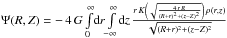 .With
the help of the identity
.With
the help of the identity 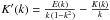 (Gradshtein et al. 2007), it can be shown that
 . Function J is an integration kernel
that will frequently appear later:
. Function J is an integration kernel
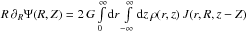
that will frequently appear later: 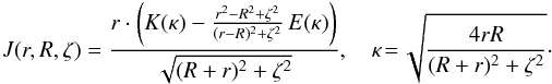 The
expression for R∂RΨ(R,Z)
can be used to compute the rotation velocity vφ(R,Z)
in the quasi-circular orbits approximation studied in Jałocha et al. (2010). In this approximation,
The
expression for R∂RΨ(R,Z)
can be used to compute the rotation velocity vφ(R,Z)
in the quasi-circular orbits approximation studied in Jałocha et al. (2010). In this approximation,
 , and the
resulting vertical gradient of rotation is ∂Zvφ(R,Z).
The latter quantity would involve differentiation of the kernel J under the integration sign.
However, since ρ(r,z) is of the form
σ(r)f(z),
with f(z) being known in an analytic form,
falling off fast enough as |z| →
∞, and satisfying the reflection symmetry f(z) = f(−z), it is more convenient to integrate by parts Noting
that ∂zJ = −∂ZJ, we
are led to the following expressions for the circular velocity and its vertical gradient (by
the assumed reflection symmetry of f, the integration has been restricted to
z>
0):
, and the
resulting vertical gradient of rotation is ∂Zvφ(R,Z).
The latter quantity would involve differentiation of the kernel J under the integration sign.
However, since ρ(r,z) is of the form
σ(r)f(z),
with f(z) being known in an analytic form,
falling off fast enough as |z| →
∞, and satisfying the reflection symmetry f(z) = f(−z), it is more convenient to integrate by parts Noting
that ∂zJ = −∂ZJ, we
are led to the following expressions for the circular velocity and its vertical gradient (by
the assumed reflection symmetry of f, the integration has been restricted to
z>
0):  (The
derivatives of J have been eliminated from Eq. (3) by means of an integration by parts.) We
stress that these two expressions are only valid in the quasi-circular orbit approximation.
(The
derivatives of J have been eliminated from Eq. (3) by means of an integration by parts.) We
stress that these two expressions are only valid in the quasi-circular orbit approximation.
The above integral expressions are particularly suited for the exponential vertical
profile, in which case they reduce to  and
and
 ,
where I− and I+ are appropriate
integrals involving J(r,R,z − Z) and
J(r,R,z +
Z), respectively.
,
where I− and I+ are appropriate
integrals involving J(r,R,z − Z) and
J(r,R,z +
Z), respectively.
For a more explicit derivation of the above results, we refer to the appendix.
2.1. Determining ρ(r,z) from the rotation curve by iterations
We used the smoothed-out MW rotation curve from Sofue et al. (1999), which adopts Galactic constants Ro = 8 kpc and Ωo = 200 km s-1. Its inner part, inside the solar circle, which is of interest in our paper, is relatively well determined and was obtained by simple averaging of various CO and HI tangent velocity data.The uncertainty lies mostly in the velocity parameter of the standard of rest at the Sun position, Ωo, and the radius of solar orbit Ro. For larger radii, outside the region of our interest, the rotation curve is less certain and even model dependent. Furthermore, as follows from the analysis in Bratek et al. (2008), the uncertainty in the external rotation curve implies some uncertainty in the internal mass determination because of a backward-interaction characteristic of flattened mass distributions. However, in Sikora et al. (2012) we found this influence to be marginal for the purpose of the present study. It is more important to reduce the uncontrolled numerical errors that arise because of singular kernels in integrals Eqs. (2) and (3). To achieve this, we applied a cubic spline interpolation to the rotation points. This way we obtain a continuously differentiable interpolating rotation curve (see Fig. 1).
We obtain a primary approximation to the column mass density, σ0(R), from the
interpolating rotation curve in the infinitesimally thin global disk model by iterations
similar to those described in Jałocha et al.
(2008), with the help of the following integral transforms, which are mutual
inverses of each other (Sikora et al. 2012),
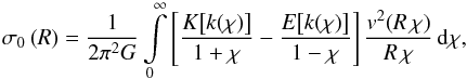 (4)and
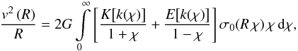 (5)with
 in both cases. The transforms relate the rotation law in the galactic mid-plane to the
surface mass density in that plane. Here, R is the radial variable in the disk plane,
K and
E are
complete elliptic integrals of the first and second kind as defined in Gradshtein et al. (2007), and χ is a dimensionless
integration variable. The surface mass density σ0(r) obtained this way
gives a primary approximation ρ0(r,z) =
σ0(r)f(z)
of the volume mass density, which should be close to the mass density in a finite-width
disk (the results of Sikora et al. (2012) were
based on this approximation). But evaluating integral Eq. (2) with ρ0(r,z) substituted for
ρ(r,z), gives a
in both cases. The transforms relate the rotation law in the galactic mid-plane to the
surface mass density in that plane. Here, R is the radial variable in the disk plane,
K and
E are
complete elliptic integrals of the first and second kind as defined in Gradshtein et al. (2007), and χ is a dimensionless
integration variable. The surface mass density σ0(r) obtained this way
gives a primary approximation ρ0(r,z) =
σ0(r)f(z)
of the volume mass density, which should be close to the mass density in a finite-width
disk (the results of Sikora et al. (2012) were
based on this approximation). But evaluating integral Eq. (2) with ρ0(r,z) substituted for
ρ(r,z), gives a
 different from
  by a small amount
 measuring the discrepancy
between the predicted and the observed rotation. Now, by inserting the
measuring the discrepancy
between the predicted and the observed rotation. Now, by inserting the
 in place of v2 in Eq. (4), we obtain a correction Δσ0(R) to the column mass
density. Hence, the surface mass density in the next approximation is2σ1(R) =
σ0(R) +
λ·Δσ0(R)
and gives rise to a corrected volume mass density ρ1(r,z) =
σ1(r)f(z),
which in turn, from Eq. (2), gives the
corresponding corrected rotation curve vφ,1(R,0).
Next, we shift all indices by +1 and repeat the previous step. This correction process can be
continued recursively until it converges to the desired density profile ρ(r,z) for
which the discrepancy
in place of v2 in Eq. (4), we obtain a correction Δσ0(R) to the column mass
density. Hence, the surface mass density in the next approximation is2σ1(R) =
σ0(R) +
λ·Δσ0(R)
and gives rise to a corrected volume mass density ρ1(r,z) =
σ1(r)f(z),
which in turn, from Eq. (2), gives the
corresponding corrected rotation curve vφ,1(R,0).
Next, we shift all indices by +1 and repeat the previous step. This correction process can be
continued recursively until it converges to the desired density profile ρ(r,z) for
which the discrepancy  becomes
negligible. The resulting recursion sequence of volume densities ρj(R,Z) =
ρj−1(R,Z) +
λ·f(Z)Δσj
− 1(R) is quickly converging to a limit
ρ(R,Z) =
limj →
∞ρj(R,Z)
which, on substituting to Eq. (2), yields a
curve vφ(R,0)
that nicely overlaps the interpolating rotation curve. The iteration process is
illustrated in Fig. 1.
becomes
negligible. The resulting recursion sequence of volume densities ρj(R,Z) =
ρj−1(R,Z) +
λ·f(Z)Δσj
− 1(R) is quickly converging to a limit
ρ(R,Z) =
limj →
∞ρj(R,Z)
which, on substituting to Eq. (2), yields a
curve vφ(R,0)
that nicely overlaps the interpolating rotation curve. The iteration process is
illustrated in Fig. 1.
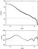 |
Fig. 1 Column mass densities and the corresponding rotation curves of finite-width disks with a Mexican hat vertical profile (h = 117 pc), shown at several steps of the iteration method of Sect. 2.1, starting from the surface density of an infinitesimally thin disk. Top panel: column mass densities at various iteration steps (thin gray lines), surface mass density of the infinitesimally thin disk model (the starting point of the iteration, triangles), MW column mass density in the final iteration step (it gives the interpolating rotation curve in the bottom panel, solid circles). Bottom panel: (open circles) MW rotation curve points from Sofue et al. (1999), (thin gray lines) rotation curves at various iteration steps, and (thick line) rotation curve in the final iteration step (it strictly overlaps with a spline interpolation of the MW rotation curve points). |
In Sect. 3 we use this method of finding column mass densities σ(R) corresponding to various vertical profiles f(z). They all give rise to rotation laws that overlap in the mid-plane the MW rotation curve.
3. Gravitational microlensing
The phenomenon of the gravitational light deflection in point mass fields, called gravitational microlensing, may be used to trace the mass distribution. This can be achieved by inferring the amount of mass in compact objects scattered along various lines of sight that join the observer and remote sources of light that are distributed in the vicinity of the Galactic center. Because it is not directly linked to the Galaxy dynamics, the gravitational microlensing provides an independent tool that is useful in testing Galactic models.
The original idea comes from Paczynski (1986), who suggested that gravitational lensing can be used to answer the question of whether or not the spheroidal component of the Galaxy is dominated by massive compact objects. Observations towards Great and Small Magellanic Clouds, e.g., Alcock et al. (2000); Wyrzykowski et al. (2011), indicated that the contribution from such objects cannot dominate in the standard three-component Galactic model. On the other hand, the microlensing method can also be used to estimate the distribution of compact objects in the direction towards the Galactic center. Such measurements can help to improve models of the Galactic interior, see e.g., Bissantz et al. (2004). It should be pointed out that in most of these models, the dark matter component becomes necessary only beyond some particular distance from the Galactic center. For example, in the model by Bissantz & Gerhard (2002), the dark matter halo is irrelevant for distances smaller than 5 kpc from the center.
The aim of the present work is to examine in the context of the microlensing observations a Galactic model in which the dynamics is dominated by baryonic matter distributed in direct neighborhood of the Galactic mid-plane.
3.1. Optical depth
The most important quantity to be determined in the microlensing method is the optical
depth τ. It
is defined as the probability of finding a compact object (a lens) on the line of sight
between the observer and the source of light, when a lens is located within its Einstein
radius 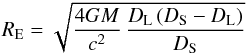 on
a plane perpendicular to the line of sight. Here, M denotes the lens mass,
DS is the distance from the observer to
the source, and DL is the distance between the observer
and the lens. In this particular configuration, a double image of the source is produced
each time a lens passes between the source and the observer. Although the two images
cannot usually be resolved because of very small deflection angles, their appearance can
still be indirectly detected by measuring the associated image magnification. A
microlensing event of this kind is agreed to have been occurred when the magnification
exceeds a threshold value of μ
= 1.34. Because the probability of microlensing events is very low (on
the order of 10-6),
a great number of sources (about a million) must be monitored during a period of a few
years to determine the optical depth. A detailed discussion of such observations and their
theoretical description can be found in Moniez
(2010).
on
a plane perpendicular to the line of sight. Here, M denotes the lens mass,
DS is the distance from the observer to
the source, and DL is the distance between the observer
and the lens. In this particular configuration, a double image of the source is produced
each time a lens passes between the source and the observer. Although the two images
cannot usually be resolved because of very small deflection angles, their appearance can
still be indirectly detected by measuring the associated image magnification. A
microlensing event of this kind is agreed to have been occurred when the magnification
exceeds a threshold value of μ
= 1.34. Because the probability of microlensing events is very low (on
the order of 10-6),
a great number of sources (about a million) must be monitored during a period of a few
years to determine the optical depth. A detailed discussion of such observations and their
theoretical description can be found in Moniez
(2010).
The principle result of the microlensing theory is the following integral that relates
the mass density of compact objects ρ(x) and the optical
depth τ:
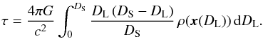 (6)Although
it is well known, we re-derived this formula for completeness in our previous paper (Sikora et al. 2012). The integration in Eq. (6) is carried out along a given line of sight
between the observer’s position x⊙ = [Ro,0,0] and the source of light located at x⊗ =
x⊙ + (1 +
χ)Ro [−cos bcos l, −cos b sin l, sin b].
The angle l
is the Galactic longitude, b is the Galactic latitude, and χ is a dimensionless
distance parameter, such that DS = Ro (1 +
χ). Using the following parameterization of the line
of sight x(s) =
x⊙ + s
(x⊗ −
x⊙), Eq. (6) can be rewritten such that τ becomes an explicit
function of the source position (l,b,χ) (Sikora et
al. 2012),
(6)Although
it is well known, we re-derived this formula for completeness in our previous paper (Sikora et al. 2012). The integration in Eq. (6) is carried out along a given line of sight
between the observer’s position x⊙ = [Ro,0,0] and the source of light located at x⊗ =
x⊙ + (1 +
χ)Ro [−cos bcos l, −cos b sin l, sin b].
The angle l
is the Galactic longitude, b is the Galactic latitude, and χ is a dimensionless
distance parameter, such that DS = Ro (1 +
χ). Using the following parameterization of the line
of sight x(s) =
x⊙ + s
(x⊗ −
x⊙), Eq. (6) can be rewritten such that τ becomes an explicit
function of the source position (l,b,χ) (Sikora et
al. 2012), 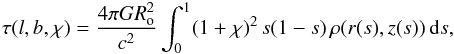 (7)where
![Mathematical equation: \hbox{$r(s)=\rsun\,\sqrt{1+s\,(1+\chi)\cos b\,\left[s\,(1+\chi)\cos b-2\cos l \right]}$}](/articles/aa/full_html/2014/06/aa22919-13/aa22919-13-eq95.png) and z(s) =
Ros (1 +
χ)sinb. Given a density
distribution ρ(r,z), the above formula enables
one to calculate the corresponding optical depth.
and z(s) =
Ros (1 +
χ)sinb. Given a density
distribution ρ(r,z), the above formula enables
one to calculate the corresponding optical depth.
3.2. Data
The model optical depth, calculated with the help of Eq. (7), must be compared with the observations. For that purpose, we used data collected by several leading collaborations, in particular MACHO (Popowski et al. 2005), EROS (Hamadache et al. 2006), OGLE (Sumi et al. 2006), and MOA (Sumi & et al. 2003). These data were collected and analysed in detail in a review (Moniez 2010).
Below, we restrict our analysis to the bright stars subsample. This is a commonly used strategy in minimizing blending processes that affect the optical depth results. A discussion of the blending effect can be found in Alard (1997) and Smith et al. (2007). The data we used are represented as a function of latitude τ(b), and for each b the optical depth was averaged over the longitudinal angle in the interval l ∈ (−5°,5°). The resulting function τ(b) allows us to study the vertical structure of the Galaxy.
3.3. Previous results in view of the present study
In our previous paper (Sikora et al. 2012), we used a surface mass density σ(r) that accounts for the Galactic rotation curve in the infinitesimally thin disk model to obtain a volume mass density ρ(r,z) corresponding to σ(r), assuming the standard exponential vertical profile ρ(r,z) = ρ(r,0) e−| z | /h′. Following the EROS collaboration, e.g., Derue et al. (2001), we set the value of the width-scale parameter to be h′ = 325 pc. With this ρ(r,z) we showed that the resulting optical depth was consistent with the observational data at a reasonable confidence level. In addition, we investigated several problems that might influence the optical depth, among them the uncertainty of the solar Galacto-centric distance Ro, the problem of a precise determination of the rotation curve, the difference between a single exponential vertical profile and a double exponential profile, and the structure of the central bulge. We pointed out that the optical depth uncertainty connected with each of these factors was relatively small and could not spoil the consistency between the model predictions and the observations.
The purpose of the present work is to check the microlensing optical depth predictions within a finite-width disk model framework, assuming a spatial mass distribution derived directly from the interpolating rotation curve, as described in Sect. 2.1. In this model the disk thickness is crucial and affects the distribution of column mass density, which can change, while keeping the predicted rotation unchanged and identical with the interpolating rotation curve of Sect. 2.1. As mentioned earlier, we assumed a volume mass density of the form ρ(r,z) = σ(r)f(z), where σ(r) is the column mass density and f(z) is either the normalized Mexican hat or exponential vertical profiles given in Eq. (1). Each of these profiles is defined by its own characteristic width-scale, h or h′, which are free parameters. Their optimal values can be constrained with the help of microlensing measurements, as we show in the next subsection.
3.4. Microlensing in a finite-width disk model
The sources of light observed in the microlensing events are randomly distributed in the vicinity of the Galactic center. This requires some averaging in the latitudinal angle b. Hence, the optical depth observable (as a function of b) should be understood as a moving average. It is frequently assumed that the sources are located on the symmetry axis. We adopted this simplification in calculating τ(b) by substituting l = 0 and χ = 0 in Eq. (7).
Our idea of determining τ(b) is simple. For a fixed width-scale h or h′, we obtain a volume mass density ρ(r,z) from the Galactic rotation curve, as described in detail in Sect. 2.1. With this ρ(r,z) we calculate the optical depth τ(b) from Eq. (7), substituting l = 0 and χ = 0. The results for the vertical density profiles Eq. (1) are shown in Figs. 2 and 3. The curves, corresponding to different width-scale values, are shown together with the observed data points described in Sect. 3.2. We recall that we are only interested in the bright stars subsample.
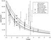 |
Fig. 2 Optical depth τ(b) in the finite-width disk model for the Mexican hat vertical profile, with the width-scales (1) h = 180 pc; (2) h = 150 pc; (3) h = 117 pc /the best fit/; and (4) h = 100 pc (solid lines). The points with error bars represent the measurement data collected by several collaborations (references in the text). |
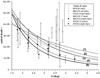 |
Fig. 3 Optical depth τ(b) in the finite-width disk model for the exponential vertical profile with the width-scales (1) h′ = 325 pc; (2) h′ = 200 pc; (3) h′ = 150 pc; (4) h′ = 100 pc; (5) h′ = 88 pc /the best fit/ (solid lines). For comparison, the thick gray line represents the τ(b) in the infinitesimally thin disk model for which the equivalent volume mass density was obtained assuming the exponential vertical profile with h′ = 325 pc. The points with error bars represent measurements data collected by several collaborations (references in the text). |
To measure the accuracy of the fitting curves obtained for various width-scales, we
calculated the reduced chi-squared,  , that is, the
chi-squared divided by the number of the degrees of freedom (the fit residuals from the
bright stars subsample were taken into account). The
are plotted
in Fig. 4 for several width-scales h (black dots in the top
panel) and h′ (black dots in the bottom panel). By
cubic-spline-interpolating the , we may
regard it as a smooth function of the width-scale. This allows us to determine the optimum
width-scale at the minimum of each . The
width-scales obtained this way are h = 117 pc and h′ = 88 pc for
the Mexican hat and the exponential vertical profiles.
, that is, the
chi-squared divided by the number of the degrees of freedom (the fit residuals from the
bright stars subsample were taken into account). The
are plotted
in Fig. 4 for several width-scales h (black dots in the top
panel) and h′ (black dots in the bottom panel). By
cubic-spline-interpolating the , we may
regard it as a smooth function of the width-scale. This allows us to determine the optimum
width-scale at the minimum of each . The
width-scales obtained this way are h = 117 pc and h′ = 88 pc for
the Mexican hat and the exponential vertical profiles.
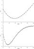 |
Fig. 4 Reduced chi-squared, |
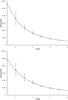 |
Fig. 5 Results of a Monte Carlo simulation: the mean optical depth and its standard deviation for a sample of sources chosen randomly with a probability distribution proportional to ρ(r,z), (points+error bars). For comparison, the (solid line) shows the optical depth calculated with the help of the integral of Eq. (7) with l = 0 and χ = 0. Top panel: results for the Mexican hat vertical profile with h = 117 pc. Bottom panel: results for the exponential vertical profile with h′ = 88 pc. |
Finally, we need to verify whether the approximation of sources aligned with the symmetry axis is justified. To this end we performed a Monte Carlo simulation. We randomly chose a number of n = 104 pairs (l,χ) in the range χ ∈ (−0.125,0.125) (corresponding to ± 1 kpc) and l ∈ (−5°,5°) for each fixed latitude b, with the probability weight directly proportional to ρ(r,z), simultaneously finding the corresponding τ(l,b,χ) as defined in Eq. (7). The resulting mean optical depth and its standard deviation are shown as functions of b in Fig. 5. The mean value is close to τ(0,b,0) (solid line), which proves the approximation to be quite accurate.
4. Vertical gradient of rotation
In Jałocha et al. (2010) we modeled the vertical gradient of the MW rotation in the framework of the infinitesimally thin disk model. We compared the predicted high absolute gradient values with the gradient measurements by Levine et al. (2008) and found them to be consistent. In what follows, we repeat these studies in a more accurate model that accounts for a finite disk thickness, to see the influence of the vertical structure of mass distribution on the gradient value and its behavior.
The microlensing results of Sect. 3.4 imply a
width-scale of 117 pc for the
disk with the Mexican hat vertical profile, and 88 pc for that with the exponential vertical profile. With the
corresponding mass distributions substituted in Eq. (3), we find our prediction for the vertical gradient of rotation in the
rectangular measurement region of Levine et al.
(2008):  and
and
 .
Our predictions for the gradient in this region are shown in Fig. 10, where they are also compared with the predictions of the
infinitesimally thin disk model and with those of finite-width disks with the exponential
vertical profile.
.
Our predictions for the gradient in this region are shown in Fig. 10, where they are also compared with the predictions of the
infinitesimally thin disk model and with those of finite-width disks with the exponential
vertical profile.
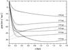 |
Fig. 6 Vertical gradient of rotation in finite-width disk models as a function of altitude above the mid-plane z = 0, shown at various radii: gradient for a disk with the Mexican hat vertical profile (h = 117 pc, solid lines), and gradient for a disk with the exponential vertical profile (h′ = 88 pc, dashed lines). To emphasize the universal gradient behavior at higher altitudes for various disks of the same mass, the results for an infinitesimally thin disk model (with the surface mass density identified with the column mass density of the disk with the Mexican hat vertical profile) is shown (dotted lines). |
For all finite-width disks, the gradient falls off to 0 at z = 0, owing to the smoothness and z-reflection symmetry of the mass distribution (then, the gradient is z-antisymmetric), while for the infinitesimally thin disk with a mass distribution singular on the symmetry plane, the gradient attains a finite and high value at z = 0 (this requires the gradient line to be discontinuous at z = 0). For low altitudes, the gradient behavior is dependent on the particular structure of mass distribution decided by the parameter h, which introduces a characteristic length that scales: the altitudinal extent of the “turn-overs” (seen in the gradient lines with h > 0), their local minimum positions, and the degree of their curvatures. Another feature evident from Fig. 10 is the fact that there is little difference between disk models with the exponential and with the Mexican hat vertical profile.
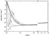 |
Fig. 7 Vertical gradient of rotation in a finite-width disk model with the Mexican hat vertical profile (solid lines), as a function of the altitude above the mid-plane (z = 0), shown at r = 4 kpc for various width-scales h. For comparison, the (dotted line) shows the gradient behavior in the limit of the infinitesimally thin disk model (h → 0). The convergence on that limit is point-wise continuous, although not uniform – the gradient for h = 0 is discontinuous at z = 0. For higher altitudes, the gradient behavior is universal beyond the main concentration of masses. |
Figure 7 shows the behavior of the gradient as a function of z at r = 4 kpc for the Mexican hat profile with various width-scales h. The smaller h, the higher the absolute value of the gradient, but the gradient is almost independent of h already for |z| > 0.4 kpc. For all finite-width disk, the smaller the width-scale, the lower the altitude above the mid-plane at which the high gradient values characteristic of the infinitesimally disk are obtained. With increasing and large enough z, the gradient in finite-width disks gradually overlaps that of the infinitesimally thin disk. For sufficiently large |z|, the differences between the predictions for disks with various h cease to be visible and a universal asymptotics can be seen. (Note that the total disk mass depends on h, which explains the tiny differences in the asymptotics, which could be formally eliminated by rescaling masses of all disks to the same value.) Physically, this behavior is clear: for high enough altitudes, the gravitational field of the infinitesimally thin disk of comparable mass perfectly approximates that of a finite-width disk beyond the main concentration of mass in the mid-plane vicinity. Mathematically, this behavior becomes clear by examining the asymptotics of the integral Eq. (3), as shown in the appendix.
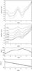 |
Fig. 8 Vertical gradient of rotation of MW in a finite-width disk model with a Mexican hat vertical profile as a function of the radial variable, shown for various width-scales h and altitudes z above the mid-plane. Top panel: gradient at an altitude of 100 pc; – h = 100 pc (dashed line), – h = 117 pc (solid line), and h = 150 pc (uppermost dash-dotted line). (For comparison, the (dash-dotted line) in the middle shows the gradient in a disk model with the vertical exponential profile and the width-scale h′ = 88 pc at the same altitude.) Upper middle panel: vertical gradient of rotation at various altitudes for h = 117 pc. To enable the comparison of structures in the vertical gradient with those in the rotation curve and in the column mass density, Lower middle panel: MW rotation curve, and bottom panel: column mass density for a finite-width disk model with a Mexican hat vertical profile (h = 117 pc). |
To understand the behavior of the gradient lines, it is useful to remember that the infinitesimally thin disk can be considered as a limit h → 0 of finite-width disks of various vertical profiles. This property is readily seen in Fig. 7. The gradient lines of finite-width disks converge point-wise on the gradient lines of the infinitesimally thin disk, although this convergence is not uniform. Owing to this fact, the gradient lines of finite-width disks are globally continuous, but there is a discontinuity at z = 0 in the gradient lines for the infinitesimally thin disk. From this convergence and the universal asymptotics referred to above, one can also infer the presence of the turn-overs of the gradient lines for finite-width disks (the reason is given in the appendix).
Figure 8 shows the gradient as a function of radius at fixed z for the Mexican hat profile with various width-scales h and also for the exponential vertical profile (h′ = 88 pc). Similarly as before, the thinner a disk, the higher the absolute values of the gradient. At the same time, the difference between the Mexican hat vertical profile and the exponential one is negligible. From this figure one can also see that the radial variations of the vertical gradients reflect the behavior of the radial gradients of the rotation curve.
4.1. Comparison of the vertical gradient predictions with the observations
The measurements of the vertical gradient in the rotation of our Galaxy within the radial distance 3–8 kpc and for altitudes above the mid-plane out to 100 pc give high gradient absolute values of 22 ± 6 km s-1 kpc (Levine et al. 2008). For the rotation curve used, such high gradients may still be obtained in more realistic disk models with finite thickness, provided that the width-scales of the disks are sufficiently small. Figure 7 shows that with the width-scale of h = 117 pc for the Mexican hat vertical profile the gradient absolute value may exceed 20 km s-1 kpc. This width-scale is favored by the analysis of the gravitational microlensing of Sect. 3.4 for the same rotation curve, assuming Ωo = 200 km s-1 for the circular speed of the standard of rest at the position of the Sun. If this rotation curve, in conjunction with the finite-width disk model, correctly describes the Galactic dynamics, then the Galactic disk has a small thickness, as suggested by our analysis. However, an increase by 10% in the rotation velocity due to the uncertain value of the speed parameter Ωo might result in a similar increase in the absolute gradient value, which follows from the scaling of velocities by a (possibly r-dependent) factor.
It should be noted that some authors obtain high Ωo, e.g., 239 km s-1 (Bovy et al. 2009) or even higher, as suggested by other studies. Furthermore, a change in Ωo may also result in a change in the predicted width-scales of the disk models: for a higher Ωo we expect a corresponding increase to occur in the width-scale. For example, by rescaling the gradients lines in Fig. 7 by a factor >1, a fixed gradient value at a fixed altitude will be attained on a gradient line corresponding to a higher h. Similarly, if the absolute gradient value reaches the higher end of the range from 16 km s-1 kpc to 28 km s-1 kpc, which is possible according to the Levine et al. (2008) measurements, the predicted width-scales should become accordingly larger.
5. Column mass density in the vicinity of the Sun
5.1. Rotation curve in axial symmetry
We can regard the fragment of rotation curve (Fig. 1) inside the solar radius as reliable. It is determined using a tangent point method applied to rotation data with relatively small scattering. Most importantly, no mass model was involved. Under the assumption of axial symmetry (concentric circular orbits), the tangent point method locates osculating points at extrema in the Doppler image along lines of constant Galactic longitude (the method distinguishes the observer at the Sun position). The uncertainty in the resulting rotation curve lies mainly in the free parameters Ro and Ωo, which must be taken from elsewhere. For consistency with the assumptions of the method, the resulting rotation curve must be modeled under axial symmetry (non-axisymmetric features in the rotation or in the derived quantities, such as the predicted column mass density, are beyond the scope of this method).
In contrast to the situation inside solar circle, the rotation curve outside solar circle is not reliable, the rotation measurement data are characterized by large scattering and are interpreted within an assumed mass model on which the resulting external rotation curve is largely dependent.
5.2. Comparison of the local measurement with a prediction of the axisymmetric model
The locally measured column mass density from star counts in the solar vicinity (a calm and empty region) is unlikely to be representative for the entire solar circle. The real column density is not axisymmetric, mostly because of the spiral structure. This factor should be taken into account when comparing a local measurement with a model prediction. In particular, the locally measured value of the column mass density does not have to agree with that predicted at the position of the Sun in the framework of an axisymmetric disk model. This only partly explains the discrepancy between the locally determined value in vicinity of the Sun and that inferred from the rotation curve in the axisymmetric disk model.
The locally determined value of ≈71 ± M⊙ pc-2 (all gravitating matter below | z | < 1.1 kpc) was inferred from solving the vertical Jeans equation for a stellar tracer population (Kuijken & Gilmore 1991). In a recent paper (Zhang et al. 2013) a similar analysis implied that the total gravitating column mass density is ≈67 M⊙ pc-2 (| z | < 1.0 kpc), of which the contribution from all stars is ≈42 M⊙ pc-2 and that from cold gas 13 M⊙ pc-2. The value of ≈140 M⊙ pc-2 inferred in disk model in this paper should be compared with the local value ≈70 M⊙ pc-2, since the disk model describes total dynamical mass accounting for the rotation curve.
Another contribution to this discrepancy, which seems more important, may point to problems with the rotation curve outside the solar circle, as we illustrate below with the help of a toy model.
A toy model. For a flattened mass distribution, the relation between the rotation curve and the resulting column mass density is nonlocal. The local density value is strongly dependent on the local radial gradient in the rotation curve, and it also depends on the external part of rotation curve. On larger scales this relation is less important and the amount of mass counts more, like in a spherical model. In consequence of this, the local value of the surface density at the solar circle will depend on the accuracy of determining the rotation curve outside the solar circle.
This influence is illustrated in Fig. 9. To obtain
the part of the toy model rotation curve outside the solar circle, we calculated a moving
average of the scattered data  for
20 kpc
> r > 7
kpc (open circles in Fig. 9),
taking the r > 8 kpc part alone. Inside
the solar circle, the rotation curve was left unchanged because it is well determined. We
joined the internal and external part so as to satisfy the constraint 200 km s-1 at 8 kpc. For this rotation curve, the density
at the solar position r = 8
kpc reduces to a value ≈70
M⊙ pc-2.
for
20 kpc
> r > 7
kpc (open circles in Fig. 9),
taking the r > 8 kpc part alone. Inside
the solar circle, the rotation curve was left unchanged because it is well determined. We
joined the internal and external part so as to satisfy the constraint 200 km s-1 at 8 kpc. For this rotation curve, the density
at the solar position r = 8
kpc reduces to a value ≈70
M⊙ pc-2.
We see from this example that the problem of discrepancy in the density lies mainly in the rotation curve close to and outside the solar circle. It follows that to prepare a better rotation curve in the future, it may be necessary to take into account constraints from the local mass density. Clearly, the density is higher with the original rotation curve. For a less flattened curve, the local density could be made to agree with the low value of about 70 M⊙ pc-2 at 8 kpc, consistent with the results of Kuijken & Gilmore (1991) and Zhang et al. (2013).
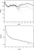 |
Fig. 9 Comparison of column mass densities for two rotation curves that are identical inside solar circle and differ from each other outside the circle. Top panel: original rotation curve as in Figs. 1, 2, (solid line), toy model rotation curve described in the text (dashed line); bottom panel: corresponding column mass densities for a finite-width disk with the Mexican hat vertical profile and height scale of 117 pc. |
With the toy model curve, the results for the vertical gradient of rotation inside the solar circle is not changed significantly in a large region, as shown in Fig. 10, even though the predicted column density at the solar circle is significantly changed, by a factor of 2.
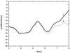 |
Fig. 10 Vertical gradient of rotation at z = 100 kpc for the original rotation curve and for the toy model curve. The gradient prediction is still high and not significantly changed in a region 0−7 kpc, compared with its absolute value. (The local minimum close to 8 kpc is a result of a discontinuity in the toy model curve.) |
This change would also not much influence the results well inside the solar circle for quantities that are integrals over a large region, such as the integrated optical depth we modeled here.
6. Summary and concluding remarks
We obtained the mass distribution in finite-width disks in an iterative fashion from a given rotation curve. We assumed that the volume density ρ(r,z) could be factorized as ρ(r,z) = σ(r)f(z), where f(z) is a normalized vertical profile, with a characteristic width-scale that is a free parameter. We did not assume any constraints on the column mass density σ(r), so that its functional dependence was governed entirely by the shape of the rotation curve. The density effectively describes all forms of the dynamical mass inferred from the Galactic rotation, therefore, the disk-width should not be confused with the width-scale parameters measured in the vicinity of the Sun for various stellar subsystems3.
Based on the gravitational microlensing measurements, it was possible within the disk model framework to determine the effective width-scales. We tested the mass distributions by comparing the model predictions for the vertical gradient of the azimuthal velocity with the gradient measurements.
The (integrated) optical depth from the microlensing measurements is influenced by the amount of mass distributed along the lines of sight towards the Galactic center, whereas the details of the distribution are less important. We inferred the optimum width-scales of the considered disks by means of finding the best fits to the optical depth measured along various lines of sight. This shows that microlensing can be used as a tool to independently constrain the mass distribution models. With these width-scales, the resulting prediction for the behavior of the vertical gradient of rotation was compared with the gradient measurements in the mid-plane vicinity. This comparison is consistent with a small disk thickness. (Interestingly enough, for these width-scales, the effective disk widths defined by the 1/e criterion are almost equal: 2h′ = 176 pc and ~1.49h = 174 pc, respectively, for the exponential and for the Mexican hat vertical profiles).
The behavior of the vertical gradient of the azimuthal velocity and its value, when calculated at low altitudes above the mid-plane, is very sensitive to the width-scale parameter. At a given altitude in the gradient measurements region, the calculated gradient value changes significantly with the width-scale parameter. When the parameter is too high, the absolute gradient value is too low compared with the measurements. Higher absolute gradients at low altitudes above the mid-plane suggest a smaller effective thickness of the Galactic disk. The rotation velocity is another factor that governs the gradient value. In particular, given a disk thickness and the gradient behavior, one could constrain the allowable range for the motion of the standard of rest at the position of the Sun (the width-scale could be increased for higher Ωo). Testing the vertical structure of the mass distribution with the help of the gradient measurements is thus a particularly sensitive tool, and it is therefore important to have high-accuracy measurements of the gradient at low altitudes above the mid-plane.
The column mass density of flattened mass distributions is sensitive to uncertainties in the circular velocity. This sensitivity can be observed in the approximation of infinitely thin disk model (Binney & Tremaine 1987). It is therefore important to have reliable rotation curves when studying flattened galaxies. However, Galactic rotation is relatively well known inside the solar circle, therefore, with better data, we can expect some differences in the column density to occur close to or outside the solar circle. These changes probably do not significantly influence the results for global quantities inside the solar circle, such as the predicted integrated optical depth or vertical gradient inside the solar circle. In particular, as shown in Sect. 5, with a suitably changed external part of the rotation curve, the disk model prediction for the column density at the solar circle of ≈140 M⊙ pc-2 made with the present rotation curve could be reduced to a local value of ≈70 M⊙ pc-2 inferred in the vicinity of the Sun from Jeans modeling (Kuijken & Gilmore 1991; Zhang et al. 2013).
Online material
Appendix A
A.1. Derivation of Eqs. ( 2 ) and ( 3 )
The kernel function J defined in the introduction is singular at an isolated point (ζ = 0,r = R) and is continuous elsewhere. This singularity is integrable in the principal-value sense in Eqs. (2), and (3). Function J is scale-invariant. In particular, J(r,R,ζ) = J(r/R,1,ζ/R), which means that J is effectively dependent only on two variables: r/R and ζ/R. This property allows us to represent J on a plane as in Fig. A.1.
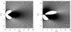 |
Fig. A.1 Contour plots of tanh(J(r,R,ζ)) and
|
Differentiation and taking limits can be interchanged with the integration only under particular conditions imposed on the function under the integration sign. If not said otherwise, we assume that these conditions are met. For this reason, the case of an infinitesimally thin disk (with f(z) = δ(z)) must be treated separately.
The expression for R∂RΨ(R,Z)
in Sect. 2 involves an integral
 The
integral can be written as a sum
The
integral can be written as a sum  if the two summands exist.
By substituting
if the two summands exist.
By substituting  ,
the first integral can be rewritten as
,
the first integral can be rewritten as ![Mathematical equation: \hbox{$\int\limits_{+\infty}^{0} \br{-\ud{\tilde{z}}}\, \rho(r,-\tilde{z})J(r,R,-[\tilde{z}+Z])$}](/articles/aa/full_html/2014/06/aa22919-13/aa22919-13-eq175.png) , and next, since
ρ(r, −
ζ) = ρ(r,ζ) and
J(r,R, −
ζ) = J(r,R,ζ),
as
, and next, since
ρ(r, −
ζ) = ρ(r,ζ) and
J(r,R, −
ζ) = J(r,R,ζ),
as  .
Finally, by renaming
.
Finally, by renaming  , we obtain
This proves Eq. (2).
The integral expression for the vertical gradient of rotation in the quasi-circular
orbit approximation can be proved by performing a partial differentiation of
ℐ under the integration
sign:  Now,
∂ZJ(r,R,z
± Z) = ±
∂zJ(r,R,z
± Z), which implies that
Now,
∂ZJ(r,R,z
± Z) = ±
∂zJ(r,R,z
± Z), which implies that
 .
Integration by parts under usual conditions gives
.
Integration by parts under usual conditions gives
 ,
where ℬ = (limz → +
∞ρ(r,z)[J(r,R,z
+ Z) − J(r,R,z −
Z)]) −
(ρ(r,0+)[J(r,R,Z)
− J(r,R, − Z)]) is
a boundary term. The expression in the first round bracket in this term is zero for any
finite Z,R,r, on account of the vanishing of the
difference in the square bracket and the vanishing of ρ in the same limit (it
suffices to assume a finite support of ρ). The expression in the second round bracket
also vanishes for finite ρ(r,0) since J is an even function of
the third argument. Hence, the boundary term ℬ also vanishes. Formally, one should also verify whether the
integration with respect to r and taking the above limit z → + ∞ commute, as there
is an integration over r present in the expression for R∂RΨ.
When this requirement is met, we have
,
where ℬ = (limz → +
∞ρ(r,z)[J(r,R,z
+ Z) − J(r,R,z −
Z)]) −
(ρ(r,0+)[J(r,R,Z)
− J(r,R, − Z)]) is
a boundary term. The expression in the first round bracket in this term is zero for any
finite Z,R,r, on account of the vanishing of the
difference in the square bracket and the vanishing of ρ in the same limit (it
suffices to assume a finite support of ρ). The expression in the second round bracket
also vanishes for finite ρ(r,0) since J is an even function of
the third argument. Hence, the boundary term ℬ also vanishes. Formally, one should also verify whether the
integration with respect to r and taking the above limit z → + ∞ commute, as there
is an integration over r present in the expression for R∂RΨ.
When this requirement is met, we have  which
proves Eq. (3).
which
proves Eq. (3).
A.2. A special case: the exponential vertical profile
In the case of the vertical exponential falloff of the density profile,
 , the calculation of the
integrals in Eqs. (2) and (3) can be simplified. Then,
, the calculation of the
integrals in Eqs. (2) and (3) can be simplified. Then,
 and
and
 .
Now, both vφ(R,Z)
and ∂Zvφ(R,Z)
can be expressed in terms of two integrals I+ and I−:
.
Now, both vφ(R,Z)
and ∂Zvφ(R,Z)
can be expressed in terms of two integrals I+ and I−:
 Namely,
for ,
Namely,
for ,
 and
and 
A.3. Qualitative properties of the vertical gradient of rotation and the presence of turn-overs
Equation (3) involves an integral
 [ J(r,R,z −
Z)−
J(r,R,z + Z) ]
that equals
[ J(r,R,z −
Z)−
J(r,R,z + Z) ]
that equals  J(r,R,Z −
z), owing to the symmetry of J and f. Now, consider
| Z |
>A>
0 large enough, beyond the main mass concentration, such that
J(r,R,Z −
z), owing to the symmetry of J and f. Now, consider
| Z |
>A>
0 large enough, beyond the main mass concentration, such that
 (by
assumption
(by
assumption  ). For
such Z,
only a region | z | ≪ |
Z | contributes to
). For
such Z,
only a region | z | ≪ |
Z | contributes to
 ,
and we can use the approximation formula J(r,R,Z − z) −
J(r,R,Z) ≈ −z∂ZJ(r,R,Z)
to obtain
,
and we can use the approximation formula J(r,R,Z − z) −
J(r,R,Z) ≈ −z∂ZJ(r,R,Z)
to obtain 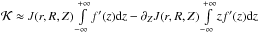 .
Since f(z) and zf(z)
vanish at the infinity, integrating by parts gives
.
Since f(z) and zf(z)
vanish at the infinity, integrating by parts gives
 . On the other hand, for
f(z) =
δ(z) and for Z ≠ 0,
. On the other hand, for
f(z) =
δ(z) and for Z ≠ 0,
 . Hence, we obtain an
intuitively clear result: for all finite-width thin disks with the same column mass
density σ(r), the behavior of the vertical
gradient at high enough altitudes is universal and the same as for an infinitesimally
thin disk with surface mass density σ(r).
. Hence, we obtain an
intuitively clear result: for all finite-width thin disks with the same column mass
density σ(r), the behavior of the vertical
gradient at high enough altitudes is universal and the same as for an infinitesimally
thin disk with surface mass density σ(r).
Another qualitative result is obtained in the limit Z → 0. For
Z ≠ 0,
 ,
thus
,
thus  by continuity of
as a function of Z, and the vertical gradient is zero at
Z = 0, at
least for the mass distributions for which the usual theorems on the continuity of
functions defined by integrals Eq. (3)
apply.
by continuity of
as a function of Z, and the vertical gradient is zero at
Z = 0, at
least for the mass distributions for which the usual theorems on the continuity of
functions defined by integrals Eq. (3)
apply.
However, there is an exception from the above continuity behavior of the gradient lines
at Z = 0.
It is important to remember that the operation of taking various limits and the
operation of integration are not interchangeable in general. In particular, an integral
of a function sequence consisting of continuous functions with a parameter can result in
a discontinuous function of that parameter. For f(z) =
δn(z),
where δn is a functional
sequence representing the Dirac δ, the result of continuity of the gradient does
not necessarily follow and we can have a nonzero value in the same limit, in which case
the integral Eq. (3) is discontinuous at
Z = 0. To
give a simple example of what then may happen, consider a function sequence
 ,
then
,
then  , with
 .
Now, consider a limiting function g(x) = limn → +
∞gn(x)
and see if it is continuous at x = 0. For x = 0, g(0) ≡ limn → +
∞gn(0) = 0, whereas
for x ≠ 0,
.
Now, consider a limiting function g(x) = limn → +
∞gn(x)
and see if it is continuous at x = 0. For x = 0, g(0) ≡ limn → +
∞gn(0) = 0, whereas
for x ≠ 0,
 ,
thus, g(0) = 0 ≠ 1 =
limx → 0g(x),
therefore g(x) is discontinuous at
x = 0.
Now, think of the gradient lines in Fig. 7 – then
the finite disk corresponds to the situation described by gn(x)
(h =
n-1 > 0),
whereas the infinitesimally thin disk corresponds to the situation of discontinuous
g(x) (h = 0).
,
thus, g(0) = 0 ≠ 1 =
limx → 0g(x),
therefore g(x) is discontinuous at
x = 0.
Now, think of the gradient lines in Fig. 7 – then
the finite disk corresponds to the situation described by gn(x)
(h =
n-1 > 0),
whereas the infinitesimally thin disk corresponds to the situation of discontinuous
g(x) (h = 0).
Finally, we may try to understand the occurrence of the turn-overs in the gradient lines for h > 0, such as those seen in Fig. 10 or Fig. 7. First, note that a gradient line must asymptotically converge to zero, which is the universal asymptotics property discussed earlier. Second, the gradient line starts from 0 at Z = 0, which we have also seen above. Now, we perform a mapping of the region 0 < Z < +∞ to an interval 0 < Z < 1 by means of a transformation Z → tanhZ. Then the transformed gradient lines are continuous for 0 ≤ Z ≤ 1 and vanish at the boundaries. Next, we apply the Rolle theorem on continuously differentiable functions that vanish on the boundaries of a compact and simply connected interval, and we infer that there must be at least one point inside the interval where the gradient line has a local minimum, which explains the presence of a turn-over. The Rolle theorem does not apply to gradient lines of the infinitesimally thin disk, because of the discontinuity, and the analogous turn-overs do not have to occur, which is the case in Figs. 7 or 10.
We formulate the criterion as
follows: the effective width-scale h′ of a vertical profile f(z)
integrable to unity is defined by comparing its mass inside a shell | z |
< h′ with that of
an exponential one with a scale-width h′:
 . In
particular, for the Mexican hat profile we obtain
. In
particular, for the Mexican hat profile we obtain  or
2 h′ ≈ 1.49
h.
or
2 h′ ≈ 1.49
h.
The free parameter λ can be used to control the rate of convergence of
the iteration process. We used  instead of 1.
Incidentally, the obtained width-scale of ≈100 pc is consistent with the distribution of massive stars in the vicinity of the Sun. However, massive stars are rare locally and do not contribute substantially to the mass for any proposed IMF.
Acknowledgments
We would like to thank the anonymous referee for a careful reading of our manuscript and for detailed and constructive suggestions that improved the presentation of our results.
References
- Alard, C. 1997, A&A, 321, 424 [NASA ADS] [Google Scholar]
- Alcock, C., Allsman, R. A., Alves, D. R., et al. 2000, ApJ, 542, 281 [NASA ADS] [CrossRef] [Google Scholar]
- Binney, J., & Tremaine, S. 1987, Galactic dynamics (Princeton: Princeton University Press) [Google Scholar]
- Bissantz, N., & Gerhard, O. 2002, MNRAS, 330, 591 [NASA ADS] [CrossRef] [Google Scholar]
- Bissantz, N., Debattista, V. P., & Gerhard, O. 2004, ApJ, 601, L155 [NASA ADS] [CrossRef] [Google Scholar]
- Bovy, J., Hogg, D. W., & Rix, H.-W. 2009, ApJ, 704, 1704 [NASA ADS] [CrossRef] [Google Scholar]
- Bratek, Ł., Jałocha, J., & Kutschera, M. 2008, MNRAS, 391, 1373 [NASA ADS] [CrossRef] [Google Scholar]
- Derue, F., Afonso, C., Alard, C., et al. 2001, A&A, 373, 126 [NASA ADS] [CrossRef] [EDP Sciences] [Google Scholar]
- Gradshtein, I., Ryzhik, I., Jeffrey, A., & Zwillinger, D. 2007, Table of integrals, series and products (Academic Press) [Google Scholar]
- Hamadache, C., Le Guillou, L., Tisserand, P., et al. 2006, A&A, 454, 185 [NASA ADS] [CrossRef] [EDP Sciences] [Google Scholar]
- Jałocha, J., Bratek, Ł., & Kutschera, M. 2008, ApJ, 679, 373 [NASA ADS] [CrossRef] [Google Scholar]
- Jałocha, J., Bratek, Ł., Kutschera, M., & Skindzier, P. 2010, MNRAS, 407, 1689 [NASA ADS] [CrossRef] [Google Scholar]
- Jałocha, J., Bratek, Ł., Kutschera, M., & Skindzier, P. 2011, MNRAS, 412, 331 [NASA ADS] [CrossRef] [Google Scholar]
- Kuijken, K., & Gilmore, G. 1991, ApJ, 367, L9 [NASA ADS] [CrossRef] [Google Scholar]
- Levine, E. S., Heiles, C., & Blitz, L. 2008, ApJ, 679, 1288 [NASA ADS] [CrossRef] [Google Scholar]
- Moniez, M. 2010, Gen. Rel. Grav., 42, 2047 [NASA ADS] [CrossRef] [Google Scholar]
- Paczynski, B. 1986, ApJ, 304, 1 [NASA ADS] [CrossRef] [Google Scholar]
- Popowski, P., Griest, K., Thomas, C. L., et al. (MACHO Collaboration) 2005, ApJ, 631, 879 [NASA ADS] [CrossRef] [Google Scholar]
- Sikora, S., Bratek, Ł., Jałocha, J., & Kutschera, M. 2012, A&A, 546, A126 [NASA ADS] [CrossRef] [EDP Sciences] [Google Scholar]
- Smith, M. C., Woźniak, P., Mao, S., & Sumi, T. 2007, MNRAS, 380, 805 [NASA ADS] [CrossRef] [Google Scholar]
- Sofue, Y., Tutui, Y., Honma, M., et al. 1999, ApJ, 523, 136 [NASA ADS] [CrossRef] [Google Scholar]
- Spitzer, Jr., L. 1942, ApJ, 95, 329 [NASA ADS] [CrossRef] [Google Scholar]
- Sumi, T., Abe, F., Bond, I. A., et al. 2003, ApJ, 591, 204 [NASA ADS] [CrossRef] [Google Scholar]
- Sumi, T., Woźniak, P. R., Udalski, A., et al. 2006, ApJ, 636, 240 [CrossRef] [Google Scholar]
- Wyrzykowski, Ł., Kozłowski, S., Skowron, J., et al. 2011, MNRAS, 413, 493 [NASA ADS] [CrossRef] [Google Scholar]
- Zhang, L., Rix, H.-W., van de Ven, G., et al. 2013, ApJ, 772, 108 [NASA ADS] [CrossRef] [Google Scholar]
All Figures
|
Fig. 1 Column mass densities and the corresponding rotation curves of finite-width disks with a Mexican hat vertical profile (h = 117 pc), shown at several steps of the iteration method of Sect. 2.1, starting from the surface density of an infinitesimally thin disk. Top panel: column mass densities at various iteration steps (thin gray lines), surface mass density of the infinitesimally thin disk model (the starting point of the iteration, triangles), MW column mass density in the final iteration step (it gives the interpolating rotation curve in the bottom panel, solid circles). Bottom panel: (open circles) MW rotation curve points from Sofue et al. (1999), (thin gray lines) rotation curves at various iteration steps, and (thick line) rotation curve in the final iteration step (it strictly overlaps with a spline interpolation of the MW rotation curve points). |
| In the text | |
|
Fig. 2 Optical depth τ(b) in the finite-width disk model for the Mexican hat vertical profile, with the width-scales (1) h = 180 pc; (2) h = 150 pc; (3) h = 117 pc /the best fit/; and (4) h = 100 pc (solid lines). The points with error bars represent the measurement data collected by several collaborations (references in the text). |
| In the text | |
|
Fig. 3 Optical depth τ(b) in the finite-width disk model for the exponential vertical profile with the width-scales (1) h′ = 325 pc; (2) h′ = 200 pc; (3) h′ = 150 pc; (4) h′ = 100 pc; (5) h′ = 88 pc /the best fit/ (solid lines). For comparison, the thick gray line represents the τ(b) in the infinitesimally thin disk model for which the equivalent volume mass density was obtained assuming the exponential vertical profile with h′ = 325 pc. The points with error bars represent measurements data collected by several collaborations (references in the text). |
| In the text | |
|
Fig. 4 Reduced chi-squared, |
| In the text | |
|
Fig. 5 Results of a Monte Carlo simulation: the mean optical depth and its standard deviation for a sample of sources chosen randomly with a probability distribution proportional to ρ(r,z), (points+error bars). For comparison, the (solid line) shows the optical depth calculated with the help of the integral of Eq. (7) with l = 0 and χ = 0. Top panel: results for the Mexican hat vertical profile with h = 117 pc. Bottom panel: results for the exponential vertical profile with h′ = 88 pc. |
| In the text | |
|
Fig. 6 Vertical gradient of rotation in finite-width disk models as a function of altitude above the mid-plane z = 0, shown at various radii: gradient for a disk with the Mexican hat vertical profile (h = 117 pc, solid lines), and gradient for a disk with the exponential vertical profile (h′ = 88 pc, dashed lines). To emphasize the universal gradient behavior at higher altitudes for various disks of the same mass, the results for an infinitesimally thin disk model (with the surface mass density identified with the column mass density of the disk with the Mexican hat vertical profile) is shown (dotted lines). |
| In the text | |
|
Fig. 7 Vertical gradient of rotation in a finite-width disk model with the Mexican hat vertical profile (solid lines), as a function of the altitude above the mid-plane (z = 0), shown at r = 4 kpc for various width-scales h. For comparison, the (dotted line) shows the gradient behavior in the limit of the infinitesimally thin disk model (h → 0). The convergence on that limit is point-wise continuous, although not uniform – the gradient for h = 0 is discontinuous at z = 0. For higher altitudes, the gradient behavior is universal beyond the main concentration of masses. |
| In the text | |
|
Fig. 8 Vertical gradient of rotation of MW in a finite-width disk model with a Mexican hat vertical profile as a function of the radial variable, shown for various width-scales h and altitudes z above the mid-plane. Top panel: gradient at an altitude of 100 pc; – h = 100 pc (dashed line), – h = 117 pc (solid line), and h = 150 pc (uppermost dash-dotted line). (For comparison, the (dash-dotted line) in the middle shows the gradient in a disk model with the vertical exponential profile and the width-scale h′ = 88 pc at the same altitude.) Upper middle panel: vertical gradient of rotation at various altitudes for h = 117 pc. To enable the comparison of structures in the vertical gradient with those in the rotation curve and in the column mass density, Lower middle panel: MW rotation curve, and bottom panel: column mass density for a finite-width disk model with a Mexican hat vertical profile (h = 117 pc). |
| In the text | |
|
Fig. 9 Comparison of column mass densities for two rotation curves that are identical inside solar circle and differ from each other outside the circle. Top panel: original rotation curve as in Figs. 1, 2, (solid line), toy model rotation curve described in the text (dashed line); bottom panel: corresponding column mass densities for a finite-width disk with the Mexican hat vertical profile and height scale of 117 pc. |
| In the text | |
|
Fig. 10 Vertical gradient of rotation at z = 100 kpc for the original rotation curve and for the toy model curve. The gradient prediction is still high and not significantly changed in a region 0−7 kpc, compared with its absolute value. (The local minimum close to 8 kpc is a result of a discontinuity in the toy model curve.) |
| In the text | |
|
Fig. A.1 Contour plots of tanh(J(r,R,ζ)) and
|
| In the text | |
Current usage metrics show cumulative count of Article Views (full-text article views including HTML views, PDF and ePub downloads, according to the available data) and Abstracts Views on Vision4Press platform.
Data correspond to usage on the plateform after 2015. The current usage metrics is available 48-96 hours after online publication and is updated daily on week days.
Initial download of the metrics may take a while.